PH/PH/1 Bulk Arrival and Bulk Service Queue with Randomly Varying Environment

ISSN (e): 2250-3021, ISSN (p): 2278-8719

Vol. 05, Issue 02 (February. 2015), ||V4|| PP 01-12

PH/PH/1 Bulk Arrival and Bulk Service Queue with Randomly

Varying Environment

Ramshankar.R

1

, Rama.G

2

, Sandhya.R

3

, Sundar.V

4

, Ramanarayanan.R

5

1

Independent Researcher MS9EC0, University of Massachusetts, Amherst, MA, USA 2

Independent Researcher B. Tech, Vellore Institute of Technology, Vellore, India 3

Independent Researcher MSPM, School of Business, George Washington University, Washington .D.C, USA 4

Senior Testing Engineer, ANSYS Inc., 2600, Drive, Canonsburg, PA 15317,USA 5

Professor of Mathematics, (Retired), Vel Tech University, Chennai, INDIA.

Abstract: This paper studies two stochastic bulk arrival and bulk service PH/PH/1 queue Models (A) and (B) with randomly varying k* distinct environments. The arrival and service distributions are (𝛼𝑖, 𝑇𝑖) and (𝛽𝑖, 𝑆𝑖) in

the environment i for 1 ≤ i ≤ k* respectively. Whenever the environment changes from i to j the arrival PH and service PH distributions change from the i version to the j version with the exception of the first remaining arrival time and first remaining service time have stationary PH distributions of the j version which is known as equilibrium PH distribution for 1 ≤ i, j ≤ k* and on completion of the same the arrival and service distributions become initial versions (𝛼𝑗, 𝑇𝑗) and (𝛽𝑗, 𝑆𝑗). The queue system has infinite storing capacity and the state space

is identified as five dimensional one to apply Neuts’ matrix methods. The arrivals and the services occur whenever absorptions occur in the corresponding PH distributions. The sizes of the arrivals and the services are finite valued discrete random variables with distinct distributions with respect to environments and with respect to PH phases from which the absorptions occur. Matrix partitioning method is used to study the models. In Model (A) the maximum of the arrival sizes is greater than the maximum of the service sizes and the infinitesimal generator is partitioned mostly as blocks of the sum of the products of PH arrival and PH service phases in the various environments times the maximum of the arrival sizes for analysis. In Model (B) the maximum of the arrival sizes is less than the maximum of the service sizes. The generator is partitioned mostly using blocks of the same sum-product of phases times the maximum of the service sizes. Block circulant matrix structure is noticed in the basic system generators. The stationary queue length probabilities, its expected values, its variances and probabilities of empty levels are derived for the two models using matrix methods.

Numerical examples are presented for illustration.

Keywords: Bulk Arrivals, Bulk Service, Block Circulant Matrix, Neuts Matrix Methods, Phase Type Distribution, Stationary PH Distribution.

I. INTRODUCTION

infinitesimal generator is required to find the stationary probability vector as done in William J. Stewart [11] and matrix geometric structures have not been noted. In such models the recurrence relation method to find the stationary probabilities is stopped at a certain level in most general cases using a terminating analysis very well explained by Qi-Ming He [12] and this stopping limitation of terminating method converts an infinite arrival system to a finite arrival one. In special cases generating function has been identified by Rama and Ramanarayanan [13]. However the division modulo partitioning of the infinitesimal generator along with environment and PH phases used in the paper is presenting matrix geometric solution for finite sized arrivals and services models. The M/PH/1 and PH/M/C queues with random environments have been studied by Usha [14] and [15] without bulk arrivals and bulk services. It has been noticed by Usha [14, 15] that when the environment changes the remaining arrival and service times are to be completed in the new environment. The residual arrival time and the residual service time distributions in the new environment are to be considered in the new environment at an arbitrary epoch since the spent arrival time and the spent service time have been in the previous environment with distinct sizes of PH phase. Further new arrival time and new service time from the start using initial PH distributions of the new environment cannot be considered since the arrival and the service have been partly completed in the previous environment indicating the stationary versions of the arrival and service distributions in the new environments are to be used for the completions of the residual arrival and service times in the new environment and on completion of the same the next arrival and service onwards they have initial versions of the PH distributions of the new environment. The stationary version of the distribution for residual time has been well explained in Qi-Ming He [12] where it is named as equilibrium PH distribution. Randomly varying environment PH/PH/1 queue models with bulk arrival and bulk service have not been treated so far at any depth. In this paper the partitioning of the matrix is carried out in a way that the stationary probability vector exhibits a matrix geometric structure for PH/PH/1 bulk queues with random environment where the arrivals and service sizes are finite. Two models (A) and (B) on PH/PH/1 bulk queue systems with infinite storage space for customers are studied using the block partitioning method. Model (A) presents the case when M, the maximum of the arrival sizes is bigger than N, the maximum of the service sizes. In Model (B), its dual case N is bigger than M, is treated. In general in Queue models, the state space of the system has the first co-ordinate indicating the number of customers in the system but here the customers in the system are grouped and considered as members of blocks of sizes of the maximum for finding the rate matrix. Using the maximum of the bulk arrival size or the maximum of the bulk service size and grouping the customers as members of blocks in addition to coordinates of the arrival and service phases for the partitioning the infinitesimal generator is a new approach in this area. The matrices appearing as the basic system generators in these two models due to block partitioned structure are seen as block circulant matrices. The paper is organized in the following manner. In sections II and III the stationary probability of the number of customers waiting for service, the expectation and the variance and the probability of empty queue are derived for these Models (A) and (B). In section IV numerical cases are presented to illustrate them.

II.MODEL (A): MAXIMUM ARRIVAL SIZE M > MAXIMUM SERVICE SIZE N

2.1Assumptions (i)There are k* environments. The environment changes as per changes in a continuous time Markov chain with

infinitesimal generator 𝑄1 of order k* with stationary probability vector π’.

(ii)In the environment i for 1 ≤ i ≤ k*, the time between consecutive epochs of bulk arrivals of customers has phase type distribution ( 𝛼𝑖, 𝑇𝑖) where 𝑇𝑖is a matrix of order 𝑘𝑖 with absorbing rate 𝑇′𝑖 = −𝑇𝑖𝑒 to the absorbing

state 𝑘𝑖+1 from where the arrival process moves instantaneously to a starting state as per the starting vector 𝛼𝑖

= (𝛼𝑖,1, 𝛼𝑖,2. , …, 𝛼𝑖,𝑘_𝑖) and 𝛼𝑖,𝑗 𝑘𝑖

𝑗 =1 = 1. Let 𝜑𝑖 be the invariant probability vector of the generator matrix

(𝑇𝑖+ 𝑇′𝑖 𝛼𝑖).

(iii) In the environment i for 1 ≤ i ≤ k*,when the absorption occurs in the PH arrival process due to transition from a state j to state 𝑘𝑖+1, 𝑗𝑖𝜒 number of customers arrive with probabilities P (𝑗𝑖𝜒= n) = 𝑗𝑖𝑝𝑛for 1 ≤ n ≤ 𝑗𝑖𝑀

and 𝑗𝑖𝑝𝑛

𝑀

𝑗𝑖

𝑛=1 =1where 𝑗𝑖𝑀 is the maximum arrival size for PH phase j where 1≤ j ≤ 𝑘𝑖 .

(iv) In the environment i for 1 ≤ i ≤ k*, the time between consecutive epochs of bulk services of customers has phase type distribution (𝛽𝑖, 𝑆𝑖) where 𝑆𝑖 is a matrix of order 𝑘′𝑖 with absorbing rate 𝑆′𝑖 = −𝑆𝑖𝑒 to the

absorbing state 𝑘′𝑖+1 from where the service process moves instantaneously to a starting state as per the staring

vector 𝛽𝑖 = (𝛽𝑖,1, 𝛽𝑖,2. , …, 𝛽𝑖,𝑘′_𝑖) and 𝛽𝑖,𝑗 𝑘′_𝑖

𝑗 =1 = 1. Let 𝜙𝑖 be the invariant probability vector of the generator

matrix (𝑆𝑖+ 𝑆′𝑖 𝛽𝑖).

(v) In the environment i for1 ≤ i ≤ k*, customers of bulk size 𝑗𝑖𝜓 are served at epoch when the absorption occurs

due to a transition from state j to state 𝑘′𝑖+1, with probabilities P(𝑗𝑖𝜓 = n) = 𝑗𝑖𝑞𝑛 for 1≤ n ≤ 𝑗𝑖𝑁 and 𝑗𝑖𝑞𝑛 𝑁

𝑗𝑖

𝑗 =1 =

where 1 ≤ j ≤ 𝑘′𝑖 . When n customers n < 𝑗𝑖𝑁 are waiting for service, then n’ customers are served with

probability 𝑗𝑖𝑞𝑛′ for 1≤ n’ ≤ n-1 and n customers are served with probability 𝑗𝑖𝑞𝑛

𝑁

𝑗𝑖

𝑗 =𝑛 for PH phase j where

1 ≤ j ≤ 𝑘′𝑖.

(vi) When the environment changes from i to j for 1 ≤ i, j ≤ k*, the arrival and service distributions in the new environment j are the stationary (equilibrium )versions of arrival time and service time distributions in the new

environment, namely, (𝜑𝑗 , 𝑇𝑗) and (𝜙𝑗, 𝑆𝑗) respectively for the completions of the residual arrival and service

times and on completion of the same the next arrival and service onwards they have initial versions of the PH

distributions of the new environment namely (𝛼𝑗 , 𝑇𝑗) and (𝛽𝑗, 𝑆𝑗) respectively.

(vii) The maximum arrival size M= ma𝑥1≤𝑖≤𝑘 ∗max1 ≤𝑗 ≤𝑘_𝑖𝑗𝑖𝑀 is greater than the maximum service size

N= ma𝑥1≤𝑖≤𝑘 ∗max1 ≤𝑗 ≤𝑘′_𝑖𝑗𝑖𝑁 .

2.2.Analysis

The state of the system of the continuous time Markov chain X (t) under consideration is presented as follows. X(t) = {(0, i, j) : for 1 ≤ i ≤ k* 1 ≤ j ≤ 𝑘𝑖)} U {(0, k, i, j, j’) ; for 1 ≤ k ≤ M-1; 1 ≤ i ≤ k*; 1 ≤ j ≤ 𝑘𝑖; 1 ≤ j ≤ 𝑘′𝑖}

U {(n, k, i, j, j’): for 0 ≤ k ≤ M-1; 1 ≤ i ≤ k*; 1 ≤ j ≤ 𝑘𝑖; 1 ≤ j ≤ 𝑘′𝑖 and n ≥ 1}. (1)

The chain is in the state (0, i, j) when the number of customers in the queue is 0, the environment state is i for 1

≤ i ≤ k*and the arrival phase is j for 1 ≤ j ≤ 𝑘𝑖. The chain is in the state (0, k, i, j, j’) when the number of

customers is k for 1 ≤ k ≤ M-1, the environment state is i for 1 ≤ i ≤ k*, the arrival phase is j for 1 ≤ j ≤ 𝑘𝑖 and

the service phase is j’ for 1 ≤ j’ ≤ 𝑘′𝑖. The chain is in the state (n, k, i, j, j’) when the number of customers in the

queue is n M + k, for 0 ≤ k ≤ M-1 and 1 ≤ n < ∞, the environment state is i for 1 ≤ i ≤ k*, the arrival phase is j

for 1 ≤ j ≤ 𝑘𝑖 and the service phase is j’ for 1 ≤ j’ ≤ 𝑘′𝑖. When the number of customers waiting in the system is

r, then r is identified with (n, k) where r on division by M gives n as the quotient and k as the remainder. Let the survivor probabilities of arrivals𝑗𝑖𝜒 and of services 𝑗𝑖𝜓 be respectively P(𝑗𝑖𝜒>m)= 𝑗𝑖𝑃𝑚=1- 𝑚𝑛=1𝑗𝑖𝑝𝑛,for

1 ≤ m ≤ 𝑗𝑖𝑀-1 and 1≤ j ≤ 𝑘 𝑖 (2)

P(𝑗𝑖𝜓>m)= 𝑗𝑖𝑄𝑚=1- 𝑛=1 𝑚 𝑗𝑖𝑞𝑛, for 1 ≤ m ≤ 𝑗𝑖𝑁-1and 1≤ j ≤ 𝑘′𝑖 (3)

with 𝑗𝑖𝑃0= 1, for all j, 1≤ j ≤ 𝑘𝑖 and 𝑗𝑖𝑄0= 1 for all j , 1≤ j ≤ 𝑘′𝑖 for the environment state i for 1 ≤ i ≤ k* .

The chain X (t) describing model has the infinitesimal generator 𝑄𝐴 of infinite order which can be presented in

block partitioned form given below.

𝑄𝐴=

𝐵1 𝐵0 0 0 . . . ⋯

𝐵2 𝐴1 𝐴0 0 . . . ⋯

0 𝐴2 𝐴1 𝐴0 0 . . ⋯

0 0 𝐴2 𝐴1 𝐴0 0 . ⋯

0 0 0 𝐴2 𝐴1 𝐴0 0 ⋯

⋮ ⋮ ⋮ ⋮ ⋱ ⋱ ⋱ ⋱

(4)

In (4) the states of the matrices are listed lexicographically as 0, 1, 2, 3, …. For partition purpose the zero states

in the first two sets given in (1) are combined. The vector 0 is of type 1 x [ 𝑘∗𝑖=1𝑘𝑖+ (𝑀 − 1) 𝑘∗𝑖=1𝑘𝑖𝑘′𝑖] and is

0=((0,1,1),(0,1,2),(0,1,3)…(0,1, 𝑘1),(0,2,1),(0,2,2),(0,2,3)…(0,2, 𝑘2),……(0,k*,1),(0,k*,2),(0,k*,3)…(0,k*,𝑘𝑘∗),

(0,1,1,1,1),(0,1,1,1,2)….(0,1,1,1, 𝑘′1),(0,1,1,2,1),(0,1,1,2,2)….(0,1,1,2,𝑘′1),(0,1,1,3,1)....(0,1,1,3,𝑘′1)…..(0,1,1,

𝑘1,1)…(0,1,1,𝑘1, 𝑘′1),(0,1,2,1,1),(0,1,2,1,2)….(0,1,2,1, 𝑘′2),(0,1,2,2,1),(0,1,2,2,2)….(0,1,2,2,𝑘′2),(0,1,2,3,1)....(0

,1,2,3,𝑘′2)….(0,1,2,𝑘2,1)…(0,1,2,𝑘2, 𝑘′2),(0,1,3,1,1)…(0,1,3,𝑘3, 𝑘′3)…(0,1,k*,1,1),…,(0,1,k*,𝑘𝑘∗, 𝑘′𝑘∗),(0,2,1,1

,1),(0,2,1,1,2),…,(0,2,k*,𝑘𝑘 ∗,𝑘′𝑘∗),(0,3,1,1,1)…(0,3,k*,𝑘𝑘∗𝑘𝑘 ∗),(0,4,1,1,1)…(0,4,k*,𝑘𝑘 ∗𝑘′𝑘∗)…(0,M-1,1,1,1)…

(0,M-1,k*,𝑘𝑘 ∗, 𝑘′𝑘∗)) and the vector 𝑛 is of type 1x[𝑀 𝑘∗𝑖=1𝑘𝑖𝑘′𝑖] and is given in a similar manner as follows

𝑛=(n,0,1,1,1),(n,0,1,1,2)….(n,0,1,1, 𝑘′1),(n,0,1,2,1),…(n,0,1,2,𝑘′1),…(n,0,k*,1,1),…(n,0,k*,𝑘𝑘 ∗, 𝑘′𝑘∗),(n,1,1,1,1)

….(n,1,k*,𝑘𝑘∗,𝑘′𝑘 ∗),(n,2,1,1,1)....(n,2,k*,𝑘𝑘 ∗,𝑘′𝑘∗)……..(n,M-1,1,1,1),(n,M-1,1,1,2)……(n,M-1,k*,𝑘𝑘∗, 𝑘′𝑘∗)).

The matrices𝐵1𝑎𝑛𝑑 𝐴1 have negative diagonal elements, they are of orders [ 𝑘∗𝑖=1𝑘𝑖+ (𝑀 − 1) 𝑘∗𝑖=1𝑘𝑖𝑘′𝑖] and

[𝑀 𝑘∗𝑖=1𝑘𝑖𝑘′𝑖] respectively and their off diagonal are non-negative.

The matrices 𝐴0 𝑎𝑛𝑑𝐴2 have nonnegative elements and are of order [ 𝑀 𝑘∗𝑖=1𝑘𝑖𝑘′𝑖 ] . The matrices 𝐵0 𝑎𝑛𝑑 𝐵2

have non-negative elements and are of types [ 𝑘∗𝑖=1𝑘𝑖+ (𝑀 − 1) 𝑘∗𝑖=1𝑘𝑖𝑘′𝑖] x [ 𝑀 𝑘∗𝑖=1𝑘𝑖𝑘′𝑖 ] and

[ 𝑀 𝑘∗𝑖=1𝑘𝑖𝑘′𝑖 ] x [ 𝑘∗𝑖=1𝑘𝑖+ (𝑀 − 1) 𝑘∗𝑖=1𝑘𝑖𝑘′𝑖]. Component matrices of 𝐴𝑖 𝑎𝑛𝑑 𝐵𝑖for i=0,1,2 are defined

below. Let ⊕ 𝑎𝑛𝑑 ⨂ denote the Kronecker sum and Kronecker product.

Let 𝒬𝑖′=𝑇𝑖⊕ 𝑆𝑖 + diag ((𝑄1)𝑖,𝑖) = (𝑇𝑖⨂𝐼𝑘′𝑖) + ( 𝐼𝑘𝑖⨂𝑆𝑖) + diag ((𝑄1)𝑖,𝑖) for 1 ≤ i ≤ k* (5)

where I indicates the identity matrices of orders given in the suffixes, 𝒬𝑖′ is of order 𝑘𝑖𝑘′𝑖 and the last term is a

diagonal matrix of order 𝑘𝑖𝑘′𝑖 . Considering the change of environment switches on stationary distributions in

PH arrival time and PH service time in the new environment, the following matrix Ω of order 𝑘∗𝑖=1𝑘𝑖𝑘′𝑖is

Ω=

𝚀′1 𝛺1,2 𝛺1,3 ⋯ 𝛺1,𝑘∗

𝛺2,1 𝚀′2 𝛺2,3 ⋯ 𝛺2,𝑘∗

𝛺3,1 𝛺3,2 𝚀′3 ⋯ 𝛺3,𝑘∗

⋮ ⋮ ⋮ ⋱ ⋮

𝛺𝑘∗,1 𝛺𝑘∗,2 𝛺𝑘∗,3 ⋯ 𝚀′𝑘∗

(6)

where 𝛺𝑖,𝑗 is a rectangular matrix of type 𝑘𝑖𝑘′𝑖 x 𝑘𝑗𝑘′𝑗whose all rows are equal to (𝑄1)𝑖,𝑗 (𝜑𝑗 ⨂𝜙𝑗) for i ≠ j ,

1 ≤ i, j ≤ k*. The arrival rate of n customers for 1≤ n ≤ 𝑗𝑖𝑀 corresponding to absorption to state 𝑘𝑖+1 from the

arrival PH phase j for 1≤ j ≤ 𝑘𝑖, in the environment i for 1≤ i ≤ k* is given by the component j of the column

vector 𝑇_𝑖,𝑛′

of type 𝑘𝑖 x1 where 𝑇𝑖,𝑛′ = ( (𝑇′𝑖)1(1𝑖𝑝𝑛) , (𝑇′𝑖)2(2𝑖𝑝𝑛) , (𝑇′𝑖)3(3𝑖𝑝𝑛) , ….(𝑇′𝑖)𝑘_𝑖(𝑘𝑖𝑝𝑛 𝑖

) )’; (7)

the service rate of n customers for 1≤ n ≤ _𝑗𝑖𝑁

corresponding to absorption to state 𝑘′𝑖+1 from the service PH

phase j for 1≤ j ≤ 𝑘′𝑖, in the environment i for 1≤ i ≤ k* is given by the component j of the column vector 𝑆𝑖,𝑛′

of type 𝑘′𝑖 x1where 𝑆𝑖,𝑛′ = ( (𝑆′𝑖)1(1𝑖𝑞𝑛) , (𝑆′𝑖)2(2𝑖𝑞𝑛) , (𝑆′𝑖)3(3𝑖𝑞𝑛) , ….(𝑆′𝑖)𝑘′𝑖(𝑘′𝑖𝑞𝑛

𝑖 _{))’ . (8)}

Let 𝛬𝑛 =

𝑇1,𝑛′ 𝛼1⊗ 𝐼𝑘′₁ 0 0 ⋯ 0

0 𝑇2,𝑛′ 𝛼2⊗ 𝐼𝑘′2 0 ⋯ 0

0 0 𝑇3,𝑛′ 𝛼3⊗ 𝐼𝑘′3 ⋯ 0

⋮ ⋮ ⋮ ⋱ ⋮

0 0 0 ⋯ 𝑇𝑘 ∗,𝑛′ 𝛼𝑘∗⊗ 𝐼𝑘′_𝑘∗

for 1 ≤ n ≤ M (9)

In (9) 𝛬𝑛 is a square matrix of order 𝑘∗𝑖=1𝑘𝑖𝑘′𝑖; 𝑇𝑗 ,𝑛′ 𝛼𝑗⊗ 𝐼𝑘′_𝑗is a square matrix of order 𝑘𝑗𝑘′𝑗 for 1 ≤ j ≤ k* and

0 appearing as (i, j) component of (9) is a block zero rectangular matrix of type 𝑘𝑖𝑘′𝑖 x 𝑘𝑗𝑘′𝑗 .

Let 𝑈𝑛 =

𝐼𝑘1⊗ 𝑆1,𝑛

′ _𝛽

1 0 0 ⋯ 0

0 𝐼𝑘2⊗ 𝑆2,𝑛

′ _𝛽

2 0 ⋯ 0

0 0 𝐼𝑘3⊗ 𝑆3,𝑛

′ _𝛽

3 ⋯ 0

⋮ ⋮ ⋮ ⋱ ⋮

0 0 0 ⋯ 𝐼𝑘_𝑘∗⊗ 𝑆𝑘 ∗,𝑛′ 𝛽𝑘∗

for 1 ≤ n ≤ N (10)

In (10) 𝑈𝑛 is a square matrix of order 𝑘∗𝑖=1𝑘𝑖𝑘′𝑖; 𝐼𝑘_𝑗 ⊗ 𝑆𝑗 ,𝑛′ 𝛽𝑗is a square matrix of order 𝑘𝑗𝑘′𝑗 for 1 ≤ j ≤ k*

and 0 appearing as (i, j) component of (10) is a block zero rectangular matrix of type 𝑘𝑖𝑘′𝑖 x 𝑘𝑗𝑘′𝑗 .The matrix 𝐴𝑖

for i = 0,1,2are as follows.

𝐴0=

𝛬𝑀 0 ⋯ 0 0 0

𝛬𝑀−1 𝛬𝑀 ⋯ 0 0 0

𝛬𝑀−2 𝛬𝑀−1 ⋯ 0 0 0

𝛬𝑀−3 𝛬𝑀−2 ⋱ 0 0 0

⋮ ⋮ ⋱ ⋱ ⋮ ⋮

𝛬3 𝛬4 ⋯ 𝛬𝑀 0 0

𝛬2 𝛬3 ⋯ 𝛬𝑀−1 𝛬𝑀 0

𝛬1 𝛬2 ⋯ 𝛬𝑀−2 𝛬𝑀−1 𝛬𝑀

(11) 𝐴2 =

0 ⋯ 0 𝑈𝑁 𝑈𝑁−1 ⋯ 𝑈2 𝑈1

0 ⋯ 0 0 𝑈𝑁 ⋯ 𝑈3 𝑈2

⋮ ⋮ ⋮ ⋮ ⋮ ⋱ ⋮ ⋮

0 ⋯ 0 0 0 ⋯ 𝑈𝑁 𝑈𝑁−1

0 ⋯ 0 0 0 ⋯ 0 𝑈𝑁

0 ⋯ 0 0 0 ⋯ 0 0

⋮ ⋮ ⋮ ⋮ ⋮ ⋮ ⋮ ⋮

0 ⋯ 0 0 0 ⋯ 0 0

(12)

𝐴1=

𝛺 𝛬1 𝛬2 ⋯ 𝛬𝑀−𝑁−2 𝛬𝑀−𝑁−1 𝛬𝑀−𝑁 ⋯ 𝛬𝑀−2 𝛬𝑀−1

𝑈1 𝛺 𝛬1 ⋯ 𝛬𝑀−𝑁−3 𝛬𝑀−𝑁−2 𝛬𝑀−𝑁−1 ⋯ 𝛬𝑀−3 𝛬𝑀−2

𝑈2 𝑈1 𝛺 ⋯ 𝛬𝑀−𝑁−4 𝛬𝑀−𝑁−3 𝛬𝑀−𝑁−2 ⋯ 𝛬𝑀−4 𝛬𝑀−3

⋮ ⋮ ⋮ ⋱ ⋮ ⋮ ⋮ ⋱ ⋮ ⋮

𝑈𝑁 𝑈𝑁−1 𝑈𝑁−2 ⋯ 𝛺 𝛬1 𝛬2 ⋯ 𝛬𝑀−𝑁−2 𝛬𝑀−𝑁−1

0 𝑈𝑁 𝑈𝑁−1 ⋯ 𝑈1 𝛺 𝛬1 ⋯ 𝛬𝑀−𝑁−3 𝛬𝑀−𝑁−2

0 0 𝑈𝑁 ⋯ 𝑈2 𝑈1 𝛺 ⋯ 𝛬𝑀−𝑁−4 𝛬𝑀−𝑁−3

⋮ ⋮ ⋮ ⋱ ⋮ ⋮ ⋮ ⋱ ⋮ ⋮

0 0 0 ⋯ 𝑈𝑁 𝑈𝑁−1 𝑈𝑁−2 ⋯ 𝛺 𝛬1

0 0 0 ⋯ 0 𝑈𝑁 𝑈𝑁−1 ⋯ 𝑈1 𝛺

(13)

For defining the matrices 𝐵𝑖 for i = 0,1,2 the following component matrices are required

𝛬′𝑛 =

𝑇1,𝑛′ 𝛼1⊗ 𝛽1 0 0 ⋯ 0

0 𝑇2,𝑛′ 𝛼2⊗ 𝛽2 0 ⋯ 0

0 0 𝑇3,𝑛′ 𝛼3⊗ 𝛽3 ⋯ 0

⋮ ⋮ ⋮ ⋱ ⋮

0 0 0 ⋯ 𝑇𝑘 ∗,𝑛′ 𝛼𝑘∗⊗ 𝛽𝑘 ∗

for 1 ≤ n ≤ M (14)

𝛬′𝑛 is a rectangular matrix of type ( 𝑖=1𝑘∗ 𝑘𝑖)x k∗i=1(𝑘𝑖𝑘′𝑖) for 1 ≤ n ≤ M ; 𝑇𝑖,𝑛′ 𝛼𝑖⊗ 𝛽𝑖 is a rectangular matrix

for 1 ≤ i, j ≤ k*. Let 𝑉′𝑖,𝑛= 𝐼𝑘_𝑖⊗ ( (𝑆′𝑖)1( 𝑄1𝑖 𝑛) , (𝑆′𝑖)2( 𝑄2𝑖 𝑛) , (𝑆′𝑖)3( 𝑄3𝑖 𝑛) , … . (𝑆′𝑖)𝑘′𝑖 𝑘′_𝑖𝑄𝑛

𝑖 _)′

for 1 ≤ n ≤ N -1 is a matrix of type 𝑘𝑖𝑘′𝑖 x 𝑘𝑖 for 1 ≤ i ≤ k*and let

𝑉𝑛 =

𝑉′1,𝑛 0 0 ⋯ 0

0 𝑉′2,𝑛 0 ⋯ 0

⋮ ⋮ ⋮ ⋱ ⋮

0 0 0 ⋯ 𝑉′𝑘∗,𝑛

for 1 ≤ n ≤ N. (15)

This is a rectangular matrix of type ( 𝑖=𝑘 ∗𝑖=1 𝑘𝑖𝑘′𝑖) 𝑥 𝑘∗𝑖=1𝑘𝑖 and 0 appearing in the (i, j) component is a

rectangular 0 matrix of type 𝑘𝑖𝑘′𝑖 x 𝑘𝑗 for 1 ≤ i, j ≤ k*.

Let U =

𝐼𝑘1⊗ 𝑆1

′ _{0 0 ⋯ 0}

0 𝐼𝑘₂⊗ 𝑆2′ 0 ⋯ 0

⋮ ⋮ ⋮ ⋱ ⋮

0 0 0 ⋯ 𝐼𝑘₁⊗ 𝑆𝑘 ∗′

(16)

In (16), U is a rectangular matrix of type ( 𝑖=𝑘∗𝑖=1 𝑘𝑖𝑘′𝑖) 𝑥 𝑘∗𝑖=1𝑘𝑖 and 0 appearing in the (i, j) component is a

rectangular 0 matrix of type 𝑘𝑖𝑘′𝑖 x 𝑘𝑗 for 1 ≤ i, j ≤ k*. 𝐼𝑘𝑖 ⨂𝑆𝑖

′ _{is a rectangular matrix of type 𝑘}

𝑖𝑘′𝑖 𝑥 𝑘𝑖 for 1 ≤

i ≤ k*. The matrix 𝐵0 is same as that of 𝐴0 when 𝛬𝑀 in the first row of 𝐴0is replaced by𝛬′𝑀. The matrix 𝐵1 is

given below. The matrix 𝐵2 is same as that of 𝐴2when the first block column with 0 is considered as 𝑘∗𝑖=1𝑘𝑖

columns block instead of 𝑘∗𝑖=1𝑘𝑖𝑘′𝑖columns block of 𝐴2. To write 𝐵1the block for 0 is to be considered which

has queue length, L= 0, 1, 2…M-1. When L = 0 there is only arrival process and no service process. The change in environment from i to j switches on stationary PH (equilibrium PH) distribution in the new environment j whenever it occurs for 1 ≤ i ≠ j, ≤ k*. When an arrival occurs and queue length becomes L in the environment i

both the arrival time and the service time start with starting probability vector 𝛼𝑖 and 𝛽𝑖 respectively for 1 ≤ i ≤

k*. In the 0 when L =1,2, …M-1 all the processes arrival, service and environment are active as in other blocks

𝑛 for n > 0. Considering the change of environment switches on the stationary (equilibrium) distribution in PH

arrival time in the new environment when the queue is empty, the following matrix Ω’ of order 𝑘∗𝑖=1𝑘𝑖is defined

which is concerned with change of environment during arrival time.

Ω’=

𝑇′1 𝛺′1,2 𝛺′1,3 ⋯ 𝛺′1,𝑘∗

𝛺′2,1 𝑇′2 𝛺′2,3 ⋯ 𝛺′2,𝑘∗

𝛺′3,1 𝛺′3,2 𝑇′3 ⋯ 𝛺′3,𝑘∗

⋮ ⋮ ⋮ ⋱ ⋮

𝛺′𝑘∗,1 𝛺′𝑘∗,2 𝛺′𝑘∗,3 ⋯ 𝑇′𝑘∗

(17)

Here 𝑇′𝑖= 𝑇𝑖+ 𝑑𝑖𝑎𝑔(𝑄1)𝑖,𝑖 and 𝛺′𝑖,𝑗 is a rectangular matrix of type 𝑘𝑖 x 𝑘𝑗whose all rows are equal to

(𝑄1)𝑖,𝑗 𝜑𝑗 presenting the rates of changing to phases in the new environment for i ≠ j and 1 ≤ i, j ≤ k*.

𝐵1=

𝛺′ 𝛬′1 𝛬′2 ⋯ 𝛬′𝑀−𝑁−2 𝛬′𝑀−𝑁−1 𝛬′𝑀−𝑁 ⋯ 𝛬′𝑀−2 𝛬′𝑀−1

𝑈 𝛺 𝛬1 ⋯ 𝛬𝑀−𝑁−3 𝛬𝑀−𝑁−2 𝛬𝑀−𝑁−1 ⋯ 𝛬𝑀−3 𝛬𝑀−2

𝑉1 𝑈1 𝛺 ⋯ 𝛬𝑀−𝑁−4 𝛬𝑀−𝑁−3 𝛬𝑀−𝑁−2 ⋯ 𝛬𝑀−4 𝛬𝑀−3

⋮ ⋮ ⋮ ⋱ ⋮ ⋮ ⋮ ⋱ ⋮ ⋮

𝑉𝑁−1 𝑈𝑁−1 𝑈𝑁−2 ⋯ 𝛺 𝛬1 𝛬2 ⋯ 𝛬𝑀−𝑁−2 𝛬𝑀−𝑁−1

0 𝑈𝑁 𝑈𝑁−1 ⋯ 𝑈1 𝛺 𝛬1 ⋯ 𝛬𝑀−𝑁−3 𝛬𝑀−𝑁−2

0 0 𝑈𝑁 ⋯ 𝑈2 𝑈1 𝛺 ⋯ 𝛬𝑀−𝑁−4 𝛬𝑀−𝑁−3

⋮ ⋮ ⋮ ⋱ ⋮ ⋮ ⋮ ⋱ ⋮ ⋮

0 0 0 ⋯ 𝑈𝑁 𝑈𝑁−1 𝑈𝑁−2 ⋯ 𝛺 𝛬1

0 0 0 ⋯ 0 𝑈𝑁 𝑈𝑁−1 ⋯ 𝑈1 𝛺

(18)

𝒬_𝐴′ ₌

𝛺 + 𝛬𝑀 𝛬1 ⋯ 𝛬𝑀−𝑁−2 𝛬𝑀−𝑁−1 𝛬𝑀−𝑁+ 𝑈𝑁 ⋯ 𝛬𝑀−2+ 𝑈2 𝛬𝑀−1+ 𝑈1

𝛬𝑀−1+ 𝑈1 𝛺 + 𝛬𝑀 ⋯ 𝛬𝑀−𝑁−3 𝛬𝑀−𝑁−2 𝛬𝑀−𝑁−1 ⋯ 𝛬𝑀−3+ 𝑈3 𝛬𝑀−2+ 𝑈2

𝛬𝑀−2+ 𝑈2 𝛬𝑀−1+ 𝑈1 ⋯ 𝛬𝑀−𝑁−4 𝛬𝑀−𝑁−3 𝛬𝑀−𝑁−2 ⋯ 𝛬𝑀−4+ 𝑈3 𝛬𝑀−3+ 𝑈3

⋮ ⋮ ⋮⋮⋮ ⋮ ⋮ ⋮ ⋮⋮⋮ ⋮ ⋮

𝛬𝑀−𝑁+2+ 𝑈𝑁−2 . ⋯ . . . ⋯ 𝛬𝑀−𝑁+ 𝑈𝑁 𝛬𝑀−𝑁+1+ 𝑈𝑁−1

𝛬𝑀−𝑁+1+ 𝑈𝑁−1 . ⋯ . . . . 𝛬𝑀−𝑁−1 𝛬𝑀−𝑁+ 𝑈𝑁

𝛬𝑀−𝑁+ 𝑈𝑁 . ⋯ 𝛺 + 𝛬𝑀 𝛬1 𝛬2 ⋯ 𝛬𝑀−𝑁−2 𝛬𝑀−𝑁−1

𝛬𝑀−𝑁−1 𝛬𝑀−𝑁+ 𝑈𝑁 ⋯ 𝛬𝑀−1+ 𝑈1 𝛺 + 𝛬𝑀 𝛬1 ⋯ 𝛬𝑀−𝑁−3 𝛬𝑀−𝑁−2

𝛬𝑀−𝑁−2 𝛬𝑀−𝑁−1 ⋯ 𝛬𝑀−2+ 𝑈2 𝛬𝑀−1+ 𝑈1 𝛺 + 𝛬𝑀 ⋯ 𝛬𝑀−𝑁−4 𝛬𝑀−𝑁−3

⋮ ⋮ ⋮⋮⋮ ⋮ ⋮ ⋮ ⋮⋮⋮ ⋮ ⋮

𝛬2 𝛬3 ⋯ 𝛬𝑀−𝑁+ 𝑈𝑁 𝛬𝑀−𝑁+1+ 𝑈𝑁−1 𝛬𝑀−𝑁+2+ 𝑈𝑁−2 ⋯ 𝛺 + 𝛬𝑀 𝛬1

𝛬1 𝛬2 ⋯ 𝛬𝑀−𝑁−1 𝛬𝑀−𝑁+ 𝑈𝑁 𝛬𝑀−𝑁+1+ 𝑈𝑁−1 ⋯ 𝛬𝑀−1+ 𝑈1 𝛺 + 𝛬𝑀

(19)

The basic generator of the bulk queue which is concerned with only the arrival and service is a matrix of order

Its probability vector w’ gives, 𝑤′𝒬_𝐴′ =0 and w’. e = 1 (21)

It is well known that a square matrix in which each row (after the first) has the elements of the previous row

shifted cyclically one place right, is called a circulant matrix. It is very interesting to note that the matrix 𝒬𝐴′ is

a block circulant matrix where each block matrix is rotated one block to the right relative to the preceding block

partition. In (19), the first block-row of type [ 𝑘∗𝑖=1𝑘𝑖𝑘′𝑖 ] x[ 𝑀 𝑖=1𝑘∗ 𝑘𝑖𝑘′𝑖 ] is, 𝑊 = (𝛺 + 𝛬𝑀, 𝛬1, 𝛬2 ,

…, 𝛬𝑀−𝑁−2, 𝛬𝑀−𝑁−1, 𝛬𝑀−𝑁+ 𝑈𝑁, …, 𝛬𝑀−2+ 𝑈2, 𝛬𝑀−1+ 𝑈1) which gives as the sum of the blocks 𝛺 +

𝛬𝑀 + 𝛬1+ 𝛬2 +…+𝛬𝑀−𝑁−2+ 𝛬𝑀−𝑁−1+ 𝛬𝑀−𝑁+ 𝑈𝑁+…+𝛬𝑀−2+ 𝑈2+ 𝛬𝑀−1+ 𝑈1= Ω’’ which is the matrix

given by

Ω’’=

𝚀′′1 𝛺1,2 𝛺1,3 ⋯ 𝛺1,𝑘∗

𝛺2,1 𝚀′′2 𝛺2,3 ⋯ 𝛺2,𝑘∗

𝛺3,1 𝛺3,2 𝚀′′3 ⋯ 𝛺3,𝑘∗

⋮ ⋮ ⋮ ⋱ ⋮

𝛺𝑘∗,1 𝛺𝑘∗,2 𝛺𝑘∗,3 ⋯ 𝚀′′𝑘∗

(22)

where using (5) and (6), 𝑄’’𝑖 = ((𝑇𝑖+ 𝑇′𝑖 𝛼𝑖)⨂𝐼𝑘′𝑖) + ( 𝐼𝑘𝑖⨂(𝑆𝑖+ 𝑆′𝑖 𝛽𝑖)) + diag ((𝑄1)𝑖,𝑖) for 1 ≤ i ≤ k*. The stationary probability vector of the basic generator given in (19) is required to get the stability condition. Consider the vector w = ( 𝜋′1𝜑1⊗ 𝜙1, 𝜋′2𝜑2⊗ 𝜙2,…, 𝜋′𝑘∗𝜑𝑘 ∗⊗ 𝜙𝑘∗) where π’ = (𝜋′1, 𝜋′2, … , 𝜋′𝑘∗) is the

stationary probability vector of the environment, 𝜑𝑖 𝑎𝑛𝑑 𝜙𝑖 are the stationary probability vectors of the arrival

and service PH processes (𝑇𝑖 + 𝑇′𝑖 𝛼𝑖) and (𝑆𝑖+ 𝑆′𝑖 𝛽𝑖) respectively. It may be noted 𝜋′𝑖(𝜑𝑖⊗ 𝜙𝑖)[((𝑇𝑖+

𝑇′𝑖 𝛼𝑖)⨂𝐼𝑘′

𝑖) + ( 𝐼𝑘𝑖⨂(𝑆𝑖+ 𝑆

′

𝑖 𝛽𝑖))] =0. This gives 𝜋′𝑖(𝜑𝑖⊗ 𝜙𝑖)𝑄’’𝑖 = 𝜋′𝑖(𝑄1)𝑖,𝑖 (𝜑𝑖⊗ 𝜙𝑖) 𝐼 = 𝜋′𝑖(𝑄1)𝑖,𝑖

(𝜑𝑖 ⊗ 𝜙𝑖) for 1 ≤ i ≤ k*. Now the first column of the matrix multiplication of wΩ’’ is 𝜋′1(𝑄1)1,1𝜑1,1𝜙1,1 +

𝜋′2 (𝑄1)2,1𝜑11𝜙11[(𝜑2⊗ 𝜙2)𝑒] +...+ 𝜋′𝑘∗ (𝑄1)𝑘 ∗,1𝜑11𝜙11[(𝜑𝑘 ∗⊗ 𝜙𝑘∗)]𝑒 = 0 since (𝜑𝑖⊗ 𝜙𝑖)𝑒 = 1 and

π′𝑄1=0. In a similar manner it can be seen that the first column block of wΩ’’ is 𝜋′1(𝑄1)1,1𝜑1⊗ 𝜙1 +

𝜋′2 (𝑄1)2,1𝜑1⊗ 𝜙1[(𝜑2⊗ 𝜙2)𝑒] +...+ 𝜋′𝑘∗ (𝑄1)𝑘 ∗,1𝜑1⊗ 𝜙1[(𝜑𝑘∗⊗ 𝜙𝑘∗)]𝑒 = 0 and i-th column block is

𝜋′1(𝑄1)1,𝑖𝜑𝑖⊗ 𝜙𝑖[(𝜑1⊗ 𝜙1)𝑒] +𝜋′2 (𝑄1)2,𝑖𝜑𝑖⊗ 𝜙𝑖[(𝜑2⊗ 𝜙2)𝑒] +...+𝜋′𝑖 (𝑄1)𝑖,𝑖𝜑𝑖⊗ 𝜙𝑖+…+

𝜋′𝑘∗ (𝑄1)𝑘 ∗,𝑖𝜑𝑖⊗ 𝜙𝑖[(𝜑𝑘∗⊗ 𝜙𝑘∗)]𝑒= 0. This shows that 𝑤 𝛺 + 𝛬𝑀 + 𝑤𝛬1+ 𝑤𝛬2 +…+𝑤𝛬𝑀−𝑁−2+

𝑤𝛬𝑀−𝑁−1+ 𝑤𝛬𝑀−𝑁+ 𝑤𝑈𝑁+…+𝑤𝛬𝑀−2+ 𝑤𝑈2+ 𝑤𝛬𝑀−1+ 𝑤𝑈1= w Ω’’=0. So (w, w,…,w) .W= 0 = (w, w,

….w) W’ where W’ is the transpose W. This shows (w,w...w) is the left eigen vector of 𝒬_𝐴′ _{and the}

corresponding probability vector is w’ = 𝑤

𝑀, 𝑤 𝑀, 𝑤 𝑀, … . . , 𝑤

𝑀 where w is given by

w = ( 𝜋′1(𝜑1⊗ 𝜙1), 𝜋′2(𝜑2⊗ 𝜙2),……, 𝜋′𝑘∗(𝜑𝑘 ∗⊗ 𝜙𝑘∗) ) (23)

Let 𝜑𝑖 = (𝜑𝑖 ,𝑗) and 𝜙𝑖 = (𝜙𝑖 ,𝑗) be the stationary probability components of the arrival and service processes.

Neuts [5], gives the stability condition as, w′ 𝐴0 𝑒 < 𝑤′ 𝐴2 𝑒 where w is given by (23). Taking the sum

cross diagonally in the 𝐴0 𝑎𝑛𝑑 𝐴2 matrices, it can be seen using (9) that

w’ 𝐴0 𝑒= 1

𝑀 𝑤 𝑛𝛬𝑛

𝑀

𝑛=1 𝑒=

1

𝑀 𝑛

𝑘∗

𝑖=1 𝜋′𝑖(𝜑𝑖⊗ 𝜙𝑖)(𝑇𝑖,𝑛′ ⊗ 𝑒) 𝑀

𝑛=1 =

1

𝑀 𝑛

𝑘∗

𝑖=1 𝜋′𝑖(𝜑𝑖𝑇𝑖,𝑛′ ⊗ 𝜙𝑖𝑒)

𝑀

𝑛=1 =

1

𝑀 𝑛

𝑘∗

𝑖=1 𝜋′𝑖(𝜑𝑖𝑇𝑖,𝑛′ )

𝑀 𝑛=1 = 1 𝑀( 𝜋′𝑖 𝑛 𝑀 𝑛=1 𝑘∗

𝑖=1 𝜑𝑖,𝑗

𝑘_𝑖

𝑗 =1 (𝑇𝑖,𝑛′ )𝑗)

=1

𝑀( 𝜋′𝑖 𝑛

𝑀 𝑛=1 𝑘∗

𝑖=1 𝜑𝑖,𝑗

𝑘_𝑖

𝑗 =1 (𝑇′𝑖)𝑗 𝑝𝑗𝑖 𝑛 ) =

1

𝑀( 𝜋′𝑖 𝜑𝑖,𝑗(

𝑘_𝑖 𝑗 =1 𝑘∗

𝑖=1 𝑇′𝑖)𝑗E(𝑗𝑖𝜒)<𝑤′𝐴2 𝑒

=1

𝑀 𝑤 𝑛𝑈𝑛

𝑁

𝑛=1 𝑒=

1

𝑀 𝑛

𝑘∗

𝑖=1 𝜋′𝑖(𝜑𝑖⊗ 𝜙𝑖)(𝑒 ⊗ 𝑆𝑖,𝑛′ ) 𝑁

𝑛=1 =

1

𝑀 𝑛

𝑘∗

𝑖=1 𝜋′𝑖(𝜑𝑖𝑒 ⊗ 𝜙𝑖𝑆𝑖,𝑛′ ) 𝑁

𝑛=1

=_𝑀1 𝑘∗ 𝑛

𝑖=1 𝜋′𝑖(𝜙𝑖𝑆𝑖,𝑛′ )

𝑁 𝑛=1 = 1 𝑀( 𝜋′𝑖 𝑛 𝑁 𝑛=1 𝑘∗

𝑖=1 𝜙𝑖,𝑗

𝑘′_𝑖

𝑗 =1 (𝑆𝑖,𝑛′ )𝑗)

=1

𝑀( 𝜋′𝑖 𝑛

𝑁 𝑛=1 𝑘∗

𝑖=1 𝜙𝑖,𝑗

𝑘′𝑖

𝑗 =1 (𝑆′𝑖)𝑗 𝑞𝑗𝑖 𝑛 )=

1

𝑀( 𝜋′𝑖 𝜙𝑖,𝑗(

𝑘′𝑖

𝑗 =1 𝑘∗

𝑖=1 𝑆′𝑖)𝑗E(𝑗𝑖𝜓). This gives the stability condition

as 𝜋′𝑖 𝜑𝑖,𝑗(

𝑘𝑖

𝑗 =1 𝑘∗

𝑖=1 𝑇′𝑖)𝑗E(𝑗𝑖𝜒) < 𝜋′𝑖 𝜙𝑖,𝑗(

𝑘′𝑖

𝑗 =1 𝑘∗

𝑖=1 𝑆′𝑖)𝑗E(𝑗𝑖𝜓) (24)

From the result (24) result for the case of PH/PH/1 bulk queue without environment Ramshankar et al., [8] can

be deduced. This result (24) is the stability condition for the random environment PH/PH/1 bulk queue with

random sizes of arrivals and of services where maximum arrival size is greater than the maximum service size.

When (24) is satisfied, the stationary distribution of the queue length exists Neuts [5]. Let π(0, i, j) : for 1 ≤ i ≤

k* 1 ≤ j ≤ 𝑘𝑖; π(0, k, i, j, j’) ; for 1 ≤ k ≤ M-1; 1 ≤ i ≤ k*; 1 ≤ j ≤ 𝑘𝑖; 1 ≤ j ≤ 𝑘′𝑖 and π(n, k, i, j, j’): for 0 ≤ k ≤

M-1; 1 ≤ i ≤ k*; 1 ≤ j ≤ 𝑘𝑖; 1 ≤ j ≤ 𝑘′𝑖 and n ≥ 1 be the stationary probability vectors of Markov chain X(t) states.

Let 𝜋0=

(

π(0,1,1),π(0,1,2),…π(0,1,𝑘1),π(0,2,1),π(0,2,2),……π(0,2,𝑘2),……,π(0,k*,1),π(0,k*,2),……π(0,k*,𝑘𝑘 ∗),

π(0,1,1,1,1),π(0,1,1,1,2)…π(0,1,1,𝑘1, 𝑘′1),π(0,1,2,1,1),π(0,1,2,1,2)…π(0,1,2,𝑘2, 𝑘′2),π(0,1,3,1,1),π(0,1,3,1,2)…

π(0,1,3,𝑘2, 𝑘′2)…π(0,1,k*,1,1),π(0,1,k*,1,2)……π(0,1,k*,𝑘𝑘 ∗, 𝑘′𝑘∗),π(0,2,1,1,1),……π(0,2,k*,𝑘𝑘∗ , 𝑘′𝑘∗)………

π(0,M-1,1,1,1),π(0,M-1,1,1,2)……π(0,M-1,k*,𝑘𝑘 ∗ , 𝑘′𝑘∗)

)

be a vector of type 1x[ 𝑖=1𝑘∗ 𝑘𝑖+ (𝑀 − 1) 𝑘∗𝑖=1𝑘𝑖𝑘′𝑖].

Let 𝜋𝑛=

(

π(n,0,1,1,1),π(n,0,1,1,2)……π(n,0,1,𝑘1, 𝑘′1),π(n,0,2,1,1),π(n,0,2,1,2)……π(n,0,2,𝑘2, 𝑘′2),π(n,0,3,1,1),

π(n,0,3,1,2)…π(n,0,3,𝑘3, 𝑘′3)…π(n,0,k*,1,1),π(n,0,k*,1,2)……π(n,0,k*,𝑘𝑘∗, 𝑘′𝑘 ∗),π(n,1,1,1,1),π(n,1,1,1,2)……

π(n,1,1,𝑘1, 𝑘′1),π(n,1,2,1,1),π(n,1,2,1,2)……π(n,1,2,𝑘2, 𝑘′2),π(n,1,3,1,1),π(n,1,3,1,2)……π(n,1,3,𝑘3, 𝑘′3)……

π(n,3,k*,𝑘𝑘 ∗, 𝑘′𝑘 ∗)….π(n,M-1,1,1,1),π(n,M-1,1,1,2)………π(n,M-1,k*,𝑘𝑘 ∗ , 𝑘′𝑘∗)

)

be a vector of type

1x[𝑀 𝑘∗𝑖=1𝑘𝑖𝑘′𝑖]. The stationary probability vector 𝜋 = (𝜋0, 𝜋1, 𝜋3, … ) satisfies the equations

𝜋𝑄𝐴=0 and πe=1. (25)

From (25), it can be seen 𝜋0𝐵1+ 𝜋1𝐵2=0. (26)

𝜋0𝐵0+𝜋1𝐴1+𝜋2𝐴2 = 0 (27)

𝜋𝑛−1𝐴0+𝜋𝑛𝐴1+𝜋𝑛+1𝐴2 = 0, for n ≥ 2. (28)

Introducing the rate matrix R as the minimal non-negative solution of the non-linear matrix equation

𝐴0+R𝐴1+𝑅2𝐴2=0, (29)

it can be proved (Neuts [5]) that 𝜋𝑛 satisfies the following. 𝜋𝑛 = 𝜋1 𝑅𝑛−1 for n ≥ 2. (30)

Using (26), 𝜋0 satisfies 𝜋0 = 𝜋1𝐵2(−𝐵1)−1 (31)

So using (27) and (31) and (30) the vector 𝜋1 can be calculated up to multiplicative constant since 𝜋1 satisfies

the equation 𝜋1 [𝐵2 −𝐵1 −1𝐵0+ 𝐴1+ 𝑅𝐴2] =0. (32)

Using (31) and (30) it can be seen that 𝜋1[𝐵2(−𝐵1)−1e+(I-R)−1𝑒] = 1. (33)

Replacing the first column of the matrix multiplier of 𝜋1 in equation (32), by the column vector multiplier of

𝜋1 in (33), a matrix which is invertible may be obtained. The first row of the inverse of that same matrix is 𝜋1

and this gives along with (31) and (30) all the stationary probabilities of the system. The matrix R is iterated starting with 𝑅 0 = 0; and finding 𝑅(𝑛 + 1)=−𝐴0𝐴1−1–𝑅2(𝑛)𝐴2𝐴1−1, for n ≥ 0. The iteration may be

terminated to get a solution of R at a norm level where 𝑅 𝑛 + 1 − 𝑅(𝑛 ) < ε.

2.3. Performance Measures of the System

(i) The probability of the queue length S = r > 0, P(S=r) can be seen as follows. For 1 ≤ r ≤ M-1, P(S =r) = 𝜋(0, 𝑟, 𝑖, 𝑗1, 𝑗2

𝑘′1

𝑗2=1

𝑘𝑖

𝑗1=1

𝑘∗

𝑖=1 ). For r ≥ M, let n and k be non negative integers such that r = n M + k. Then

P(S=r) = 𝜋(𝑛, 𝑘, 𝑖, 𝑗1, 𝑗2

𝑘′_𝑖 𝑗2=1

𝑘_𝑖 𝑗1=1

𝑘∗

𝑖=1 ) , where r = n M + k, n ≥ 1 and k ≥ 0. (34)

(ii) The probability that the queue length is zero is P(S =0) = 𝑘𝑖 𝜋 0, 𝑖, 𝑗 .

𝑗 =1 𝑘∗

𝑖=1 (35)

(iii) The expected queue level E(S), can be calculated. Using (35) and (34), it may be seen that

E(S)= 𝑟∞

0 𝑃(𝑆 = 𝑟)= 0𝜋 0, 𝑖, 𝑗 𝑘_𝑖

𝑗 =1 𝑘∗

𝑖=1 + 𝑘𝜋(0, 𝑘, 𝑖, 𝑗1, 𝑗2

𝑘′_𝑖 𝑗₂=1 𝑘_𝑖

𝑗₁=1 𝑘∗

𝑖=1 )

𝑀−1 𝑘=1

+ 𝜋(𝑛, 𝑘, 𝑖, 𝑗1, 𝑗2

𝑘′_𝑖 𝑗2=1

𝑘_𝑖 𝑗1=1

𝑘∗

𝑖=1 )(𝑛𝑀 + 𝑘)

𝑀−1 𝑘 =0

∞

𝑛=1

= 𝑘𝜋(0, 𝑘, 𝑖, 𝑗1, 𝑗2

𝑘′𝑖

𝑗2=1

𝑘𝑖

𝑗1=1

𝑘∗

𝑖=1 ) +

𝑀−1

𝑘 =1 ∞𝑛=1𝜋𝑛.(Mn,…,Mn,Mn+1,…,Mn+1,Mn+2,…,Mn+2,…,

Mn+M-1,…,Mn+M-1) = 𝑘 𝜋(0, 𝑘, 𝑖, 𝑗1, 𝑗2

𝑘′_𝑖 𝑗2=1

𝑘_𝑖 𝑗1=1

𝑘∗

𝑖=1 ) +

𝑀−1

𝑘=1 M ∞𝑛=1𝑛𝜋𝑛𝑒+𝜋1( 𝐼 − 𝑅)−1𝜉.

Here ξ= 0, … 0,1, … ,1,2, … ,2, … , 𝑀 − 1, … , 𝑀 − 1 ′ is of type [( 𝑘∗𝑖=1𝑘𝑖𝑘′𝑖)M]x1 column vector

in which consecutively ( 𝑘∗𝑖=1𝑘𝑖𝑘′𝑖) times 0,1,2,3.., M-1 appear. Let it be called ξ’ when 0 appears

( 𝑘∗𝑖=1𝑘𝑖)times and others in that order appear ( 𝑘∗𝑖=1𝑘𝑖𝑘′𝑖) times.

Then E(S)= 𝜋0ξ’+ 𝜋1( 𝐼 − 𝑅)−1𝜉 + 𝑀𝜋1(𝐼 − 𝑅 )−2𝑒 (36)

(iv)Variance of S can be derived. Let η be column vector η=[0, . . ,0, 12_{, … 1}2 ₂2_{, . . , 2}2_{, … 𝑀 − 1)}2_{, … , (𝑀 −}

1)2′ of type [(𝑖=1𝑘∗𝑘𝑖𝑘′𝑖)M]x1in which consecutively (𝑖=1𝑘∗𝑘𝑖𝑘′𝑖) times squares of 0,1,2,3.., M-1 appear. Let

it be called η’ when 0 appears ( 𝑘∗𝑖=1𝑘𝑖) times and others in the same manner as in η appear ( 𝑘∗𝑖=1𝑘𝑖𝑘′𝑖) times.

Then it can be seen that the second moment, E(𝑆2_{)= 𝑟}∞ 2

0 𝑃(𝑆 = 𝑟)= 0𝜋 0, 𝑖, 𝑗

𝑘_𝑖 𝑗 =1 𝑘∗

𝑖=1 + 𝜋(0, 𝑘, 𝑖, 𝑗1, 𝑗2

𝑘′_𝑖 𝑗2=1

𝑘_𝑖 𝑗1=1

𝑘∗

𝑖=1 )𝑘2

𝑀−1 𝑘=1

+ 𝜋(𝑛, 𝑘, 𝑖, 𝑗1, 𝑗2

𝑘′𝑖

𝑗2=1

𝑘𝑖

𝑗1=1

𝑘∗

𝑖=1 )(𝑛𝑀 + 𝑘)2

𝑀−1 𝑘 =0

∞

𝑛=1 =𝜋0η’+ 𝑀2 𝑛=1∞ 𝑛 𝑛 − 1 𝜋𝑛𝑒 + ∞𝑛=1𝑛𝜋𝑛𝑒 +

𝜋𝑛𝜂

∞

𝑛=1 + 2M ∞𝑛=1𝑛 𝜋𝑛𝜉.

So, E(𝑆2_{)= 𝜋}

0η’+𝑀2[𝜋1(𝐼 − 𝑅)−32𝑅 𝑒 + 𝜋1(𝐼 − 𝑅)−2𝑒] + 𝜋1(𝐼 − 𝑅)−1𝜂 + 2𝑀𝜋1(𝐼 − 𝑅)−2𝜉 (37)

VAR(S)=E(𝑆2_{) − [𝐸(𝑆)]}2_{may be written from (36) and(37).}

III. MODEL (B) MAXIMUM ARRIVAL SIZE M < MAXIMUM SERVICE SIZE N The dual case of Model (A), namely the case, M < N is treated here. (When M =N both models are

applicable and one can use any one of them.) The assumption (vii) of Model (A) is changed and all its other

assumptions are retained.

3.1

.

Assumption

(vii) The maximum arrival size M= ma𝑥1≤𝑖≤𝑘 ∗max1 ≤𝑗 ≤𝑘𝑖𝑗𝑀

𝑖 _{is less than the maximum service size}

N=ma𝑥1≤𝑖≤𝑘∗max1 ≤𝑗 ≤𝑘′𝑖𝑗𝑁

3.2

.

Analysis

Since this model is dual, the analysis is similar to that of Model (A). The differences are noted below. The state space of the chain is as follows presented in a similar way.

The state of the system of the continuous time Markov chain X (t) under consideration is presented as follows. X(t) = {(0, i, j) : for 1 ≤ i ≤ k* 1 ≤ j ≤ 𝑘𝑖)} U {(0, k, i, j, j’) ; for 1 ≤ k ≤ N-1; 1 ≤ i ≤ k*; 1 ≤ j ≤ 𝑘𝑖; 1 ≤ j ≤ 𝑘′𝑖}

U {(n, k, i, j, j’): for 0 ≤ k ≤ N-1; 1 ≤ i ≤ k*; 1 ≤ j ≤ 𝑘𝑖; 1 ≤ j ≤ 𝑘′𝑖 and n ≥ 1}. (38)

The chain is in the state (0, i, j) when the number of customers in the queue is 0, the environment state is i for 1 ≤ i ≤ k*and the arrival phase is j for 1 ≤ j ≤ 𝑘𝑖. The chain is in the state (0, k, i, j, j’) when the number of

customers is k for 1 ≤ k ≤ N-1, the environment state is i for 1 ≤ i ≤ k*, the arrival phase is j for 1 ≤ j ≤ 𝑘𝑖 and

the service phase is j’ for 1 ≤ j’ ≤ 𝑘′𝑖. The chain is in the state (n, k, i, j, j’) when the number of customers in the

queue is n N + k, for 0 ≤ k ≤ N-1 and 1 ≤ n < ∞, the environment state is i for 1 ≤ i ≤ k*, the arrival phase is j for

1 ≤ j ≤ 𝑘𝑖 and the service phase is j’ for 1 ≤ j’ ≤ 𝑘′𝑖. When the number of customers waiting in the system is r,

then r is identified with (n, k) where r on division by N gives n as the quotient and k as the remainder. The

infinitesimal generator 𝑄𝐵 of the model has the same structure given in (4) but the inner matrices are of different

orders.

𝑄𝐵=

𝐵′

1 𝐵′0 0 0 . . . ⋯

𝐵′

2 𝐴′1 𝐴′0 0 . . . ⋯

0 𝐴′

2 𝐴′1 𝐴′0 0 . . ⋯

0 0 𝐴′

2 𝐴′1 𝐴′0 0 . ⋯

0 0 0 𝐴′

2 𝐴′1 𝐴′0 0 ⋯

⋮ ⋮ ⋮ ⋮ ⋱ ⋱ ⋱ ⋱

(39)

In (39) the states of the matrices are listed lexicographically as 0, 1, 2, 3, …. For partition purpose the zero states

in the first two sets of (38) are combined. The vector 0 is of type 1 x [ 𝑘∗𝑖=1𝑘𝑖+ (𝑁 − 1) 𝑘∗𝑖=1𝑘𝑖𝑘′𝑖] and is

0=((0,1,1),(0,1,2),…(0,1, 𝑘1),(0,2,1),(0,2,2),…(0,2, 𝑘2),……(0,k*,1),(0,k*,2),…(0,k*,𝑘𝑘∗),(0,1,1,1,1),(0,1,1,1,2)

….(0,1,1,1, 𝑘′1),(0,1,1,2,1),(0,1,1,2,2)….(0,1,1,2,𝑘′1),(0,1,1,3,1)....(0,1,1,3,𝑘′1)…..(0,1,1,𝑘1,1)…

(0,1,1,𝑘1, 𝑘′1),(0,1,2,1,1),(0,1,2,1,2)….(0,1,2,1, 𝑘′2),(0,1,2,2,1),(0,1,2,2,2)….(0,1,2,2,𝑘′2),(0,1,2,3,1)....(0,1,2,3,

𝑘′2)….(0,1,2,𝑘2,1)…(0,1,2,𝑘2, 𝑘′2),(0,1,3,1,1)…(0,1,3,𝑘3, 𝑘′3)…(0,1,k*,1,1),….(0,1,k*,𝑘𝑘∗, 𝑘′𝑘∗),(0,2,1,1,1),

(0,2,1,1,2)…(0,2,k*,𝑘𝑘∗,𝑘′𝑘 ∗),(0,3,1,1,1)…(0,3,k*,𝑘𝑘 ∗𝑘𝑘∗),(0,4,1,1,1)…(0,4,k*,𝑘𝑘 ∗𝑘′𝑘∗)…(0,N-1,1,1,1)…

(0,N-1,k*,𝑘𝑘 ∗, 𝑘′𝑘∗)) and the vector 𝑛 is of type 1x[𝑁 𝑘∗𝑖=1𝑘𝑖𝑘′𝑖] and is given in a similar manner as follows

𝑛=(n,0,1,1,1),(n,0,1,1,2)….(n,0,1,1, 𝑘′1),(n,0,1,2,1),…(n,0,1,2,𝑘′1),…(n,0,k*,1,1),…(n,0,k*,𝑘𝑘 ∗, 𝑘′𝑘∗),(n,1,1,1,1)

…. (n,1,k*,𝑘𝑘∗,𝑘′𝑘∗),(n,2,1,1,1)....(n,2,k*,𝑘𝑘∗,𝑘′𝑘 ∗)……..(n,N-1,1,1,1),(n,N-1,1,1,2)……(n,N-1,k*,𝑘𝑘 ∗, 𝑘′𝑘∗)).

The matrices𝐵′1𝑎𝑛𝑑 𝐴′1 have negative diagonal elements, they are of orders [ 𝑘∗𝑖=1𝑘𝑖+ (𝑁 − 1) 𝑘∗𝑖=1𝑘𝑖𝑘′𝑖] and

[𝑁 𝑘∗𝑖=1𝑘𝑖𝑘′𝑖] respectively and their off diagonal elements are non-negative.

The matrices 𝐴′0 𝑎𝑛𝑑𝐴′2 have nonnegative elements and are of order [ 𝑁 𝑘∗𝑖=1𝑘𝑖𝑘′𝑖 ] . The matrices

𝐵′0 𝑎𝑛𝑑 𝐵′2 have non-negative elements and are of types [ 𝑘∗𝑖=1𝑘𝑖+ (𝑁 − 1) 𝑖=1𝑘∗ 𝑘𝑖𝑘′𝑖] x [ 𝑁 𝑘∗𝑖=1𝑘𝑖𝑘′𝑖 ]

and [ 𝑁 𝑘∗𝑖=1𝑘𝑖𝑘′𝑖 ] x [ 𝑖=1𝑘∗ 𝑘𝑖+ (𝑁 − 1) 𝑘∗𝑖=1𝑘𝑖𝑘′𝑖] and they are given below. Using Model (A) for

definitions of 𝛬𝑗 𝑎𝑛𝑑𝛬′𝑗, 𝑎𝑛𝑑 𝑈𝑗, 𝑉𝑗, and U and lettingΩ and Ω’ as in Model (A), the partitioning matrices are

defined as follows. The matrix 𝐵′0is same as that of 𝐴′0 with first zero block row is of order[ 𝑘∗𝑖=1𝑘𝑖] x[

𝑁 𝑘 ∗𝑖=1𝑘𝑖𝑘′𝑖]. The matrix 𝐵′2is same as that of 𝐴′2 except the first column block is of type [ 𝑁 𝑘∗𝑖=1𝑘𝑖𝑘′𝑖 ] x

[ 𝑘∗𝑖=1𝑘𝑖] and is (𝑈′𝑁, 0, … .0)′ where

𝑈′𝑁=

𝐼𝑘1⊗ 𝑆1,𝑁

′ _{0 0 ⋯ 0}

0 𝐼𝑘2⊗ 𝑆2,𝑁

′ _{0 ⋯ 0}

0 0 𝐼𝑘3⊗ 𝑆3,𝑁

′ _{⋯ 0}

⋮ ⋮ ⋮ ⋱ ⋮

0 0 0 ⋯ 𝐼𝑘_𝑘∗⊗ 𝑆𝑘 ∗,𝑁′

(40)

𝐴′0=

0 0 ⋯ 0 0 0 ⋯ 0

⋮ ⋮ ⋯ ⋮ ⋮ ⋮ ⋮ ⋮

0 0 ⋯ 0 0 0 ⋯ 0

𝛬𝑀 0 ⋯ 0 0 0 ⋯ 0

𝛬𝑀−1 𝛬𝑀 ⋯ 0 0 0 ⋯ 0

⋮ ⋮ ⋱ ⋮ ⋮ ⋮ ⋮ ⋮

𝛬2 𝛬3 ⋯ 𝛬𝑀 0 0 ⋯ 0

𝛬1 𝛬2 ⋯ 𝛬𝑀−1 𝛬𝑀 0 ⋯ 0

𝐴′2=

𝑈𝑁 𝑈𝑁−1 𝑈𝑁−2 ⋯ 𝑈3 𝑈2 𝑈1

0 𝑈𝑁 𝑈𝑁−1 ⋯ 𝑈4 𝑈3 𝑈2

0 0 𝑈𝑁 ⋯ 𝑈5 𝑈4 𝑈3

0 0 0 ⋱ 𝑈6 𝑈5 𝑈4

⋮ ⋮ ⋮ ⋱ ⋮ ⋮ ⋮

0 0 0 ⋯ 𝑈𝑁 𝑈𝑁−1 𝑈𝑁−2

0 0 0 ⋯ 0 𝑈𝑁 𝑈𝑁−1

0 0 0 ⋯ 0 0 𝑈𝑁

(42)

𝐴′1=

Ω 𝛬1 𝛬2 ⋯ 𝛬𝑀 0 0 ⋯ 0 0

𝑈1 Ω 𝛬1 ⋯ 𝛬𝑀−1 𝛬𝑀 0 ⋯ 0 0

𝑈2 𝑈1 Ω ⋯ 𝛬𝑀−2 𝛬𝑀−1 𝛬𝑀 ⋯ 0 0

⋮ ⋮ ⋮ ⋱ ⋮ ⋮ ⋮ ⋱ ⋮ ⋮

𝑈𝑁−𝑀−1 𝑈𝑁−𝑀−2 𝑈𝑁−𝑀−3 ⋯ Ω 𝛬1 𝛬2 ⋯ 𝛬𝑀−1 𝛬𝑀

𝑈𝑁−𝑀 𝑈𝑁−𝑀−1 𝑈𝑁−𝑀−2 ⋯ 𝑈1 Ω 𝛬1 ⋯ 𝛬𝑀−2 𝛬𝑀−1

𝑈𝑁−𝑀+1 𝑈𝑁−𝑀 𝑈𝑁−𝑀−1 ⋯ 𝑈2 𝑈1 Ω ⋯ 𝛬𝑀−3 𝛬𝑀−2

⋮ ⋮ ⋮ ⋱ ⋮ ⋮ ⋮ ⋱ ⋮ ⋮

𝑈𝑁−2 𝑈𝑁−3 𝑈𝑁−4 ⋯ 𝑈𝑁−𝑀−2 𝑈𝑁−𝑀−3 𝑈𝑁−𝑀−2 ⋯ Ω 𝛬1

𝑈𝑁−1 𝑈𝑁−2 𝑈𝑁−3 ⋯ 𝑈𝑁−𝑀−1 𝑈𝑁−𝑀−2 𝑈𝑁−𝑀−1 ⋯ 𝑈1 Ω

(43)

𝐵′1=

𝛺′ 𝛬′1 𝛬′2 ⋯ 𝛬′𝑀 0 0 ⋯ 0 0

𝑈 Ω 𝛬1 ⋯ 𝛬𝑀−1 𝛬𝑀 0 ⋯ 0 0

𝑉1 𝑈1 Ω ⋯ 𝛬𝑀−2 𝛬𝑀−1 𝛬𝑀 ⋯ 0 0

⋮ ⋮ ⋮ ⋱ ⋮ ⋮ ⋮ ⋱ ⋮ ⋮

𝑉𝑁−𝑀−2 𝑈𝑁−𝑀−2 𝑈𝑁−𝑀−3 ⋯ Ω 𝛬1 𝛬2 ⋯ 𝛬𝑀−1 𝛬𝑀

𝑉𝑁−𝑀−1 𝑈𝑁−𝑀−1 𝑈𝑁−𝑀−2 ⋯ 𝑈1 Ω 𝛬1 ⋯ 𝛬𝑀−2 𝛬𝑀−1

𝑉𝑁−𝑀 𝑈𝑁−𝑀 𝑈𝑁−𝑀−1 ⋯ 𝑈2 𝑈1 Ω ⋯ 𝛬𝑀−3 𝛬𝑀−2

⋮ ⋮ ⋮ ⋱ ⋮ ⋮ ⋮ ⋱ ⋮ ⋮

𝑉𝑁−3 𝑈𝑁−3 𝑈𝑁−4 ⋯ 𝑈𝑁−𝑀−2 𝑈𝑁−𝑀−3 𝑈𝑁−𝑀−2 ⋯ Ω 𝛬1

𝑉𝑁−2 𝑈𝑁−2 𝑈𝑁−3 ⋯ 𝑈𝑁−𝑀−1 𝑈𝑁−𝑀−2 𝑈𝑁−𝑀−1 ⋯ 𝑈1 Ω

(44)

𝒬_𝐵′′ ₌

𝛺 + 𝑈𝑁 𝛬1+ 𝑈𝑁−1 ⋯ 𝛬𝑀−1+ 𝑈𝑁−𝑀+1 𝛬𝑀+ 𝑈𝑁−𝑀 𝑈𝑁−𝑀−1 ⋯ 𝑈2 𝑈1

𝑈1 𝛺 + 𝑈𝑁 ⋯ 𝛬𝑀−2+ 𝑈𝑁−𝑀+2` 𝛬𝑀−1+ 𝑈𝑁−𝑀+1 𝛬𝑀+ 𝑈𝑁−𝑀 ⋯ 𝑈3 𝑈2

⋮ ⋮ ⋮⋮⋮ ⋮ ⋮ ⋮ ⋮⋮⋮ ⋮ ⋮

𝑈𝑁−𝑀−2 𝑈𝑁−𝑀−3 ⋯ 𝛺 + 𝑈𝑁 𝛬1+ 𝑈𝑁−1 𝛬2+ 𝑈𝑁−2 ⋯ 𝛬𝑀+ 𝑈𝑁−𝑀 𝑈𝑁−𝑀−1

𝑈𝑁−𝑀−1 𝑈𝑁−𝑀−2 ⋯ 𝑈1 𝛺 + 𝑈𝑁 𝛬1+ 𝑈𝑁−1 ⋯ 𝛬𝑀−1+ 𝑈𝑁−𝑀+1 𝛬𝑀+ 𝑈𝑁−𝑀

𝛬𝑀+ 𝑈𝑁−𝑀 𝑈𝑁−𝑀−1 ⋯ 𝑈2 𝑈1 𝛺 + 𝑈𝑁 ⋯ 𝛬𝑀−2+ 𝑈𝑁−𝑀+2 𝛬𝑀−1+ 𝑈𝑁−𝑀+1

⋮ ⋮ ⋮⋮⋮ ⋮ ⋮ ⋮ ⋮⋮⋮ ⋮ ⋮

𝛬2+ 𝑈𝑁−2 𝛬3+ 𝑈𝑁−3 ⋯ 𝑈𝑁−𝑀−1 𝑈𝑁−𝑀−2 𝑈𝑁−𝑀−3 ⋯ 𝛺 + 𝑈𝑁 𝛬1+ 𝑈𝑁−1

𝛬1+ 𝑈𝑁−1 𝛬2+ 𝑈𝑁−2 ⋯ 𝛬𝑀+ 𝑈𝑁−𝑀 𝑈𝑁−𝑀−1 𝑈𝑁−𝑀−2 ⋯ 𝑈1 𝛺 + 𝑈𝑁

(45)

The basic generator which is concerned with only the arrival and service is 𝒬𝐵′′ = 𝐴′0+ 𝐴′1+ 𝐴′2. This is also

block circulant. Using similar arguments given for Model (A) it can be seen that its probability vector is w’ =

𝑤

𝑁,

𝑤

𝑁,

𝑤 𝑁, … . . ,

𝑤

𝑁 where w is given by w = ( 𝜋′1(𝜑1⊗ 𝜙1), 𝜋′2(𝜑2⊗ 𝜙2),……, 𝜋′𝑘∗(𝜑𝑘∗⊗ 𝜙𝑘∗) ) and the

stability condition remains the same. Following the arguments given for Model (A), one can find the stationary probability vector for Model (B) also in matrix geometric form. All performance measures including expectation of customers waiting for service and its variance for Model (B) have the form as in Model (A) except M is replaced by N.

IV. NUMERICAL ILLUSTRATIONS

Numerical cases are presented here to illustrate the application of the study. Three examples are studied namely (i) M=N=3 (ii) M=3, N=2 and (iii) M=2, N=3. The environment has two states governed by the Markov chain

with infinitesimal generator −3 3

5 −5 . In state 1, the arrival time distribution is PH 1 (exponential) with

parameter 5 and the service time distribution is PH 2with representation −3 1

2 −3 and starting probability

vector (.6, .4). In environment 2 the arrival time has PH 2 distribution with representation −2 1

2 −4 and

starting probability vector (.4, .6) and the service time distribution is PH 1 (exponential) with parameter 8. For the case (i) M=N=3, in the environment 1, the probabilities of bulk arrivals are taken as 11𝑝1=.6, 11𝑝2=.2 and

𝑝3 1 1

=.2 and the probabilities of bulk services in the two phases are considered as 11𝑞=.5, 11𝑞2=.3, 11𝑞3=.2, 21𝑞1=.4,

𝑞2 2 1

=.6 and 21𝑞3=0. In the environment 2, the bulk arrival probabilities are assumed as 12𝑝1=.4, 12𝑝2=.6, 12𝑝3=0,

𝑝1 2

2 _{=.5, 𝑝}

2 2

2 _{=.5 and 𝑝}

3 2

2 _{=0 and bulk service probabilities are taken as 𝑞}

1 2

2 _{=.5, 𝑞}

2 2

2 _{=.5 and 𝑞}

3 2

2 _{=0. For the case (ii)}

values of case (i) for all others. For the case (iii) M=2, N=3, the probabilities of case (i) are assumed changing

only two values namely, 11𝑝2=.4 and 11𝑝3= 0. The rate matrix R is taken for calculation after 30 iterations for the

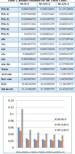
three models. The results obtained are presented in the table 1 below. The probabilities and expected values show significant variation for higher and lower values of M and N. The figures (1) and (2) show the variations of probabilities.

Table 1. Results Obtained for the Three Cases.

M=N=3 M=3;N=2 M=2;N=3

P(S=0) 0.060354629 0.050226694 0.115130656 P(S=1) 0.027940388 0.02353663 0.053013985 P(S=2) 0.026006538 0.022495782 0.04491614 P(S=3) 0.025331264 0.022031479 0.042021471 P(S=4) 0.024460863 0.021384356 0.039162694 P(S=5) 0.0236716 0.020802411 0.036546073 π0e 0.116536161 0.097720416 0.227289746 π1e 0.081693776 0.070317631 0.144526435 π2e 0.073463727 0.064218246 0.117730239 π3e 0.06669037 0.059222531 0.095641597 π4e 0.060580626 0.054651446 0.077721784 π(n>4)e 0.601035341 0.653869731 0.337090199

Norm 0.000630675 0.000681993 0.00032906 Arri rate 1.694444444 1.694444444 1.518518519 Serv rate 2.462962963 2.433333333 2.462962963 E(S) 29.86540309 36.01090259 13.28458975 Std dev(S) 31.21206209 37.35092795 14.41652322

Figure 1. Probabilities of Queue Lengths 0

0.02 0.04 0.06 0.08 0.1 0.12 0.14

P(S=0)P(S=1)P(S=2)P(S=3)P(S=4)P(S=5) M=N=3

M=3;N=2

Figure2.The Probabilities of Customer Blocks

V. CONCLUSION

Two PH/PH/1 bulk arrival and bulk service queues with random environment have been studied by identifying the maximum of the arrival and service sizes and grouping the customers as members of blocks of such maximum sizes. Matrix geometric results have been obtained by partitioning the infinitesimal generator by grouping of customers, environment state and PH phases together. The basic system generators of the queues are block circulant matrices which are explicitly presenting the stability condition in standard forms. Numerical results for bulk queue models are presented and discussed. Effects of variation of rates on expected queue length and on probabilities of queue lengths are exhibited. The decrease in arrival rates (so also increase in service rates) makes the convergence of R matrix faster which can be seen in the decrease of norm values. The standard deviations also decrease. The PH/PH/1 queue with bulk arrival and bulk service with random environment has number of applications. The PH distributions include Exponential, Erlang, Hyper Exponential, and Coxian distributions as special cases and the PH distribution is also a best approximation for a general distribution. Further the PH/PH/1 queue is a most general form almost equivalent to G/G/1 queue. The bulk arrival models because they have non zero elements or blocks above the super diagonals in infinitesimal generators, they require for studies the decomposition methods with which queue length probabilities of the system are written in a recursive manner. Their applications are much limited compared to matrix geometric results. From the results obtained here, provided the maximum arrival and service sizes are not infinity, the most general model of the PH/PH/1 bulk arrivals and bulk services queue with random environment admits matrix geometric solution. Further studies with block circulant basic generator system may produce interesting and useful results in inventory theory and finite storage models like dam theory. It is also noticed here that once the maximum arrival or service size increases, the order of the rate matrix increases proportionally. However the matrix geometric structure is retained and rates of convergence is not much affected. Models with multiple servers with PH distributions may be focused for further study which may produce more general results.

ACKNOWLEDGEMENT

The fourth author thanks ANSYS Inc., USA, for providing facilities. The contents of the article published are the responsibilities of the authors.

REFERENCES

[1] Bini.D,Latouche.G,and-Meini.B, Numerical methods for structured Markov chains, Oxford Univ.

Press, 2005.

[2] Chakravarthy.S.R and Neuts. M.F, Analysis of a multi-server queue model with MAP arrivals of

special customers,SMPT,-Vol.43,2014,pp.79-95,

[3] Gaver, D., Jacobs, P., Latouche, G, Finite birth-and-death models in randomly changing environments.

AAP.16,1984,pp.715–731

[4] Latouche.G, and Ramaswami.V, Introduction to Matrix Analytic Methods in Stochastic Modeling,

SIAM. Philadelphia.1998

[5] Neuts.M.F,Matrix-Geometric Solutions in Stochastic Models: An algorithmic Approach, The Johns

Hopkins Press, Baltimore,1981.

[6] Rama Ganesan, Ramshankar.R, and Ramanarayanan.R, M/M/1 Bulk Arrival and Bulk Service Queue

with Randomly Varying Environment,IOSR-JM,Vol.10,Issue6,Vol.III,2014,pp58-66.

[7] Sandhya.R, Sundar.V, Rama.G, Ramshankar.R and Ramanarayanan.R, M/M//C Bulk Arrival And Bulk

Service Queue With Randomly Varying Environment,IOSR-JEN,Vol.05,Issue02,||V1||,2015,pp.13-26.

[8] Ramshankar.R, Rama Ganesan, and Ramanarayanan.R PH/PH/1 Bulk Arrival and Bulk Service Queue,

IJCA,Vol.109,No.2,2015,pp.32-37. 0

0.05 0.1 0.15 0.2 0.25

π0e π1e π2e π3e π4e

M=N=3

M=3;N=2

[9] Neuts.M.F and Nadarajan.R, A multi-server queue with thresholds for the acceptance of customers into

service, OperationsResearch,Vol.30,No.5,1982,pp.948-960.

[10] Noam Paz, and Uri Yechali, An M/M/1 queue in random environment with disaster, Asia- Pacific

Journal of OperationalResearch01/2014;31(30.DOI:101142/S021759591450016X

[11] William.J.Stewart, The matrix geometric / analytic methods for structured Markov Chains, N.C State

University www.sti.uniurb/events/sfmo7pe/slides/Stewart-2pdf [12] Qi-Ming-He,Fundamentals-of-Matrix-Analytic-Methods,Springer,2014.

[13] Rama Ganesan, and Ramanarayanan R, 2014, Stochastic Analysis of Project Issues and Fixing its

Cause by Project Team and Funding System

Using-Matrix-Analytic-Method,IJCA,VOL.107,No.7,2014,pp.22-28.

[14] Usha.K, Contribution to The Study of Stochastic Models in Reliability and Queues, PhD Thesis, 1981,

Annamlai University,India.

[15] Usha.K, The PH/M/C Queue with Varying Environment, Zastosowania Matematyki Applications