An Efficient Continued Fraction Algorithm for
Nonlinear Optimization and Its Computer
Implementation
Daxin Zhu
a, Xiaodong Wang
a,b,∗aFaculty of Mathematics & Computer Science, Quanzhou Normal University, China
Email: [email protected]
b Faculty of Mathematics & Computer Science, Fuzhou University, China
Email: [email protected]
Abstract— Optimization has been a basic tool in all areas of applied mathematics, engineering, medicine, economics and other sciences. There has been much attention to develop iterative methods for solving nonlinear equations in these years. New algorithms and theoretical techniques have been developed, the diffusion into other disciplines has proceeded at a rapid pace. One of the most striking trends in optimization is the constantly increasing emphasis on the interdisciplinary nature of the field. Among wide various of papers have been published in the recent years, there are some progress about multi-step methods. These multi-step methods have been suggested by combining the well-known Newton’s method with other methods.
In this work, we develop a simple yet practical algorithm for solving nonlinear optimization problems by solving nonlinear equations with a good local convergence. The algorithm uses a continued fraction interpolation that can be easily implemented in software packages for achiev-ing desired convergence orders. For the general n-point formula,the order of convergence rate of the presented algorithm is τn, the unique positive root of the equation
xn−xn−1− · · · −x−1 = 0 .
Computational results ascertain that the developed algo-rithm is efficient and demonstrate equal or better perfor-mance as compared with other well known methods.
Index Terms— optimization, algorithms, nonlinear equation-s, convergence rate, continued fraction
I. INTRODUCTION
O
PTIMIZATION is a mature and very successful area of applied mathematics. We often use the methods of optimization to find the best element in a set. There are different fields of the optimization theory: linear, integer, optimal control, semi-infinite programming, etc. In these fields, several directions such as optimality conditions, duality theory, sensitivity analysis, and numerical methods are often studied.One of the most frequently occurring problems in scientific work is to locate a real root α of a nonlinear equation
Manuscript received August 10, 2012; revised January 2, 2013; accepted April 16, 2013. c2005 IEEE.
*Corresponding author. This work was supported in part by the Natural Science Foundation of Fujian (Grant No.2013J0101), and the Haixi Project of Fujian (Grant No.A099).
f0(x) = 0 (1)
Various problems arising in diverse disciplines of en-gineering, sciences and nature can be described by a nonlinear equation of the form (1). For example, many optimization problems and boundary value problems ap-pearing in many applied areas are reduced to solving the preceding equation. Therefore solving the equation (1) is a very important task and there exist numerous methods for solving the above equation [6], [9], [11]–[13].
There are many applications of optimization methods, including engineering, management sciences, computer science, economics and statistics. Optimization problems arise in facility location, structure design, experiment design, radiation therapy, asset valuation, image recon-struction and among others.
Though there exists many iterative methods but still the Newton’s method, one of the best known and the probably the oldest, is extensively used for solving the nonlinear equation (1) [3], [5], [10]. Many methods have been developed which improve the convergence rate of the Newton’s method [1], [2], [4], [7], [8], [10].
The theory of continued fractions is a well-developed branch of mathematics. The subject of continued frac-tions has received considerable attention in the areas of mathematics as well as computer science. We consider a root finding problem for a nonlinear equation (1). In recent years many iterative methods have been proposed [16]–[18]. These methods are mostly based on the well-known Newton’s method. When an initial approximation is not properly chosen or the function f(x) behaves pathologically near the root, however, approximate roots obtained by the iterative methods tend to converge very slowly or even fail to converge. In addition, derivatives of
In this paper, we present an iterative algorithm for the problem based on the continued fraction interpolation method. For the general iteration scheme ofnpoints, the algorithm constructs the n+ 1th point according to the information given by the previous n points. Thus the algorithm has a good local convergence. Furthermore, the scheme of the algorithm is very simple and easy to implement on a computer. The numeric experiments indicate that the scheme of the algorithm even for three points converges very fast.
The organization of the paper is as follows.
In the following 6 sections we describe the algorithms and our computing experience with the algorithms for solving the nonlinear optimization problems. Before we talk about the design ideas of our new algorithm, there is some necessary background to go through. We provide most of this information mainly for reference purposes. Some necessary preliminaries and notations are intro-duced in section 2. In section 3 we describe a new iterative algorithm for solving the nonlinear optimization problems and their correctness and complexities. The convergence properties of the presented algorithm are discussed in section 4. The convergence rate, the most important part of the algorithm, is discussed in section 5. In section 6 we give a computational study of the presented algorithms which demonstrates that the achieved results are not only of theoretical interest, but also that the techniques developed may actually lead to practical algorithms. Some concluding remarks are in section 7.
A preliminary conference version of this paper was presented at International Conference on System Mod-eling and Optimization (ICSMO 2012) [16]. In this paper the correctness, complexities and the convergence rate are proved rigorously, but not just stated in intuitively. More experiment details are described in this version of the paper.
II. PRELIMINARIES
A nonlinear optimization model consists of the op-timization of a function subject to constraints, where any of the functions may be nonlinear. This is the most general type of model, including other types of models as special cases. Nonlinear optimization models arise often in science and engineering.
Consider the unconstrained optimization problem
min
x∈Rnf(x) (2)
where f(x) is a continuously differentiable function. We know that if a point x∗ is a local minimum of the problem, then
∇f(x∗) = 0 (3)
If the functionf(x)has a simple form, we can find all local minima by solving this equation. But if the descrip-tion of the funcdescrip-tionf(x)is complex, then the approach by the necessary conditions of optimality may fail, especially in the case when f(x)is defined algorithmically. In this
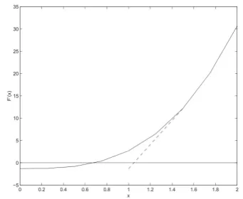
Figure 1. Geometric explanation of Newton’s method
situation, an iterative method is often employed to solve the problem. The iterative method constructs a sequence of points xk, k = 0,1,2, ..., so that it converges to a solution of the problem. The points xk are considered as approximations of a solution to the problem. In practical applications, we stop the calculations at some iteration k
and we accept xk as a sufficiently good approximation of a solution. It is clearly the first thing to be addressed, although the condition is neither necessary nor sufficient for a convergent iterative method.
A wide class of problems which arises in various disciplines can be formulated by the nonlinear equations of the form f(x) = 0.
The Newton’s method [13], [15] is one of the best iterative methods for solving a single nonlinear equation by using the formula
xn+1=xn− f(xn)
f0(xn) (4)
which converges quadratically in some neighborhood of
x∗. It is well known that Newton’s method has a problem that the condition f0(x)6= 0 in a neighborhood of root
x∗ is severe for its convergence.
The algorithm can be viewed as using the tangent to the curve of f0(x)to predict where f(x)itself becomes zero (see Fig. 1).
The iterations of the method generatexk+1as a
station-ary point of the quadratic function defined by the values of f(xk),f0(xk)andf00(xk). Another method is a direct search iterative method based on locating the minimum of the quadratic defined by values of f at three points
xk, xk−1, xk−2 and a gradient approach could minimize the local quadratic approximation of f(xk−1),f0(xk−1) and f(xk). If a minimum xk+1 is found close enough to x∗, then the iteration terminates; otherwise xk+1 is used to generate a new quadratic model to predict a new minimum.
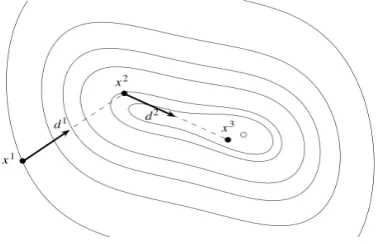
To choose a direction dk and then to make a step in this direction, we set xk+1 =xk+τkdk with some step size coefficient τk >0. This process is illustrated in Fig. 2. After this step, a new direction dk+1 can be chosen at
Figure 2. Moving directions
The cases where the interpolated quadratic has negative curvature and thus does not have a minimum must be treated in the practical implementation of this basic idea. To locate a group of points which implies a suitable quadratic model, the bracketing algorithm is often used. Another method is based on the repeated location of the minimum of a cubic polynomial fitted either to values of
f at four or two points. Although the method is often fast, it also must avoid the search attracted to a maximum of the interpolating polynomial.
Many iterative methods with cubic convergence have been developed in recent years. However, these modified Newton’s methods also suffer the problem which restricts their applications. The research of the new methods free from the restriction of derivatives are required for practical applications.
Continued fractions have a long history and applica-tions. The origin of the continued fractions may be placed in the age of Euclid’s algorithm for the greatest common divisor [14], [15]. Continued fractions experience a revival nowadays thanks to their applications in high speed com-puter arithmetics. Faster division and multiplication, fast and precise evaluation of functions, precise representation of transcendental numbers are the advantages of continued fractions in computer arithmetics.
We can give some basic definitions and results here. The integer part of a real number xis denoted asbxc.
Definition 1: (an)n∈N, the continued fraction
expan-sion of a real numberxcan be obtained by the following algorithm
x0=x, an=bxnc, xn+1=
1
xn−an ifxn6∈Z, 0 otherwise.
Where a0 ∈Zand an ∈N. The algorithm producing
the continued fraction is closely related to the Euclidean algorithm for computing the greatest common divisor of two integers. It is thus readily seen that if the numberxis rational, the algorithm eventually produces zeroes. There existsN ∈Nsuch that an = 0for alln > N, and thus
x=a0+ 1
a1+ 1
a2+ 1
. ..+ 1
aN−1+
1
aN
(5)
We write x= [a0, . . . , aN]. On the other hand, if we
want to find an expression with a0 ∈ Z and otherwise an ∈N\ {0}, the continued fraction[a0, . . . , aN]and
x=a0+ 1
a1+
1
a2+
1
. ..+ 1
aN−1+
1
(aN −1) +1 1 If the numberxis irrational, then the sequence of the so called convergent
a0, a0+ 1
a1, . . . , a0+
1
a1+ 1
a2+ 1
. ..+ 1
an−1+ 1
an
(6)
converges to x for n → ∞. On the other hand, every sequence of rational numbers with a0 ∈ Z and an ∈ N\ {0} converges to an irrational number. We writex=
[a0, . . . , an, . . .].
Letx∈R\Qand let pqnn be itsn-th convergent (where
pnandqnare coprime) and let pq withp, q∈Zbe distinct
from pn
qn and such that0< q≤qn. Then
x−pn
qn
<
x−p
q .
How well the continued fractions approximate irra-tional numbers is also to be treated.
Letx∈R\Qand let pn
qn be itsn-th convergent (where
pn andqn are coprime). Then either
x−pn
qn
< 1
2q2 n
or
x−pn+1
qn+1
< 1
2q2 n+1
.
Continued fractions can get very close to irrational numbers in a certain way.
Letx∈R\Qand let pq withp, q∈Zsatisfy|x−p q|< 1
2q2. Then p
q is a convergent ofx.
The convergent of continued fractions is closely related to the so-called continuantKn(x1, . . . , xn).
Let x0∈R, xi>0, i∈N. Then it holds
x0+ 1
x1+ 1 . ..+ 1
xn
=Kn+1(x0, x1, . . . , xn)
where the polynomial Kn(x1, . . . , xn) is given by the recurrence relation K−1 = 0, K0 = 1 and for n ≥ 1 Kn(x1, . . . , xn) = Kn−2(x1, . . . , xn−2) +
xnKn−1(x1, . . . , xn−1).
For every n∈Nandx1, . . . , xn∈R, we have Kn(x1, . . . , xn) =Kn(xn, . . . , x1).
Let [a0, . . . , an, . . .] be the continued fraction of an irrational numberx. Then itsn-th convergent pn
qn satisfies
pn=Kn+1(a0, . . . , an), qn =Kn(x1, . . . , xn).
III. THEDESIGN OF THEALGORITHM
Let f ∈ C(1)[a, b], y(x) = f0(x). The algorithm we
want are going to design will find x∗ ∈(a, b)such that
y(x∗) = f0(x∗) = 0. If we are given n approximated valuesx0, x1,· · ·, xn−1 ofx∗and the function f and its corresponding derivatives yi=y(xi),0≤i < n.
To find the real roots of y, The following scheme of
npoints based on the continued fraction interpolation of
y=f0(x)can be constructed as follows.
ψ(y) =a0+ y−yn−1
a1+
y−yn−2
. .. y−y2
an−2+ y−y1
an−1
(7)
The kth order difference of function f can be defined recursively as follows.
Φ0(y) =x
Φk(y1,· · ·, yk, y) = y−yk
Φk−1(y1,· · ·, yk−1, y)−Φk−1(y1,· · ·, yk) ,
k= 1,2,· · ·
(8)
It follows from the continued fraction interpolation condition ψ(yi) =xi,0≤i < nthat
a0=xn−1= Φ0(yn−1) ai= Φi(yn−1,· · ·, yn−i−1), i= 1,2,· · · , n−1
(9)
It follows that
ψ(0) =a0− yn−1
a1− yn−2
. .. y2 an−2−
y1 an−1
(10)
According to the formula described above, we can design a very simple iteration algorithm to find x∗ as
follows.
Algorithm III.1: CONTINUED-FRACTION(f)
input x0,· · ·, xn−1, ε
for i←0 to n−1
do yi←f0(xi)
while yn−1> ε
do
g(yn−1,· · · , y1) xn←a0−
yn−1 a1−
yn−2
. .. y2 an−2− y1
an−1 yn←f0(xn)
n←n+ 1
output (xn, yn, f(xn))
where the functiong(yn−1,· · · , y1)is used to compute
the coefficients a0,· · · , an−1 according to the formula
(9).
IV. THECONVERGENCE
Supposef ∈C(1)[a, b], x∈[a, b].
If forxi∈[a, b],0≤i≤k, the limit
lim
x0,···,xk→x
Φk(f0(x0),· · ·, f0(xk)) = Φk(x)
exists, then the functionf iskth inverse differentiable and Φk(x)is called the kth inverse derivative off atx.
Let x∗ ∈ [a, b] and f0(x∗) = 0. The function type
T(n)[a, b]⊆C(1)[a, b]can be defined as
T(n)[a, b] =
{f |f kth inverse differentiable in [a, b],
Φk(x∗)6= 0,1≤k≤n}
If for any function f ∈ T(n)[a, b], the point sequence generated by algorithm 2.1 is{xk}∞1 . We knowxk+1can
be formulated as
xk+1=a0− yk
a1− yk−1
. .. yk−n+3 an−2−yk−n+2
an−1
(11)
wherea0=xk = Φ0(yk), and
ai= Φi(yk,· · · , yk−i), i= 1,2,· · · , n−1.
Then+ 1point inverse continued fraction interpolation of y=f0(x) atx∗, xk−n+1,· · ·, xk can be computed as
follows
ψ1(y) =a00+
y−yk a01+ y−yk−1
. .. y−yk−n+3 a0n−2+ y−yk−n+2
a0n−1+y−yk−n+1
a0 n
(12) It follows from the inverse interpolation condition
It follows that
ψ1(0) =a0−
yk a1−
yk−1
. .. yk−n+2 an−1−yk−n+1
a0 n
=x∗ (13)
Denote x∗= Pn
Qn, and xk+1=
Pn−1
Qn−1. It is not difficult to see that
|xk+1−x∗|=
Pn−1 Qn−1 − Pn Qn = n Y i=1 yk−n+i
|Qn−1Qn|
It follows that
|xk+1−x∗|=
n Y
i=1
|xk−n+i−x∗|
n Y i=1
Φ1(yk−n+i,0)
Qn−1Qn (14) where Qn−1 andQn cab be calculated recursively as
follows
Q−1= 0 Q0= 1
Qi=aiQi−1−yk−i+1Qi−2, i≥1
(15)
ai= Φi(yk,· · ·, yk−i) 1≤i < n an= Φn(yk,· · ·, yk−n+1,0)
(16)
Theorem 1: Letf ∈Tn[a, b]. There must be >0and δ1 > 0 such that when {xk−n+1,· · ·, xk} ⊂ o(x∗, δ1),
|Qn−1Qn| ≥ε.
Proof.
It follows from f ∈Tn[a, b]that
Φk(x∗)6= 0,1≤k≤n.
Therefore, there must beδ1>0,m1>0andM1>12
such that when
{xk−n+1,· · · , xk} ⊂o(x∗, δ1),
0< m1≤ |Φi(yk,· · ·, yk−i)|=|ai| ≤M1,
and
|yk−i+1| ≤ m1
2
m1
4M1 n
,1≤i≤n.
It can be proved by induction that
m1
2
i
≤ |Qi| ≤(2M1)i,1≤i≤n (17) For the case ofi= 1 we have,
m1
2
≤m1≤ |Q1| ≤M1≤2M1.
If the formula (17) is true for the case of i≤R. In the case of i=R+ 1, we have,
QR+1=|aR+1QR−yk−RQR−1| ≤ |aR+1||QR|+|yk−R||QR−1|
≤M1(2M1)R+M1(2M1)R−1≤(2M1)R+1
and
QR+1≥ |aR+1||QR| − |yk−R||QR−1|
≥m1 m21 R
−m1 2
m
1 aM1
R
(2M1)R−1
≥m1 m1 2
R
−m1 2
m1 aM1
R
(2M1)R
= m1
2 R+1
By induction we know that the formula (17) is true for
k= 1,· · ·, n. Therefore,
|Qn−1Qn| ≥ m1 2
n−1 m1 2
n
= m1
2 2n−1
,ε >0
Theorem 2: Let f ∈ Tn[a, b]. There must be δ > 0
such that when{x0,· · · , xn−1} ⊂o(x∗, δ), the sequence
{xk}∞
1 generated by the algorithm 2.1 converges tox∗.
Proof.
It follows from Theorem 1 that there exist >0 and
δ1>0andM1>1/2 such that when
{x0,· · ·, xn−1} ⊂o(x∗, δ1),
|Φ1(yi,0)| ≤M1,0≤i < n, and|Qn−1Qn| ≥ε.
If we set M = M1n
+ 1, then it follows from formula
(14) that when
{x0,· · ·, xn−1} ⊂o(x∗, δ1),
|xn−x∗| ≤M n−1
Y
i=0
|xi−x∗|.
Take0< δ <min{δ1, n−11√
M}, we then have when
{x0,· · ·, xn−1} ⊂o(x∗, δ),
|xn−x∗| ≤M n−1
Y
i=0
|xi−x∗| ≤M δn< δ,
and thusxn∈o(x∗, δ).
It follows by induction that
{xk}∞1 ⊂o(x∗, δ)⊂o(x∗, δ1).
On the other hand, it follows from Theorem 1 that
|xk+1−x∗| ≤M n Y
i=1
|xk−i+1−x∗|, k ≥n (18)
Thus
|xk+1−x∗| ≤M δn−1|xk−x∗| ≤(M δn−1)k, k ≥n.
It follows from M δn−1 <1 that lim
k→∞|xk−x ∗|= 0.
V. THECONVERGENCERATE OF THEALGORITHM
Theorem 3: The equation
fn(x) =xn−xn−1− · · · −x−1 = 0,(n >1) has a unique positive root τn, and
1< τn< τn+1<2, lim
n→∞τn= 2.
Proof.
Since fn(1) = 1−n < 0 and fn(2) = 1 >0, there
exists τn ∈ (1,2) such that fn(τn) = 0. By Descartes’
sign-rule we know that the number of positive roots of the equation fn(x) = 0 is p ≤ 1 due to the change of signs of the coefficients of fn(x).
In view of the fact thatτnis a positive root offn(x) = 0, we know p= 1. This meansfn(x) = 0has a unique positive root τn, and1< τn<2.
Since
fn+1(τn) =τnfn(τn)−1 =−1<0
andfn+1(2) = 1>0,fn+1(x) = 0has a root in(τn,2), i.e.
1< τn< τn+1<2 (19)
Therefore the sequence {τn} is monotone increasing and bounded above.
Let lim
n→∞τn = τ. Then τ ≤ 2. Now, we will show τ = 2.
Ifτ <2, then for a sufficiently largen we have
fn(τ) =τn−τn−1− · · · −τ−1 =τn−τn−1
τ−1
= (τ−2)ττ−1n+1 <0
We have already hadfn(2) = 1>0. Thus,τn∈(τ,2). That meansτn > τ. This contradicts the fact that τn is monotone increasing and tends toτ.
Thereforeτ = 2.
Theorem 4: Let ω be an iteration procedure and let
C(ω, x∗)be the set of the sequences which converges to
x∗and is produced by ω.M is a positive constant. If for any {xk} ∈C(ω, x∗), there is a positive integerk0 ≥n
such that
kxk+1−x∗k ≤M n Y
i=1
kxk−i+1−x∗k
when k ≥ k0, then OR(ω, x∗) ≥ τn, where τn is the
unique positive root of the equation
fn(x) =xn−xn−1− · · · −x−1 = 0.
Proof.
Set k=kxk−x∗k.
Then for allk≥k0,k+1≤M k· · ·k−n+1. Set ηk =M
1 n−1ε
k. Then,
ηk+1≤ηkηk−1· · ·ηk−n+1 (20)
Since k →0, there exists a positive integer k0 and a
positive number η such that for all k≥k0,ηk ≤η <1.
Now, we will show by induction that
ηk0+i≤ηµi, i= 1,2,· · · (21)
whereµiare defined by the following difference equa-tion:
µ1=µ2=· · ·=µn= 1
µi+1=µi+µi−1+· · ·+µi−n+1, i=n, n+ 1,· · ·
(22)
Fori= 1,2,· · · , n, the formula(21)is trivial. Let the formula(21)is true forn≤m≤i. Then wheni=m+1, it follows from the formula (20)that
ηk0+m+1≤ηk0+m· · ·ηk0+m−n+1≤ηµm+···+µm−n+1 By induction we know that the formula(21)holds. Now, we will show µi satisfy
µi≥ατni, i= 1,2,· · · (23)
whereα=τn−n.
In fact, since τn > 1, the formula (23) is obviously true for i= 1,2,· · ·, n. Suppose the formula(23)holds when n≤m≤i. Then when i=m+ 1,
µm+1=µm+µm−1+· · ·+µm−n+1
≥α(τm
n +τnm−1+· · ·+τnm−n+1)
=ατnm−n+1(τnn−1+τnn−2+· · ·+τn+ 1)
=ατnm−n+1τn
n =ατnm+1
By induction we know that the formula (23) holds. Therefore,
εk0+i=M 1
1−nηk0+i≤M 1 1−nηατni It follows that
Rτn{xk}= lim sup
i→∞ ε
1 τnk0+i
k0+i ≤η α τnk0 <1
Thus for any ε >0,Rτn−{xk}= 0.
Therefore,OR(ω, x∗)≥τn.
Theorem 5: Let ω be the iteration procedure formed by the inverse continued fraction interpolation algorithm 2.1 and f(x) satisfy the conditions of Theorem 2. Then
OR(ω, x∗)≥τn, whereτn is the unique positive root of
the equation
fn(x) =xn−xn−1− · · · −x−1 = 0.
Proof.
It follows from Theorem 2 that when
{x0,· · ·, xn−1} ⊆o(x∗, δ), the sequence{xk} produced
by the algorithm 2.1 converges tox∗. From the proof of Theorem 2 we know that (18) holds. Therefore, {xk}
satisfies all conditions of Theorem 4. By Theorem 4 we conclude thatOR(ω, x∗)≥τn.
VI. EXPERIMENTS ANDAPPLICATIONS
If the convergence order η of an iterative method is given as
lim
n→∞
|en+1|
|en|η =c >0
TABLE I.
COMPARISON OF THE PRESENTED METHOD ANDNEWTON’S
METHOD
Equations Iterationsk Presented method Newton’s method
f1(x) = 0
3 1.3×10⁻⁵ 4.3×10⁻¹
4 5.1×10⁻¹³ 4.2×10⁻³
5 5.5×10⁻²⁴ 7.5×10⁻⁴
6 1.2×10−49 2.5×10⁻⁷
7 2.7×10−97 2.3×10⁻¹³
8 3.3×10−196 1.7×10⁻²⁸
9 2.3×10−390 1.3×10−55
f2(x) = 0
4 8.9×10⁻⁹ 7.5×101
5 1.7×10⁻¹⁶ 2.6×101
6 1.5×10⁻³³ 9.7×100
7 3.6×10−66 3.3×100
8 6.8×10−133 9.3×10⁻¹
9 8.7×10−625 1.6×10⁻¹
15 - 5.3×10−75
f3(x) = 0
4 8.6×10⁻⁷ 1.5×10⁻³
5 7.7×10⁻¹⁴ 4.2×10⁻⁴
6 4.8×10⁻²⁷ 1.2×10⁻⁴
7 2.3×10−54 2.5×10⁻⁵
8 5.8×10−108 6.3×10⁻⁶
9 3.5×10−216 1.5×10⁻⁶
90 - 2.6×10−56
ρ=ln|(xn+1−γ)/(xn−γ)| ln|(xn−γ)/(xn−1−γ)|
In this section, we consider the equations on each given interval and initial points as below for numerical performance experiment of our new algorithm.
f1(x) =xsinx+ cosx−0.6, x0= 0
f2(x) = 1 + (x−2)e−x, x0= 0
f3(x) =esinx−x−1, x0= 1
(24)
All the computations are carried out using the C++ programming language. Many scientific computations de-mand a very high degree of numerical precision [13], [15]. For convergence, it is required that the distance of two consecutive approximations|xn+1−xn|be less than
. And, the absolute value of the function |f(xn)| also
referred to as residual be less than .
In the numerical implementation for the examples above, a stopping criterion |f(xn)| < for a small
number = 10−500 within a maximum number of iterationskmax= 100is used.x0 =b, the right endpoint
of the given interval is taken as the initial approximation for the Newton’s method. The numerical results of the values |f(xk)| for the approximations obtained by the presented method and the Newton’s method are presented in Table 1. The sign ”-” in the Table 1 indicates that the corresponding iteration is stopped as the approximation
|f(xk)| satisfies the criterion |f(xk)| < . Our new method is superior to the Newton’s method as shown in Table 1. The convergence rate of the Newton’s method seems to be very slow for the equations fi(x) = 0, i= 2,3.
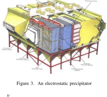
We have also applied our new algorithm to a project of optimal design of the noumenon structure of the
largełs-Figure 3. An electrostatic precipitator
Figure 4. The structure and size of the wall
cale electrostatic precipitator. The noumenon structure of a largełscale electrostatic precipitator is shown in Fig. 3. There are five parts of the structure, including the collecting electrode system, corona electrode system, the housing system, smoke box discharging systems and storage systems. The goal of our project is to optimized the noumenon structure of the electrostatic precipitator, to get a more rational structure, lighten the weight, save the material and reduce the costs.
Our new algorithm is used in the structural optimization of the wall of an electrostatic precipitator with good results. The wall of the electrostatic precipitator is made up of A3 steel plates and steel bars. Its size is shown in
Fig. 4. Its main loads are the negative pressures vertically distributed over the wall. The goal is to find a minimum weight design subjected to the stress constraints σi ≤σ
and the deflection constraints wi ≤w. If we divide the wall along the Y axis properly into n points, then we can set a boolean variable xi to each divided points. If
xi = 1 we then put a bar parallel to the X axis at the point i. Otherwise, ifxi = 0 then no bar at the point i. The design variables can be expressed as a binary n-vector
X = (x1,· · ·, xn), and the problem can be formulated as a nonlinear programming problem as follows.
minZ(X) =kXk=Pn i=1xi
s.t.
σi−σ≤0 , i= 1,· · · , m wi−w≤0 , i= 1,· · · , m x1=xn= 1 ,
xi∈ {0,1} , i= 1,· · · , n
(25)
local line search algorithm to solve the above nonlinear programming problem. The final optimal design makes an originally unfeasible design become a feasible design and reduce the total weights by47.8%.
VII. CONCLUDINGREMARKS
New algorithms and theoretical techniques for solving nonlinear equations have been developed and their ap-plications have been expanding at an astonishing rate in all directions during the last few decades. The constantly increasing emphasis on the interdisciplinary nature of the field is the most striking trends in optimization. In all areas of applied mathematics, engineering, medicine, economics and other sciences, optimization has been a basic tool nowadays. In these areas, to develop iterative methods for solving nonlinear equations has become more and more important. There are some progress about multi step methods in the recent years. These multi step methods have been developed by combining the Newton’s method with other optimization methods.
In this paper, we have proposed an efficient algorithm for solving the nonlinear equations. The presented new algorithm has a fast convergence rate. In general, the scheme of n = 3 with a convergence rate τ3 = 1.8393
or n= 4with a convergence rate τ4= 1.9276converges already very fast.
The computational experiments demonstrate that the achieved results are not only of theoretical interest, but also that the techniques developed may actually lead to considerably faster algorithms.
ACKNOWLEDGEMENT
The authors acknowledge the financial support of Natural Science Foundation of Fujian under Grant No.2013J0101, and the Haixi Project of Fujian under Grant No.A099. The authors are grateful to the anony-mous referee for a careful checking of the details and for helpful comments that improved this paper.
REFERENCES
[1] S. Amat, C. Bermudez, S. Busquier, S. Plaza, On two families of high order Newton type methods,Appl. Math. Lett., vol. 25, no.12, pp. 2209-2217, 2012.
[2] S. Amat, S. Busquier, A. Grau, M. Grau-Sanchez, Max-imum efficiency for a family of Newton-like methods with frozen derivatives and some applications,Appl. Math. Comput., vol. 219, no.15, pp. 7954-7963 , 2013.
[3] Michael Bartholomew-Biggs,Nonlinear Optimization with Financial Applications, Kluwer Academic Publishers, New York, 2005.
[4] J. Dzunic, M.S. Petkovic, L.D. Petkovic, Three-point methods with and without memory for solving nonlinear equations,Appl. Math. Comput., vol. 218, no.9, pp. 4917-4927, 2012.
[5] J.A. Ezquerro, M. Grau-Sanchez, A. Grau, M.A. Hernan-dez, M. Noguera, N. Romero, On iterative methods with accelerated convergence for solving systems of nonlinear equations,J. Optim. Theory Appl., vol. 151, no.1, pp. 163-174, 2011.
[6] M.A. Hernandez, N. Romero, On a characterization of some Newton-like methods of R-order at least three, J. Comput. Appl. Math., vol. 183, no.1, pp. 53-66, 2005. [7] J.A. Ezquerro, M.A. Hernandez, An improvement of the
region of accessibility of Chebyshev’s method from New-ton’s method,Math. Comput., vol. 78, no.1, pp. 1613-1627, 2009.
[8] Fang L., A cubically convergent iterative method for solving nonlinear equations, Adv. Appl. Math. Sci., vol. 10, no. 2, pp. 117-119, 2011.
[9] M. Grau-Sanchez, A. Grau, M. Noguera, Frozen divided difference scheme for solving systems of nonlinear equa-tions,J. Comput. Appl. Math., vol. 235, no. 6, pp. 1739-1743 2011.
[10] M. Grau-Sanchez, A. Grau, M. Noguera, On the compu-tational efficiency index and some iterative methods for solving systems of nonlinear equations,J. Comput. Appl. Math., vol. 236, no. 6, pp. 1259-1266, 2011.
[11] Y.I. Kim, Y.H. Geum, A cubic-order variant of Newton’s method for finding multiple roots of nonlinear equations,
Comput. Math. Appl., vol. 62, no. 4, pp. 1634-1640, 2011. [12] M.S. Petkovic, J. Dzunic, B. Neta, Interpolatory multipoint methods with memory for solving nonlinear equations,
Appl. Math. Comput., vol. 218, no. 6, pp. 2533-2541, 2011. [13] L.B. Rall, Computational Solution of Nonlinear Operator Equations, Robert Krieger Publishing Company, Inc., Cal-ifornia, 1979.
[14] F. Sha, X. Tan, A class of iterative methods of third order for solving nonlinear equations,Int J. Nonlinear Sci., vol. 11, no. 2, pp. 165-167, 2011.
[15] J.F. Traub,Iterative Methods for the Solution of Equations, Chelsea Publishing Company, New York, 1977.
[16] X. Wang, L. Wang, A Fast Algorithm for Solving Nonlin-ear Equations, International Conference on System Mod-eling and Optimization (ICSMO 2012), pp. 6-9, 2012. [17] T. Yamashita, H. Yabe, T. Tanabe, A globally and
super-linearly convergent primal-dual interior point trust region method for large scale constrained optimization, Math. Program. Ser. A, vol. 102, no. 1, pp. 111-151, 2005. [18] B. I. Yun, Solving nonlinear equations by a new derivative