A Parallel Preconditioned Bi-Conjugate Gradient
Stabilized Solver for the Poisson Problem
Zhao Ninga,b
a.College of Geophysics,ChengDu University of Technology ,ChengDu,China b.School of Computer Science and Technology,Henan Polytechnic University
Email: [email protected]
Wang XuBen
Key Lab of Earth Exploration&Information Techniques of Ministry of Education .ChengDu University of Technology ,ChengDu,China
Email: [email protected]
Abstract—We present a parallel Preconditioned
Bi-Conjugate Gradient Stabilized(BICGstab) solver for the Poisson problem. Given a real, nosymmetric and positive definite coefficient matrix , the parallized Preconditioned BICGstab -solver is able to find a solution for that system by exploiting the massive compute power of todays GPUs.Comparing sequential CPU implementations and that algorithm.we achieve a speed up from 8 to 10 depending on the dimension of the coefficient matrix. Additionally the concept of preconditioners to decrease the time to find a solution is evaluated using the AINV method.
Index Terms—sparse matrix solver, Bi-Conjugate Gradient
Stabilized, ELLPACK-R, NVIDIA CUDA, AINV precondition
I. INTRODUCTION
Compared to the classical CPU environments, The graphics processors play an important role in parallel and distributed systems. The floating point processing provides general purpose computations on GPGPU. For this reason,numerical calculation can be accelerated as long as the algorithms well to the characteristics of the hardware. In communication-and bandwidth-limited problems, The algorithm for solving large-scale sparse group of linear equations causes negative speedups. Our job aim to the Poisson problem that arises in a large range of disciplines like gravity,magnetic,electrical,and seismic [1]. The numerical calculation result of mass data discretization must be processed by the system, especially in three dimension compute. Thus, Iterative solution usually instead of direct solution.
T h e iter a tive me th o d s ar e mo r e a me n a b le to parallelism and therefore can be used to solve larger problems. Currently, the most popular iterative schemes belong to the Krylov subspace family of methods. They include Preconditioned Bi-Conjugate Gradient Stabilized (BiCGSTAB) and Preconditioned Conjugate Gradient
(CG) iterative methods for nonsymmetric and symmetric positive definite (s.p.d.) linear systems.In practice, we often use a variety of preconditioning techniques to improve the convergence of iterative method. In this paper we focus on the Approximate Inverse(AINV) preconditioning for the numerical simulation [2]. The preconditioned Bi-Conjugate Gradient Stabilized was introduced in as an efficient method to solve linear equation systems with real, symmetric and positive definite coefficient matrices. With the appearance of programmable graphics hardware a cheap way for getting massive parallel processors to the masses became possible. Therefore, general people can also take advantages from parallel algorithms. When analysing the conjugate gradient algorithm one will recognize that serveral operations within one iteration of the algorithm can be computed in parallel. In a parallel implementation was introduced using GLSL shader programs. The necessary data for the computation was stored in textures and the algorithm was implemented in a pixel shader. Due to the general purpose GPU paradigm encoding of data in textures got superfluous because new technologies, like the NVIDIA CUDA architecture allow programming the parallel processors using an extended version of the C programming language.If one wants to reach a time efficient implementation of the Preconditioned Bi-Conjugate Gradient Stabilized. it is essential to have an efficient way to compute sparse matrix vector products. In an efficient storage for sparse matrices the ELLPACK format was suggested, which was extended to the ELLPACK-R format in especially for the use on GPUs. For time efficient solution of linear systems it is not enough to have efficient data structures and a lot of compute power: There exist extensions to the conjugate gradient algorithm which use a preconditioning matrix which is applied to the system matrix to decrease its condition number. In this paper a sequential version of such preconditioner is evaluated using the AINV method described in .
A. The Poisson Equation and its Applications
The Poisson equation is a second-order partial differential equation that arises in a large range of electrical problems[3]. Its common form is
(1)
Δ =
φ
f
where
Δ
denotes the Laplacian. In three-dimensional Cartesian coordinates, the Poisson equation can express as:(2)
2 2 2
2 2 2
f
x
y
z
φ
φ
φ
∂
+
∂
+
∂
=
∂
∂
∂
Analytic Method for the Poisson equation are usually not operate. A general approach is to discretize the domain into a finite number of grid points.Discretization schemes for partial differential equations such as the Finite Difference, the Finite Element, or the Finite Volume scheme ultimately lead to the need for the solution of a large system of linear equations. Since the coupling between the equations is usually rather weak, the system matrix is very sparse, allowing for millions of unknowns on average workstations[4]. For such huge systems, iterative solution methods are typically employed, where the convergence rate depends on the condition number of the iteration matrix. Consequently,in practical applications it is of interest to keep the condition number low, for which so-called preconditioners are employed. Formally, one way of interpreting the action of a preconditioner is to multiply the original system ,as in (1) .
A
•
X
=
B
(1) For example, An Finite Difference Frequency Domain method solves Maxwell's equations,where A is a nosymmetric complex matrix. The matrix A depends onthe conductivities and grid spacings, b is a vector containing source terms associated withthe boundary conditions, and x is the unknown complex vector of the electric field components throughout the model.Nowadays, the system is commonly solved iteratively by a preconditioned Krylov method . In this respect, only two aspects are important, first, how accurate the systemA
•
X
=
B
, and second, how well-preconditioned the system matrix A is .B. The Preconditioned Bi-Conjugate Gradient Stabilized In last several years, a number of Krylov subspace algorithms have been proposed for processing linear systems.These methods proceed in an iterative manner to minimize,as in (2).
r = Ax-b (2) The error is not reduced at each iteration,and thus the convergence is generally erratic,these techniques have proven successful in reducing the error to a predetermined level within an acceptable number of iterations.The most largely used of the techniques is the preconditioned Biconjugate Gradient Stabilized (BiCGSTAB)method for electromagnetic modeling by Sarkar and recently for magnetotelluric modeling by smith[5].The pseudocode for the preconditioned BiCGSTAB iterative method is shown in Alg. 1.
( )
( )
( )( )
( )
0 0
0 0 0
0 0
0 0
0 1
1 1
1 1 1 1
1
1.
2. Choose an arbitrary vector such that , 0
3. 1
4. 0 5. For 1, 2, 3,
1. ,
2. / /
3.
4.
5.
i i
i i i
i i i i i
i i
r b Ax
r r r
v p i
r r
p r p v
y K p v ρ α ω ρ β ρ ρ α ω β ω − − − − − − − − = − ≠ = = = = = = … = = = + − = = ( )
(
)
0 1 11 1 1 1
1
6. / ,
7.
8.
9.
10. (K , ) / ,
11.
12. If is accurate enoughthen quit 13.
i i
i i
i
i i i
i
i i
Ay
r v
s r v
z K s t Az
t K s K t K t
x x y z
x
r s t
α ρ α ω α ω ω − − − − − − − = = − = = = = + + = −
Algorithm 1. Preconditioned BiCGSTAB C. AINV Preconditioning Techniques
One approach to advance stability and acceleration is the preconditioning of the coefficient matrix A. The cgalgorithm converged much faster for coefficient matrices with smaller condition number.
The computational complexity of preconditions is far lower than for handling 1
A− process.It is to transform Ax = b into an equivalent system, and the coefficient matrix condition number is far less than the cond (A) linear algebraic equations.The equivalent system of linear equations select the appropriate commonly used iterative method,. At this time, due to the coefficient matrix of the condition number is small[6],The iteration method of convergence fastly reach the purpose of accelerated iteration.The precondition of Incomplete Factorization or SSOR are well suitable for cpu processing and can greatly reduce the computating time. However, these preconditioners are unfit for GPU architectures. The Approximate Inverse (AINV), which is to find an
1 1
M − ≈ A− directly without going the detour through an approximation of A.,is a good choice.
Based on the matrix decomposition, sparse approximate inverse with Krylov subspace methods has many advantages,If A is symmetric positive definite matrix,the precondition of symmetric positive definite can keep coefficient matrix. After pretreatment of linear system can use the CG method to solve. Compared to other approximate inverse algorithm, it has a small amount of calculation and the parameters,so that to reduce the uncertainty of the system.
AINV algorithm provided by Benzi et al.In order to keep sparsity ,we consider a program based on a direct method of matrix inversion. This lead to a factorized sparse G ≈ A−1 .
Our preconditioner is based on an algorithm which computes two sets of vectors{ } 1
n i i
Z = ,{ } 1 n i i
A-biconjugate, such that 0
T
i j
w A z =
if i ≠ j. Given a matrix A∈ Rn×n ,Between the problem of inverting A
and that of computing two sets of A-biconjugate vectors
1
{ }n i i
Z =
,
{ }
1 n i iw
==1 .
It computes two sets of vectors{ } 1 n i i
Z = ,{ }n1 i i
W =
,If we introduce the matrices:
1, 2
[ , ,..., ]
nZ
=
z z
z
and
W
=
[ , ,..., ]
w w
1, 2w
n , then1 2
( , , ..., )
T
n
W A Z =D =d ia g p p p ,
Where pi = w A ZiT i ≠ 0 . It follows W and Z are necessarily nonsingular and
1 1
1
T n T i i
i i
z w
A ZD W
p
− −
=
= =
∑
Therefore, A has an LU factorization, Z can be computed make use of a biconjugation process applied to the basis vectors e e1, 2, ...en .It is easily observed that
1
Z =U− and W = L−T
whereA = L D U which L and U
lower and upper triangular and D diagonal.If
T i
a
denotes
the i row of A,Ciis the i column of A, the biconjugatioin
procedure to compute Z can be written as follows[7]:
○1 Let
0 0
1 1, 1 11
z =e p =a
○2 for i=2,...,n,do
○3
0
i i
z =e
○4 for j=1,2,...,i-1,do
○5
1: 1
j T j i j i
p − =a z −
○6
1
1 1
1
:
j
j j i j
i j j j
j
p
z a z
p
−
− −
−
⎡ ⎤
= − ⎢ ⎥
⎢ ⎥
⎣ ⎦
○7 end do
○8 pii 1: a ziT ii 1 − = −
○9 end do
Algorithm2. AINV algorithm
If pi is a negative or zero value. Benz pointed out that
: T 0
i i i
p = z A z > .However,if A is an symmetrical matrix.
the resulting SAINV preconditioner is general extremely effective[8] . In general , accuracy zero is very impossible to occur , resulting in uncontrolled growth of the entries of Z and W. So as to avoiding the happening of fault, by analyzing the reason of pivots may be negative or zero value and avoiding them.
The AINV preconditioner consisting of matrix–vector products is easily parallelized on GPU computer. One possible solution is to compute the preconditioner sequentially on one processor and then to allocate factors among processors. Relative to the overall costs, the time for computing the preconditioner is negligible[9].
III.GPUARCHITECTURE AND CUDA
A .GPU Architecture
GPU is built as a scalable array of multi-threaded Streaming Multiprocessors (SMs), each of which consists of multiple Scalar Processor (SP) cores. To manage hundreds of threads, the multiprocessors employs a Single Instruction Multiple Threads (SIMT) model. The NVIDIA GPU platform has various memory hierarchies. The types of memory can be classified as follows: (1) global memory, (2) local memory, (3) on-chip shared memory, (4) read-only cached off-chip constant memory and texture memory and (5) registers. The effective bandwidth of each type of memory depends significantly on the access pattern. Global memory is relatively large but has a much higher latency (from 400 to 800 cycles for the NVIDIA GPUs) compared with the on-chip shared memory (1 clock cycle if there are no bank conflicts).Global memory is not cached, so it is important to follow the right access pattern to achieve good memory bandwidth[10].
Threads are organized in warps. A warp is defined as a group of 32 threads of consecutive threadIDs. A half-warp is either the first or second half of a half-warp. The most efficient way to use the global memory bandwidth is to coalesce the simultaneous memory accesses by threads in a half-warp into a single memory transaction. For NVIDIA GPU devices with compute capability and higher,memory access by a half-warp is coalesced as soon as the words accessed by all threads lie in the same segment of size equal to 128 bytes if all threads access 32-bit or 64-bit words. Local memory accesses are always coalesced. Alignment and coalescing techniques are explained in details in [11].
Since it is on chip, the shared memory is much faster than the global memory but we also need to pay attention to the problems of bank conflict. The size of shared memory is 16K per SM. Cached constant memory and texture memory are also beneficial for accessing reused data and data with 2D spatial locality[12].
B. CUDA Concepts
The parallelization of the algorithm is done using the NVIDIA CUDA technology. This technology makes it possible to exploit the massive compute power of todays GPUs for general purpose computing by creating kernel programs which execute in parallel.
Figure 1: CUDA-programming model
C. Related Work
The potential of GPUs for parallel sparse matrix computations was recognized early on when GPU programming required shader languages. After the advent of NVIDIA CUDA, GPUs have drawn much more attention for sparse linear algebra and the solution of sparse linear systems. Existing implementations of the GPU Sparse matrix-vector product (SpMV) include CUDPP (CUDA Data Parallel Primitives) library [15], NVIDIA CUSPARSE library and the IBM SpMV library . In [16], different formats of sparse matrices are studied for producing high performance SpMV kernels on GPUs.
A GPU-accelerated Jacobi preconditioned CG method is studied in [17].The CG method with incomplete Poisson preconditioning is proposed for the Poisson problem on a multi-GPU platform.The Block-ILU preconditioned GMRES method is studied for solving sparse linear systems on the NVIDIA Tesla GPUs in. SpMV kernels on GPUs and the Block-ILU preconditioned GMRES method are used in for solving large sparse linear systems in black-oil and compositional flow simulations. A GPU implementation of deflated PCG method for bubbly flow computations is discussed in [18].
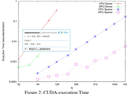
Figure 2: CUDA-execution Time
IV.PARALLELIZED PRECONDITIONED BICGSTAB IN
CUDA
A.Sparse Matrix-Vector Product
In every iteration of the algorithm we have to compute several additions, dot products and a matrix-vector multiplication[19].
The threads of a block are executed as packages of 16 threads which is also called halfwarp. The threads inside a halfwarp are generally running in parallel. The blocks of a compute grid are executed sequentially but in case of available hardware resources blocks are dispatched and executed in parallel to other blocks. Every thread has two information: first in which block it is running and secound by which block internal number it is identified[20]. Hence the numbering of the threads can be done by,as in (2).
int i = blockIdx.x * blockDim.x + threadId.x.(2) This is also illustrated in Figure 1. The next example demonstrates the addition of two vectors implemented in C for CUDA (see Algorithm 3).
global void VecAdd(float* A, float* B, float* C, int n) {
int i = blockIdx.x * blockDim.x + threadId.x; if (i < n) C[i] = A[i] + B[i]
}
Algorithm 3: CUDA-vector addition
The sparse matrix-vector product (SpMV) is one of the major components of any sparse matrixcomputations. However, the SpMV kernel which accounts for a big part of the cost of sparse iterative linear solvers, has difficulty in reaching a significant percentage of peak floating point throughput. It yields only a small fraction of the machine peak performance due to its indirect and irregular memory accesses[21]. Recently, several research groups have reported their implementations on high-performance sparse matrix-vector multiplication kernels on GPUs .NVIDIA researchers have demonstrated that their SpMV kernels can reach 15 GFLOPS and 10GFLOPS in single/double precision for unstructured mesh matrices. This section, will discuss implementation of SpMV GPU kernels using several different formats.
For a matrix-vector product, y = Ax, data reuse can be applied to the vector x which is readonly.Therefore, a good strategy is to place the vector x in the cached texture memory and access it by texture fetching . As reported in , caching improves the throughput by an average of 30% and 25% in single and double precision respectively[22].
B. SpMV in CSR Format
The compressed sparse row (CSR) format is probably the most widely used general-purpose sparse matrix storage format [23]. In the CSR format, the sparse matrix is specified by three arrays: one real/complex data array A which contains the non-zero elements row by row;To parallelize the SpMV for a matrix in the CSR format, a simple scheme called scalar CSR kernel is to assign each row to one thread. The computations of all threads are independent.
coalescing should be higher. But this approach incurs another problem related to computing vector dot products in parallel (dot product of a matrix row vector with the vector x). To solve this problem, each thread saves its partial result into the shared memory and a parallel reduction is used to sum up all partial results. Moreover, since a warp executes one common instruction
at a time, threads within a warp are implicitly synchronized and so the synchronization in the half-warp parallel reduction can be omitted for better performance . In addition, full efficiency of the vector CSR kernel requires at least 16 non-zeros per row in A. Our vector CSR kernel is slightly different from the implementation in which a warp of threads are assigned to each row[24].
C. SpMV in ELL Format
The classical formats to store a sparse matrix (coordinate storage, compressed column storage, compressed row storage) are not applicable to parallelize the matrix vector product . In an efficient storage for sparse matrices the ELLPACK format was suggested, which was extended to the ELLPACK-R format especially for the use on GPUs. A matrix A∈Rn m× is
represented by Nz∈N the maximal number of elements unequal to zero per row,a representation matrix
n N z
A∈ R × for the element unequal to zero,a
representation matrix 0 n N z
j∈ N × for the indice of the elements and an information vector 1 0
n
r ∈ N containing the number of the element per row.For
4 3
4 2
0
1 3 0
0 11
4 00
0 02
2 :
1 3 0 1
11 1 2
,
4 0
2 2
A R
withNz wehavethe following ELLPACK Rrepresentation
A R j N
×
×
⎛ ⎞ ⎜ ⎟ ⎜ ⎟ = ∈
⎜ ⎟ ⎜ ⎟ ⎝ ⎠
= −
⎛ ⎞ ⎛ ⎞ ⎜ ⎟ ⎜ ⎟ ⎜ ⎟ ⎜ ⎟ = ∈ = ∈
⎜ ⎟ ∗ ⎜ ⎟ ∗ ⎜ ⎟ ∗ ⎜ ⎟ ∗ ⎝ ⎠ ⎝ ⎠
4 2 4
0
2
2 , 1
1
1
r N
×
⎛ ⎞ ⎜ ⎟ ⎜ ⎟ = ∈
⎜ ⎟ ⎜ ⎟ ⎝ ⎠
Let A be a matrix in ELLPACK-R representation. We realize the matrix-vector multiplication with n threads as seen in Algorithm 4[25].
: ,
:
0 1
0 m a x 1[ ]
0 m a x 1
[ ]
[ ]
[ ] [
n m m
n
In p u t A R v R O u tp u t u A v R
fo r th r e a d In d e x x to n d o in p a r a lle l s v a lu e
r x
fo r i to d o v a lu e A x in c o l j x in
s v a lu e s v a lu e v a lu e v c o l u x
×
∈ ∈
= ∈
← ← − ←
←
← − ← + ← +
← + ⋅
]← s v a lu e
Algorithm 4: Matrix-vector multiplication in ELLPACK-R format.
The ELL formats are well-suited to matrices obtained from structured grids and semi-structured meshes[26]. CSR is a popular, general-purpose sparse matrix format which is convenient for many other sparse matrixcomputations. CSR kernels are subject to execution divergence caused by variations in the distribution of nonzeros per row.The COO SpMV kernel based on segmented reduction is robust with respect to variations in row sizes and others consistent performance. However, the COO format is verbose and has the worst computational intensity of the formats considered. Furthermore, the segmented reduction operation more expensive than alternative techniques that rely on a simpler decomposition of work into threads of execution. Nevertheless,the COO kernel is reliable and complements the deciencies of the other SpMV kernels(Figure 2).
Figure 3: Exposing Parallelism
A direct implementation of SPAI on GPUs, however, is hampered by the observation that the cardinality of the index sets Ik and Jk cannot be obtained a-priori. Since dynamic memory allocation on GPUs using OpenCL is not possible by now, expensive scans for the required memory would be necessary. Therefore, the index sets Ik and Jk are set up on the CPU and then copied to GPU. After that, the matrices A(Ik,Jk) are set up.The massively parallel architecture of GPUs suggests to solve all Least Squares problems simultaneously.However,overall memory requirements induced by the Least Squares problems may soon exceed the limited GPU RAM, thus only a subset can be processed at the same time. In our implementation the overall memory requirements on the GPU are computed from the size of the index sets Ik and
Jk. If GPU RAM turns out to be too small, the work load is split into two chunks of equal size, which are processed one after another on the GPU. This strategy is then applied in a recursive manner to each of the two chunks.
pattern is as follows[28]:
1. Determine the index sets Ik and Jk for each k = 1, . . . ,n. 2. Compute the memory consumption of the n Least Squares problems and split the work load into chunks. 3. For each chunk, assemble the matrices Ak and compute the solution of the Least Squares problems using QR factorization.
4. Copy the results back to CPU RAM and compute the residuals.
5. If further pattern updates are required, compute the augmented index sets I and J , otherwise go to 8.
6.Assemble the new entries in the augmented Least Squares matrix and compute the solution reusing previous QR factorizations.
7. Go back to 4.
8. Write all entries computed in the chunk to M.
D. Shared Memory and Texture Cache
In this section, To reduce the processing time the coefficient matrix was stored in ELLPACK-R format and the matrix vector operations were parallelized.Another approach to advance stability and acceleration is the preconditioning of the matrix. A sequential implementation of the preconditioned Bi-Conjugate Gradient Stabilized algorithm was implemented to evaluate this.Furthermore, the use of Shared Memory and Texture Cache could accelerate the runtime on older graphics cards[29].
In the implementation, which is described in this paper the input data were copied into the global memory of the graphics card. During the execution, the threads get the required data only from this memory, which is about 512 to 2048 MB on modern graphics hardware[30]. There exists also a comparatively small shared memory (it can also be configured as a L1-cache) and texture cache, which is only about a few KB. The access time to this kind of memory is much shorter (sometimes about a factor in the dimensions of 100) in comparison to the often uncached global memory. Because of the small size in the most cases it is not possible to store the whole coefficient matrix inside of it[31]. Another way to speed up the process is the skillful use of this memory. Therefore, it is necessary to copy parts of data for future calculations from global memory to shared memory and texture cache. In order to achieve an acceleration, this must be constructed so that most of these transfers occur in parallel to the running threads.
IV.EXPERIMENTS
This section provides a comparison of the runtimes of the sequential and the parallel implementation of the preconditioned BICGstab algorithm. As an application the possion equation is solved and different sizes of the n x n-coefficient matrix are chose. When solving a linear system the convergence speed of the conjugate gradient algorithm to compute an acceptably accurate solution strongly depends on the condition number of the system matrix. Therefore,the time per iteration is used for detailed comparison. The runtimes of the presented GPU version in CUDA 4.0.
In order to measure the GPU computation ability, we have used a Intel i7-3770 with 4 GB memory, hosting a NVIDIA Geforce 610M with 2 GB memory. All results using double-precision floating-point data. In most compute results,it is a good precision under 1e-10.All those matrices are available on the Sparse Matrix Florida Collection. Their properties are summarized in Table 1.
TABLE 1
DESCRIPTION OF THE MATRICES USED
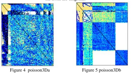
Matrix rows cols nonzero description poisson3Da 13,514 13,514 352,762 nonsymmetric poisson3Db 85,623 85,623 2,374,949 nonsymmetric Figure. 4 Each matrix illustrate the location of the nonzero elements. Some matrices are in close proximity to the diagonal, some elements are
far from the diagonal.
Figure 4 poisson3Da Figure 5 poisson3Db
In Table 2, We minimizes the execution time:ELL format for GPU and CSR format for CPU. The table contains the number of iterations required to reach the threshold condition.
TABLE 2
COMPARISON BETWEEN CPU AND GPU, TIMES IN S Matrix CPU times GPU times iter.
poisson3Da 6.54s 0.68s 81
poisson3Db 167.63 s 20.63 s 288
In Table 3, we inform the amount of floating point computing per second (CPU and GPU). As shown in the fourth column (size, number of nonzero elements,etc.). Solving a linear system in GPU is obviously less efficient than simply computing the SpMV. many operations are not really efficient on GPU.
TABLE3
COMPARISON BETWEEN CPU AND GPU IN GFLOPS
Matrix CPU Gflops
GPU Gflops
% of SpMV in
solving
poisson3Da 0.68 6.11 56
poisson3Db 0.66 7.28 61
V.CONCLUSIONS
CPU implementation using the LAPACK based Armadillo C++ Library 1.0.0 and different CPU implementations was made. In comparisonto the sequential CPU implementations the parallel version of the Bi-Conjugate Gradient Stabilized algorithm is in average 8 to 10 times faster.
ACKNOWLEDGMENT
This work has been supported by National High-tech R&D Program (2009AA06Z108).
REFERENCES
[1] M. Ament, G. Knittel, D. Weiskopf, and W. Strasser.A parallel preconditioned conjugate gradient solver for the poisson problem on a multi-gpu platform. Parallel, Distributed, and Network-Based Processing,Euromicro Conference on, 0:583– 592, 2010.
[2] Michele Benzi.Preconditioning Techniques for Large Linear Systems: A Survey. Journal of Computational Physics 182, 418–477 (2002)
[3] N. Bell and M. Garland. Efficient sparse matrixvector multiplication on CUDA. NVIDIA Technical.Report NVR-2008-004, NVIDIA Corporation, Dec.2008.
[4] Gu Tong-xiang Associate Professor, Doctor, Chi Xue-bin, Liu Xing-ping, Ainv and bilum preconditioning techniques, Applied Mathematics and Mechanics September 2004, Volume 25, Issue 9, pp 1012-1021
[5] J. Georgii and R. Westermann. A multigrid framework for real-time simulation of deformable volumes.In Proceedings of the 2nd Workshop On Virtual Reality Interaction and Physical Simulation,pages 507, 2005.
[6] J. R. GILBERT, Predicting structure in sparse matrix computations, SIAM J. Matrix Anal.Appl., 15 (1994), pp. 62-79.
[7] M. R. Hestenes and E. Stiefel. Methods of conjugate gradients for solving linear systems. Journal of Research of the National Bureau of Standards, 49:409,436, 1952.
[8] Y. Notay, Using approximate inverses in algebraic multilevel methods, Numer. Math. 80, 397 (1998). [9] Y. Notay, A multilevel block incomplete
factorization preconditioning, Appl. Numer. Math. 31, 209 (1999).
[10] NVIDIA-Corporation. Nvidia cuda c programming guide, Version 3.1, 2010.
[11] Y. Saad. Iterative methods for sparse linear systems.Second edition, 2003.
[12] L. N. Trefethen and D. Bau. Numerical Linear Algebra.SIAM: Society for Industrial and Applied Mathematics,1997.
[13] F. Vazquez, E. M. Garzon, J. Martinez, and J. J. Fernandez.The sparse matrix vector product on gpus.aceuales, pages 103, 2009.
[14] R. Freund, A transpose-free quasi-minimal residual algorithm for non-Hermitian linear systems, SIAM J.Sci. Comput. 14, 470 (1993).
[15] M. Benzi and M. Tuma, A sparse approximate inverse preconditioner for nonsymmetric linear systems, SIAM J. Sci. Comput. 19, 968 (1998). [16] M. Benzi and M. Tuma, Numerical experiments
with two approximate inverse preconditioners, BIT 38, 234(1998).
[17] M. Benzi and M. Tuma, A comparative study of sparse approximate inverse preconditioners, Appl. Numer. Math. 30, 305 (1999).
[18] L.Bergamaschi,G.Pini,andF. Sartoretto, Approximate inverse preconditioning in the parallel
solution of sparse eigenproblems, Numer. Linear Algebra Appl. 7, 99 (2000).
[19] George Karypis and Vipin Kumar, Metis – a software package for partitioning unstructured graphs, partitioning meshes, and computing fill-reducing orderings of sparse matrices, version4.0, Tech. report, University of Minnesota, Department of Computer Science / Army HPC Research Center, 1998.
[20] Shubhabrata Sengupta, Mark Harris, Yao Zhang, and John D. Owens, Scan primitives for gpu computing, Graphics Hardware 2007, ACM, August 2007, pp. 97–106.
[21] Nathan Bell and Michael Garland, Implementing sparse matrix-vector multiplication on throughput-oriented processors, SC’09: Proceedings of the Conference on High Performance Computing Networking, Storage and Analysis (New York, NY, USA), ACM, 2009, pp. 1–11.
[22] Serban Georgescu and Hiroshi Okuda, Conjugate gradients on graphic hardware: Performance& Feasibility, 2007.
[23] Rohit Gupta, A GPU implementation of a bubbly flow solver , Master’s thesis, Delft Institute of Applied Mathematics, Delft University of Technology, 2628 BL Delft, The Netherlands,2009. [24] Shubhabrata Sengupta, Mark Harris, Yao Zhang,
and John D. Owens, Scan primitives for gpu computing, Graphics Hardware 2007, ACM, August 2007, pp. 97-106.
[25] Bell N, Garland M (2008) Efficient sparse matrix-vector multiplication on CUDA. NVIDIA technical report NVR-2008-004, NVIDIA Corporation, December 2008
[26] Vasily Volkov and James Demmel, LU, QR and Cholesky factorizations using vector capabilities of GPUs, Tech. report, Computer Science Division University ofCalifornia at Berkeley, 2008.
[27] Mingliang Wang, Hector Klie, Manish Parashar, and Hari Sudan, Solving sparse linear systems on nvidia tesla gpus, ICCS’09: Proceedings of the 9th International Conference on Computational Science (Berlin, Heidelberg), Springer-Verlag, 2009, pp. 864–873.
Conjugate Gradient Solver for the Poisson Problem on a Multi-GPU Platform,"pdp, pp.583-592, 2010 18th Euromicro Conference on Parallel, Distributed and Network-based Processing, 2010
[29] L. Buatois, G. Caumon, and B. Levy, “Concurrent number cruncher: a GPU implementation of a general sparse linear solver,” Int. J. Parallel Emerg. Distrib. Syst., 24(3):205–223,2009. ISSN 1744-5760
[30] Nvidia, “CUDA Toolkit 4.0 CUBLAS Library” NVIDIACorporation, Santa Clara, April, 2011 [31] Nvidia,”CUDA Programming Guide 4.0” NVIDIA