A Novel Algorithm of Edge Location Based on
Omni-directional and Multi-scale MM
Hang Zhou
School of Electronic and Information Engineering, Beijing Jiaotong University Beijing, China
Email:[email protected]
Dan Peng1 and Xin Wang2and Hongyi Wang1
1. School of Electronic and Information Engineering, Beijing Jiaotong University, Beijing, China
2. Telecommunication Signal and Telecommunication Research Institute, China Academy of Railway Sciences,Beijing, China
Email:[email protected]
Abstract—In order to suppress image noise effectively and extract the edge clearly and accurately, a novel approach based on omni-directional and multi-scale mathematical morphology for edge detection is proposed in this paper. In order to compare different object geometries a modified Hausdorff distance application is composed. With a new moments rule used, Opening operation and closing operation of large scale structural elements are adopted for suppression of noise, while small scale structural elements are used for edge extraction. Finally, the weighting combination calculation of edge maps acquired under different directions is executed according to different weights. The experimental results show that the improved algorithm has a great promotion in extracting edge information compared with several reference algorithms.
Index Terms—omni-directional; multi-scale; Hausdorff; edge detection; morphology; structural elements
I. INTRODUCTION
Image edge, which contains image position and contour, reflects the essential visual characteristics of an object. As the first and most important step in the process of geometric object features extraction of digital images, edge detection plays a significant role in computer vision and has important research value in image processing [1-2]. However, due to the complexity of image itself and interference from noise and light shadows, edge extraction is still a conundrum so far. Therefore, the main research directions of edge detection are the presentation of new algorithms or the improvement for pre-existing algorithms [3].
Conventional edge detection algorithms [4] (Sobel algorithm, Roberts algorithm, Prewitt algorithm, etc) show poor performance in anti-noise property and integrity of edge map. Mathematical morphology is an effective method that is widely used in image processing technique. With strict mathematical theory as foundation, it focuses on image geometric relationship and mutual relationship. The algorithm bears the advantage of simple, quick execution speed, parallel processing enabled, easy for hardware realization, etc. When using the traditional
morphology method for edge detection, only one structural element was employed, thus we can only get one type of edge. However, as a matter of fact, species of image edge are multitudinous. Meanwhile, if the method based on simplex morphological gradient threshold is adopted to abstract edge map, then the edge with low intensity noise, which has morphological amplitude that is similar to or lower than the noise intensity, will be damaged, though the noise is suppressed. Concept of multi-scale morphology is introduced by Serra [5] followed by Maragos [6] and many other researchers. Multi-scale morphologic techniques are also used in various types of image processing problems [7].
In this paper, the author proposed a new method that comprehensively combined omni-directional multi-scale morphology filtering with weighting combination calculation of the edge maps under different directions. Weighting combination calculation is a great improvement compared with the algorithm in reference [7]. The experimental results show that compared to the traditional edge detection operators and single-scale structural element morphology filtering, this algorithm has a good Anti-noise property to gain ideal edge maps. The conflict between noise suppression and continuity keeping of edge maps can be effectively solved.
morphological detector. In Section VIII, a conclusion is drawn to show that the improved algorithm can extract edge information effectively and accurately. Section IX is the acknowledgement.
II. BASIC PRICIPLE OF CLASSICAL MATHEMATICAL MORPHOLOGY
The main applications of mathematical morphology are getting objects topology and structural information. The basic idea is utilizing a "probe" (structural element) in image processing. One can observe and study the structural characteristics of an image through the moving ways of “probe”. Many problems can be solved by the combination of basic operations, for example, noise suppression, edge extraction, edge detection, texture analysis.
Set f x y( , ) as input gray image, the domain of f is
f
D ,b s t( , ) is a structural element, the domain of b is
b
D , basic morphological operations which combined with the structural element b and image f are
defined as follows: •Dilation operation
( )( , )= max{ ( - , - )+ ( , )
|( - , - ) ;( , ) }
f b x y f x s y t b s t
x s y t Df s t Db ⊕
∈ ∈ (1)
•Corrosion operation
( )( , )= min{ ( - , - )- ( , )
|( - , - ) ;( , ) }
f b x y f x s y t b s t
x s y t ∈Df s t ∈Db Θ
(2)
Dilation operation has great effect on filling in the hole of image, while corrosion operation is apt at removing small and meaningless goals of image.
•Opening operation
f Db=(fΘ ⊕b) b (3)
•Closing operation
f •b=(f ⊕ Θb) b (4)
If we combine the above four basic operations according to some rules, then we can obtain various morphological edge detection operators. SupposesEas an edge map, there are three basic morphological edge detection operators as follows:
Dilation type: E=(f ⊕b f)- (5) Corrosion type: E f f= -( Θb) (6) Corrosion-Dilation type:
E=(f ⊕b)-(fΘb) (7) Positive pulse (peak) noise of signals can be restrained by dilation operation and opening operation, meanwhile, negative pulse (bottom) noise of signals can be restrained by corrosion operation and closing operation. By the utilization of above characteristics, we can obtain robust anti-noise morphological edge detection operators as follows:
Anti-noise Dilation type:
E=(f ⊕b)-(f •b) (8) Anti-noise Corrosion type:
=( )-( )
E f Db fΘb
Anti-noise Corrosion-Dilation type:
=( ) -( )
E f Db ⊕b f • Θb b (9)
By means of the above several ways, Anti-noise ability will have a certain increase. But the testing results have great correlation with the structural elements b.The
sizes and directions of structural elements will directly influence the effect of edge detection and image details. And most of the image details present as line segment, therefore taking different sizes and directions structural elements are beneficial in keeping image geometric characteristics.
III. MODIFIED FEATURE DISTANCE
There are several choices for the selection of features in order to discriminate between key points in a biometric application. We used comparatively two edge points schemes that are quite different in nature. The first method is based on distance measure between the contours representing the objects, and hence it is shape-based. The second recognition scheme considers the whole scene image containing the normalized object and its background, and applies subspace methods. Thus the second method can be considered as an appearance-based method, albeit the scene is binary consisting of the silhouette of the normalized part. However, this approach can equally be applied to gray-level front images, which would include texture and object print patterns.
In order to compare different object geometries the Hausdorff distance is a very efficient method [8]. This metric has been used in binary image comparison and computer vision for a long time. The advantage of Hausdorff distance over binary correlation is the fact that this distance measures proximity rather than exact superposition, thus it is more tolerant to perturbations in the locations of points. Given the setsFandGof the
contour pixels of two hands, represented by the sets
{
1 2 N}
F= f,f , ...,f
{
1 2 N}
G= g g, , ...,g
where
{ }
f
i and{ }
g
i denote contour pixels for i=1, ...,Nf andj
=
1
, ...,
N
g ,the Hausdorff distance is defined as follows:H(F,G)=max(h(F,G),h(G,F))
where
f F g G
h F G f g
∈ ∈
= −
( , ) max min .In this
formula,
f
−
g
is a norm over the elements of the two sets and obviously the contour pixels( , )
f g
run over the set of indicesi
=
1
, ...,
N
f andj
=
1
, ...,
N
g. In our case this norm is taken to be the Euclidean distance between the two points. Since the original definition of the Hausdorff distance is rather sensitive to noise, we opted to use a more robust version of this metric, namely the Modified Hausdorff Distance, defined as:1 g G f F f
h(F G ) f g
N ∈ ∈
=
∑
−1 f F g G g
h(G F ) f g
N ∈ ∈
=
∑
−, m in (10)
where
N
fis the number of points in set F.IV. THE SELECTION OF STRUCTURAL ELEMENTS
A. The Selection of Omni-directional Structural Elements
Omni-directional structural elements are used in classifying square filtering window comprehensively through controlling the track of the line. In window of (2N+1) × (2N+1) size, omni-directional structural
elements in this window are:
1 1 2 2 1 2
={ ( + , + / = |- , }
f f
W f n f n f θ fα N≤ f f ≤N
0,1, 4 -1
f N
∀ = … α=180 /4° N (11) where α denotes rotation angle per unit, θf
represents the degree of angle.
For example, whenN=2, in the window of5 5× , the angles of omni-directional structural elements are:
=0 ,22.5 ,45.0 ,67.5 ,90.0 , 112.5 ,135.0 ,157.5
f
θ ° ° ° ° °
° ° °
1
0 0 0 0 0 0 0 0 0 0 1 1 1 1 1 0 0 0 0 0 0 0 0 0 0 W ⎡ ⎤ ⎢ ⎥ ⎢ ⎥ ⎢ ⎥ = ⎢ ⎥ ⎢ ⎥ ⎢ ⎥ ⎣ ⎦
2
0 0 0 0 0 0 0 0 0 1 0 0 1 0 0 1 0 0 0 0 0 0 0 0 0 W ⎡ ⎤ ⎢ ⎥ ⎢ ⎥ ⎢ ⎥ = ⎢ ⎥ ⎢ ⎥ ⎢ ⎥ ⎣ ⎦
3
0 0 0 0 1 0 0 0 1 0 0 0 1 0 0 0 1 0 0 0 1 0 0 0 0 W ⎡ ⎤ ⎢ ⎥ ⎢ ⎥ ⎢ ⎥ = ⎢ ⎥ ⎢ ⎥ ⎢ ⎥ ⎣ ⎦
4
0 0 0 1 0 0 0 0 0 0 0 0 1 0 0 0 0 0 0 0 0 1 0 0 0 W ⎡ ⎤ ⎢ ⎥ ⎢ ⎥ ⎢ ⎥ = ⎢ ⎥ ⎢ ⎥ ⎢ ⎥ ⎣ ⎦
5
0 0 1 0 0 0 0 1 0 0 0 0 1 0 0 0 0 1 0 0 0 0 1 0 0 W ⎡ ⎤ ⎢ ⎥ ⎢ ⎥ ⎢ ⎥ = ⎢ ⎥ ⎢ ⎥ ⎢ ⎥ ⎣ ⎦
6
0 1 0 0 0 0 0 0 0 0 0 0 1 0 0 0 0 0 0 0 0 0 0 1 0 W ⎡ ⎤ ⎢ ⎥ ⎢ ⎥ ⎢ ⎥ = ⎢ ⎥ ⎢ ⎥ ⎢ ⎥ ⎣ ⎦
7
1 0 0 0 0 0 1 0 0 0 0 0 1 0 0 0 0 0 1 0 0 0 0 0 1 W ⎡ ⎤ ⎢ ⎥ ⎢ ⎥ ⎢ ⎥ = ⎢ ⎥ ⎢ ⎥ ⎢ ⎥ ⎣ ⎦
8
0 0 0 0 0 1 0 0 0 0 0 0 1 0 0 0 0 0 0 1 0 0 0 0 0 W ⎡ ⎤ ⎢ ⎥ ⎢ ⎥ ⎢ ⎥ = ⎢ ⎥ ⎢ ⎥ ⎢ ⎥ ⎣ ⎦
Eight-directional structural elements have covered almost all edloops in a square filter window. Thus adopting omni-directional structural elements can make edge map more unabridged.
B. The Selection of Multi-scale Structural Elements
Multi-scale structural elements are defined as follows:
ij i i i
B =B ⊕ ⊕ ⊕B … B (0≤ ≤i 4 -1)j (12) The subscriptidenotes the types of structural elements, and jdenotes the number of times of dilation operations.
1
0 1 0 1 1 1 0 1 0 B
⎡ ⎤ ⎢ ⎥
=⎢ ⎥
⎢ ⎥ ⎣ ⎦ 2
0 0 1 0 0 0 1 1 1 0 1 1 1 1 1 0 1 1 1 0 0 0 1 0 0
B ⎡ ⎤ ⎢ ⎥ ⎢ ⎥ ⎢ ⎥ = ⎢ ⎥ ⎢ ⎥ ⎢ ⎥ ⎣ ⎦ 3
0 0 0 1 0 0 0 0 0 1 1 1 0 0 0 1 1 1 1 1 0 1 1 1 1 1 1 1 0 1 1 1 1 1 0 0 0 1 1 1 0 0 0 0 0 1 0 0 0 B ⎡ ⎤ ⎢ ⎥ ⎢ ⎥ ⎢ ⎥ ⎢ ⎥ =⎢ ⎥ ⎢ ⎥ ⎢ ⎥ ⎢ ⎥ ⎢ ⎥ ⎣ ⎦
#
2 +10 0 1 0 0
0 1 0
1 1 1 1 1
0 1 0
0 0 1 0 0
n n B ⎡ ⎤ ⎢ ⎥ ⎢ ⎥ ⎢ ⎥ ⎢ ⎥ ⎢ ⎥ =⎢ ⎥ ⎢ ⎥ ⎢ ⎥ ⎢ ⎥ ⎢ ⎥ ⎢ ⎥ ⎣ ⎦ " " # $ $ # % % # $ $ % % " " % % $ $ # % % # $ $ # " "
Because of large scale structural elements have powerful capacity in noise suppression, it is beneficial to get the outline of the original image, but the small edge details of the original image are apt to be treated as noise and then be removed. On the other hand, if we adopt smaller structural elements, the capacity noise suppression will be greatly reduced, but small scale structural elements are good at details keeping. In consideration of the above analysis, multi-scale structural elements will be adopted.
C. Put forward the Improved Algorithm
The experimental results show that it will result in getting inaccurately edge localization if we only choose single-scale structural element for detection. In addition, anti-noise effect will be inconspicuous, and detail-keeping effect cannot be ideal. In order to restrain the noise effectively and detect the edge availably, the author put forward improved edge detection method based on omni-directional and multi-scale mathematical morphology according to the research results of predecessors. We adopt opening operation and closing operation of large scale structural elements for noise suppression, and extract edge with small scale structural elements.
V. IMPROVED EDEG DETECTION METHOD BASED ON OMNI-DIRECTIONAL AND MUTI-SCALE The process of this algorithm is as follows:
1) According to the methods which were introduced in section Ⅲ, choose omni-directional and multi-scale morphology structural elements[9].
and different scales of original image respectively according to the constructed edge detection operator. This step can be realized in the following steps:
(1)
F=(f DB1)•B2 (13)
Where B1 represents small scale structural elements,
2
B represents large scale structural elements. The peak and bottom noise of image will be effectively suppressed through opening and closing operation of large and small scale structural elements.
(2) Structural elements with different scales and directions are used in dilation and corrosion operation with the noise-removed image separately, Bij is the
structural elements after j -times-self-expansion fromBi[10]:
= ij- ij
E F⊕B F BΘ
= (j=0,1,2)
ij i i i
j
B B⊕B ⊕ ⊕" B
(14) Edge map will be rough along with the increase ofj, moreover, it will further influence details keeping of image. Therefore we should choose a suitable scale of expansion degree to ensure the edge map smooth and clear.
3) Execute the weighting combination calculation of edge maps acquired under different directions according to different weights. It can be divided into two steps as follows:
(1) After j-times-self-expansion of structural elements
in each scale, get Ej according to a certain weight, the
synthesis formula is;
=1
= n ( - )
j i ij ij i
E
∑
α F⊕B F BΘ(15) where αi is defined as the weight coefficient of each scale.
(2) Execute the final weighting combination calculation according to a certain weight, the synthetic formula is:
j=0
E= βjEj
∞
∑
(16) where βjdefined as the weight coefficient in each
direction.
When utilizing structural elements in image corrosion, the process of corrosion is equivalent to position-marking of the structural elements which can be filled in. If we detect an image with structural elements under same scale and different directions, the expansion times will be different. If the structural elements directions are appropriate for image information, it will have more times of self-expansion, conversely it will be less. In the process of corrosion, weight value is determined by self-expansion times of the structural elements. Select a kind of structural elements which are in stationary scale and different directions, execute corrosion operation for a grayscale
image with those elements, and count up the number of self-expansion, suppose j
i
W for representation. And then count up the weight number of structural elements in different directions, indicated asβj
.
1 2
=
+ + +
j i
j j j j
n
W W W W
β
" (17)
The improvement of this method lies in:
1) In terms of anti-noise effect, omni-directional and multi-scale structural elements are superior to single-scale structural elements, meantime, the former have a brighter detection effect.
2) Because of image contrast will be weaken after image denoising, and it will arouse severe influence for the following edge extraction operations, therefore in this article, Top-Hat and Bottom-Hat transformation are adopted for image enhancement.
3) In this article, a group of structural elements (they contain all edge types of the image as much as possible) are used, and then these elements expanded into a matrix, image edges are extracted through the matrix. This form of edge detection which based on the matrix can have further exclusion of the residual noise, but also can effectively extract image edge.
4) Compared with reference[7], the superiority of this algorithm lies in adjusting weighted coefficient of different directions adaptively according to the characteristics of different image. It is helpful in positioning profile more accurately.
VI. NEW MOMENTS CLASS RULE
1) The element of color can be considered as a crucial impact for classification. According to the analyse of Zhu et. al[11], we build the color plan histogram of the area of object and its edges. The source distance of image sequence come form the initial segment results showed in Figure 1.
Figure 1. The source distance image sequence
criterion: ) | ( ) |
(H rx,y P B rx,y P > ( | , ) ) , | ( ) , , | ( ) | ( , , , y x r P y x H P y x H r P r H P y x y x y x ∗ = (18) where
H
denotes the set of front part andB
is the set of background.Considering the condition Bayes Rule, suppose
r
x y, isconditional independent element of
x y
,
andP r(x y, | , , )H x y =P r( x y, | )H .So , , , ( | ) ( | , ) ( | ) ( | , ) x y x y x y
P r H P H x y P H r
P r x y
∗
= (19)
and most the same with P B r( | x y, ).
The basic one is P(H|x,y)+P(B|x,y)=1. Then (0.5) can be replaced by following:
)) , | ( 1 ( ) | ( ) , | ( ) | ( , , y x H P B r P y x H P H r P y x y x − ∗ > ∗ (20) then we get our Bayes descision criterion which is used to segment the “real” front area from images.
In the above, we should compute ,
(x y| )
P r H , P r(x y, | )B andP H x y( | , ) .The edge color
presentation is the first one. The second is the background color presentation for the image. The two presentations consist the whole classification rule and need to set up in section II. The third one denotes the probability of the distribution of the front pixels. From its value we can decide the probability of a front object pixel.
There are some moments in discrete form are regarded as practical performance in the continuous form. They form the final invariants. Each of them can be defined as
mn
I
if the input image isu
(
x
,
y
)
as follows [12]: I xmynu x y dxdymn =
∫ ∫
( , ) (21)Here
I
mn is a 2-dimensional moment of imageu
(
x
,
y
)
. Both natural numberm
andn
are the order of each variant.For the compute convenience, the moment can be defined as:
I x ynu(x,y)
M N m
mn =
∑∑
(22)To extract the feature points in my experiment, there is a algorithm to predict the edge line according to the shape of the image. After the processing of linear calculate, such as scale, rotation and translate, the invariant can be expressed as an integral equation from equation (22) :
=
∫
Cn m
mn
x
y
ds
I
(23)here ds u x y dxdy
C
) , (
∫ ∫
∫
Δ = Δ , it is a close lineintegral of curve C with
m
,
n
=0,1,2,3 and2 2
= ( ) +( )
ds dx dy .
The special geometric center of our experiment is :
xy y
x
I
I
x
0=
' '/
, xyx
y
I
I
y
0=
' '/
. (24)The central moment can be defined as:
=
∫
−
−
C
n m
mn
(
x
x
0)
(
y
y
0)
ds
κ
(25) In digital expression:
∑
−
−
=
C
n m
mn
(
x
x
0)
(
y
y
0)
κ
(26)This is the regular form of the central moment. Next new central moment can varies among a limit scale.
α
κ
κ
θ
mn=
mn/
00 (27)1
2
/
)
(
+
+
=
m
n
α
The other moment invariant can be found after the processing from (23) to (27).
Using the same data sets as in the Fourier descriptor method described earlier, the moment’s technique is applied. However, for moments the points extracted from the map are stored not as complex numbers but represent the x and y co-ordinates of the polygonal shape. These points are processed by a moment transformation on the outline of the shape, which produces seven moment invariant values that are normalized with respect to translation, scale and rotation using the formulae above. The resulting set of values can be used to discriminate between the shapes.
Scalar descriptors are based on scalar features derived from the boundary of an object. They use numerous metrics of the object as shape descriptors. Simple examples of such features include:
A. the perimeter length; B. the area of the shape;
C. the elongation i.e. ratio of the area of a shape to the square of the length of its perimeter (A/P2);
D. the number of nodes (junctions) in the boundary; E. the number of (sharp) corners.
Many other scalar descriptors can be devised.
Based on a robust state-space estimation algorithm, we proposed a class searching algorithm to reduce the search area to a smaller search window centered on predictions of the bound position. Based on their locations in the previous frame, one frame’s edge’s location is predicted. The first frame is resumed in the center of the searching window. First we measure each edge’s location and velocity and defined the state vector
t
x
: Ty x t
=
(
x
,
y
,
v
,
v
)
x
, wherex
,y
denote thelocation of edge;
v
x,
v
ydenote the velocity int
th frame. Then we define observation vectory
tto represent the location of an edge detected in thet
th frame. Two vector’s relation is showed in the following equations:t t
1
t
Fx
Gw
x
+=
+
, (28)t
t
v
x
+
=
H
where
F
is the state transition matrix,G
is the driving matrix,H
is the observation matrix,w
tis the system noise forx
t in velocity direction andv
tis the observation noise.Because the time is very short, the fingertip motion in the successive image frames can be assumed to be straight approximately. Then we get these vector matrixes:
⎥
⎥
⎥
⎥
⎦
⎤
⎢
⎢
⎢
⎢
⎣
⎡
Δ
Δ
=
1
0
0
0
0
1
0
0
0
1
0
0
0
1
T
T
F
,T
⎥
⎦
⎤
⎢
⎣
⎡
=
1
0
0
0
0
1
0
0
G
,⎥
⎦
⎤
⎢
⎣
⎡
=
0
0
1
0
0
0
0
1
H
The filtering formulation assume the model parameters
{
F
,
G
,
H
,
R
,
Q
}
to be accurate[13]. When thisassumption is violated, the filter would be lower performance and then one of the model parameter is motivated to consider robust variants, which attempt to limit the effect of model uncertainties on the overall filter performance. We treat given parameters {F, G} as
nominal values and assume that the actual values lie within a certain set around them. Replacing formulation (1) with the state-space model:
t i
F
x
G
G
w
F
x
t+1=
(
+
δ
)
t+
(
+
δ
i)
where the situation variables {F, G} are modeled as:
]
[
]
[
δ
F
iδ
G
i=
M
Δ
iE
fE
g (30)for matrices
{
M
,
E
f,
E
g}
and for an arbitrarycontraction
Δ
i,||
Δ
i||
≤
1
.
In our experiment, the value is 0.68. When our model changes dramatically in a particular time, we can allow the quantities}
,
,
{
M
E
fE
g to vary with time. The model (30) allows the designer to restrict the sources of uncertainties to a certain range space, and to assign different levels of distortion. The uncertainties can be due to the changes in lighting conditions, the background and object moving independently from each other, or to the user's pointing finger abruptly changing directions at variable speeds and accelerations.VII.EXPERIMENTAL RESULTS AND ANALYSIS
In MATLAB 7.0 experimental environment, Sobel operator, Roberts operator, classical morphological operator and the improved operator are used in edge detection experiments separately. At the same time, considering weighted coefficients of structural elements under different scales and different directions are
determined by image features, and this may influence edge detection performance to some extent, so we selected lena and cameraman as experimental images. We compared omni-directional and multi-scale structural elements detector with adaptive morphological detector in the performance gain of edge detection.
Figure 2 and figure 3 respectively show the edge detection results in five kinds of different algorithms for lena.png ( 512 512× ) and cameraman.png ( 512 512× ). From the two figures we can clearly see that morphology algorithm has obvious advantages (clear edge and less discontinuous points) relative to Sobel operator and Roberts operator; omni-directional and multi-scale structural elements morphology algorithm obviously enhance the effect of edge detection relative to classical mathematical morphology; moreover, structural elements with weighted factors are more effective in feature extraction, therefore the improved algorithm is the most accurate algorithm in edge detection.
(a) original image (b) Sobel detector
(c) Roberts detector (d) single-scale element morphological detector
(e) omni-directional (f) adaptive multi-scale detector detector
Figure 2. Circumstance of lena
In order to illustrate the superiority of this algorithm objectively, we adopt the peak signal-to-noise ratio (PSNR) to evaluate the quality of image detection. The higher the value of PSNR is, the higher the quality of image is. The formula is as follows:
( )
( )
2
2 '
1 1
255 10 lg
, ,
M N i j
M N
PSNR
W i j W i j
= =
× × =
⎡ − ⎤
⎣ ⎦
∑∑
(a) original image (b) Sobel detector
(c)Roberts detector (d) tranditional morphological
(e) omni-directional multi-scale (f) adaptive morphological detector detector
Figure 3. Circumstance of cameraman
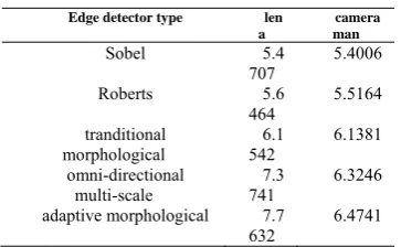
TABLEI
PSNR OF DIFFERENT EDGE DETECTORS (DB)
Edge detector type len a
camera man
Sobel 5.4 707
5.4006
Roberts 5.6 464
5.5164
tranditional morphological
6.1 542
6.1381
omni-directional multi-scale
7.3 741
6.3246
adaptive morphological 7.7 632
6.4741
In the formula above, M×N defined as the size of
image, W i j
( )
, ,W' ,( )
i j separately represent gray valueof source image and segmented-image at position
( )
i j, .In order to show the superiority of the improved algorithm further, the author selected 30 gray images and work out the corresponding PSNR value of 5 kinds edge detection algorithms respectively with the help of MATLAB simulation, the curves were showed as follows:
0 5 10 15 20 25 30
0 3 6 9 12 15
edge maps
P
S
NR(d
B
)
Sobel Roberts tranditional morphological all-dimensional multi-scale adaptive morphological adaptive morphological
Figure 4. Curves of difference algorithm
Where, the curves from top to bottom correspond to the PSNR value connecting line of adaptive morphological algorithm, omni-directional multi-scale algorithm, traditional morphological algorithm, Robert’s algorithm and Sobel algorithm. We can straightforward see that the adaptive morphological algorithm makes the best performance.
VIII.CONCLUSION
Based on the research of basic mathematical morphological operators, the author proposed a new algorithm to restrain noise, which is edge detection based on omni-directional and multi-scale mathematical morphology. Four operations of mathematical morphology (dilation, corrosion, opening operation and closing operation) and the combination of them are adopted. Meanwhile, according to the types and scales of different structural elements, complete image edge information can be detected effectively, and smoothness of the edge can be well maintained. The experimental results show that the improved algorithm can extract edge information effectively and accurately than the single-scale structural element morphological edge detection operator and differential operators such as Sobel operator, Prewitt operator and so on. In the future research, on the basic of extracting abundant edge information and accurate positioning, the author will devote to seeking a real-time algorithm, as far as possible to reduce the algorithm complexity, in order to achieve better edge detection effect.
IX. ACKNOWLEDGEMENT
This project is supported by the National Natural Science Foundation of China(61271305) and the Fundamental Research Funds for the Central Universities(2013JBM009).
REFERENCES
[1] J. Peng, P. Rusch, and T. Herrmann, “Morphological filters and edge detection application to medical imaging,” Proceedings of the Annual Conference on Engineering in Medicine and Biology, v 13, npt1, , 1991,pp. 251-252. [2] Yanfeng Fan, Gangcui Fei, “Application of edge detection
Human-Machine Systems and Cybernetics, pp. 304-307. [3] Lixia Jiang, Wenjun Zhou, Yu Wang “Study on improved
algorithm for image edge detection,” 2010 The 2nd International Conference on Computer and Automation Engineering (ICCAE) pp. 476-479.
[4] M. Sharifi , M. Fathy, M.T. Mahmoudi, “A classified and comparative study of edge detection algorithms,” Information Technology: Coding and Computing, 2002. Proceedings. International Conference on Digital Object Identifier, pp. 117-120.
[5] J. Serra, “Image Analysis Using Mathematical Morphology,” Academic Press, London, 1987.
[6] P. Maragos, “Pattern spectrum and multi-scale shape representation,” IEEE Trans. Pattern Anal. Mach. Intell. 11 (7) (July 1989) pp.701-716.
[7] Dawei Qi, Fan Guo, “Medical Image Edge Detection Based on Omni-directional Multi-Scale Structure Element of Mathematical Morphology,” Automation and Logistics, 2007 IEEE International Conference on Digital Object, pp.2281 – 2286.
[8] Ender Konukoğlu et al, “Shape-based hand recognition”, IEEE Trans Image Process, 2006 Jul;15(7),pp1803-15. [9] Tao Wang, Na Wei, “Multi-scale Mathematical
Morphology based Image edge detection,” Intelligent System Design and Engineering Application (ISDEA), 2012 Second International Conference on Digital Object
Identifier: 10.1109/ISdea.2012.674 pp.1060–1062.
[10]Qing Liu, Chengyu Lai, “Edge Detection Based on Mathematical Morphology Theory,” Image Analysis and Signal Processing (IASP), 2011 International Conference on Digital Object Identifier: 10.1109/IASP.2011.6109018, pp. 151-154.
[11]Xiaojin Zhu, Jie Yang, Alex Waibel. Segment hands of arbitrary Color. Fourth IEEE International Conference on Automatic Face and Gesture Recognition, 2000.pp.1531-1540.
[12]L. Keyes and A.C. Winstanley, “Using Moment Invariants for classifying shapes on large-scale maps Computers”, Environment and Urban Systems, v25, 2001, pp.119-130. [13]R.K.Mehra, “On the identification of variances and
adaptive Kalman filtering, “IEEE Transaction on Automatic Control, AC-15, 1970, pp.175-183.
Hang Zhou Born in Shan’xi, 1974. Received his Phd of Information and Signal Processing at Beijing Jiaotong University,Beijing,China, in 2008.