An Improved CNN Structure Model for Image
Classification Recognition
Ming Ye
1, 2, 3, 4, Zhisai Shi
2, Guangyuan Liu
1*1College of Electronic and Information Engineering, Southwest University, Chongqing, China. 2College of Computer and Information Science, Southwest University, Chongqing, China.
3College of Computer Science and Engineering, Sichuan University of Science and Engineering, Sichuan
Zigong, China.
4Informatics Institute, University of Alabama at Birmingham America, Birmingham.
* Corresponding author. Tel.: +8602368252051; email: [email protected] Manuscript submitted September 10, 2018; accepted November 5, 2018. doi: 10.17706/jcp.13.12.1349-1356
Abstract: In recent years there have been many successes of using deep learning for imaging classification recognition. In this work firstly we discuss in details the differences between machine learning and deep learning from the limitations of traditional machine learning, and gives a detail introduction to the advantages of typical deep convolution neural network in image classification. Deeper neural networks are more difficult to train, this paper presents an improving deep learning convolutional neural network (CNN) structure model and gain accuracy from considerably increased depth. We also show that this improving structure model leads to the prediction results are higher than the original deep-learning CNN structure model with training and testing on the published data set.
Key words: Machine-learning, convolutional neural network, image classification, structure model.
1.
Introduction
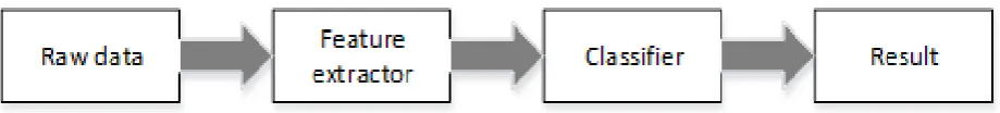
The Convolutional Neural Network (CNN) has shown excellent performance in many computer machine learning problems [1]. Many papers have been published on this topic. Traditional machine learning has a lot of limitations in dealing with image classification issues and raw data. Since the advent of machine learning in the 1980s, the construction of a complete machine learning system requires to experience experts to design feature extractors. The work of these feature extractors is to convert the raw data into appropriate middleware or eigenvectors and then through a variety of classifiers, such as SVM (support vector machine), decision tree, so the input data for the corresponding classification [2]-[4]. However, feature extraction is an important part of the process of data preprocessing. It relies heavily on the construction of feature extractors. The efficiency of the extractor can directly affect the generalization ability of the system [5], [6] (See Fig. 1).
Compared with the machine learning, the depth and structure model of deep learning is more complicated. Of course, the complicated model means that the training efficiency is reduced. However, since the 21st century, with the improvement of computer computing power and the emergence of large data, deep learning is gradually popular [7]- [9].
In the depth of learning, the original data of the data set only need to be simple to provide input for the system, the system structure can automatically build the corresponding feature extractor, without manual participation.
Convolution neural network (CNN) has a good performance in the field of machine vision. It has the following three characteristics of location connections, Weight sharing, and Multi-convolution nuclei compared with the traditional neural network. Its special network structure makes CNN greatly reduce the number of parameters at the same time, but also very good to retain the characteristics of the image [10], [11].
2.
Experiment Methods
To illustrate the superiority of improving CNN in image classification, we used the Caffe deep learning framework, as well as the public data set Cifar10. By improving the CNN structure model, we achieved a good prediction result.
2.1.
Improving Network Structure Model
The improving CNN network structure model selected in the experiment has made some changes in the tail on the basis of the CNN structure model [2], [3]. While the activation function is no longer using the Sig mod function, but the Relu which with the better training result. Furthermore, each convolution layer will be followed by a non-linear processing module. At the same time the structure of the hierarchy is also deeper, adding a sampling layer. In order to better handle the experimental data. A Soft max classifier is added before the output layer to map the vector of the K dimension to the vector of another K dimension so that the value of each vector is in the [0, 1] [12] (See Fig. 2).
Fig. 2. Improving structure model.
2.2.
Data Preprocessing
The experimental data set is cifar-10 data set, the data set a total of 60,000 color pictures, the size of each picture is 32 × 32, of which 50000 training set, test set 10000. The data set is divided into ten categories, the label corresponding to the category from 0-9 followed by airplane, automobile, bird, cat, deer, dog, frog, horse, ship, truck.
2.3.
Normalization
method, the formula is as following:
(1)
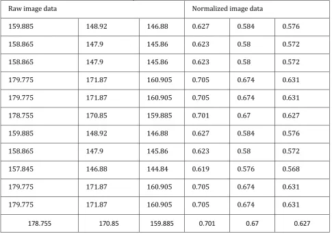
In order to elaborate on this process, we will test the picture (a truck photo) R channel corresponding to the one dimension out of 36 pixels, the process of data changes was visualized (See Table 1).
Table 1. Input Data Normalization Process
Raw image data Normalized image data
159.885 148.92 146.88 0.627 0.584 0.576
158.865 147.9 145.86 0.623 0.58 0.572
158.865 147.9 145.86 0.623 0.58 0.572
179.775 171.87 160.905 0.705 0.674 0.631
179.775 171.87 160.905 0.705 0.674 0.631
178.755 170.85 159.885 0.701 0.67 0.627
159.885 148.92 146.88 0.627 0.584 0.576
158.865 147.9 145.86 0.623 0.58 0.572
157.845 146.88 144.84 0.619 0.576 0.568
179.775 171.87 160.905 0.705 0.674 0.631
179.775 171.87 160.905 0.705 0.674 0.631
178.755 170.85 159.885 0.701 0.67 0.627
2.4.
Subtract the Mean Value
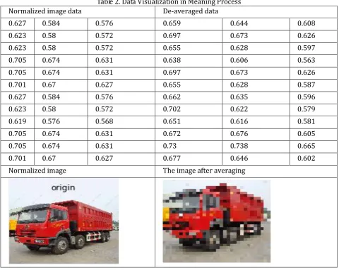
Uncalculating is also a very common method of data processing in image study. The average purpose is to make the whole network speeding up the convergence process in the training process. In this emulation, we take the average of the three channel data of all the pictures in the test data set, and then subtract the average data from the data of the current test picture [15]. The formula is as following (to R channel as an example):
(2)
c
: The size of the data setir
x
: The sum of all R channel valuesWe still have this 36 pixel normalized data and de-averaged data to do a visual comparison of the
255
minmax
min
x
x
x
x
x
x
n
c
x
x
x
c
i
ir
n mr
demonstration (See Table 2):
Table 2. Data Visualization in Meaning Process Normalized image data De-averaged data
0.627 0.584 0.576 0.659 0.644 0.608 0.623 0.58 0.572 0.697 0.673 0.626 0.623 0.58 0.572 0.655 0.628 0.597 0.705 0.674 0.631 0.638 0.606 0.563 0.705 0.674 0.631 0.697 0.673 0.626 0.701 0.67 0.627 0.655 0.628 0.587 0.627 0.584 0.576 0.662 0.635 0.596 0.623 0.58 0.572 0.702 0.622 0.579 0.619 0.576 0.568 0.651 0.616 0.581 0.705 0.674 0.631 0.672 0.676 0.605 0.705 0.674 0.631 0.73 0.738 0.665 0.701 0.67 0.627 0.677 0.646 0.602 Normalized image The image after averaging
From the Table 2 we can see that the mean operation is essentially a micro-processing of data, and we can still recognize the image after visualization.
2.5.
Convolution Process
The training network structure model has a national weight, that is, a fixed eigenvalue. We have taken a weight of the R channel and made a visual demonstration, which helps us to better understand and adjust the convolution neural network (See Table 3).
Table 3. Weight Associated with the First Convolution Layer Weight visualization Weight parameter
0.612 0.621 0.579 0.576 0.587 0.632 0.6 0.571 0.58 0.606 0.614 0.561 0.539 0.56 0.571
0.608 0.569 0.545 0.564 0.572
It can be seen that each convolution kernel represents the characteristics of a part of the input image, some weights are responsible for extracting the gray features, and some weights are extracted from the color features (see Table 3). The feature extraction process is done automatically during the training process of the network, No human intervention. But it has one of the biggest shortcoming is not visible, that is, we cannot know the network training "good" or "bad", through the weight of visualization can indirectly help us to determine the network training effect. Because well-training network weights are usually presented as beautiful, smooth filters; conversely, if the performance of noise filtering, it means that the network has not been enough time to train, or in the training process appeared over the fitting phenomenon. From the Table 3, we can see that this experiment with the first convolution layer connection weight is very beautiful, smooth, indicating that the result of network training is good.
The convolution process is the output of the upper layer, and the convolution kernel carries on the convolution operation, and carries on the nonlinear transformation to obtain the characteristic map of the next layer.
Here we can clearly see the outline of the original image, shape, which is compared with the following convolution layer. Neural network in the construction of feature mapping is a way that we cannot understand.
2.6.
Down Sampling Process
This experiment uses the maximum pool sampling method, the filter size is 2 × 2, the adjacent four values for the polymerization statistics, which not only reduces the number of parameters, but also very good to retain the characteristics of the image (See Table 4).
Table 4. Visualization of Sample Layer Data
Visualization of sample layer data Sample layer data
0.501 0.532 0.57
0.54 0.528 0.555
0.502 0.534 0.555
After the first sampling layer found that the feature mapping layer after sampling, itself has not changed a lot and be able to retain the characteristics of the convolution layer, which on the other hand that the network training effect is well, the network structure is also very reasonable.
2.7.
Convolution - Sampling Alternate Process
Fig. 3. High-level feature mapping layer visualization.
3.
Results
As mentioned above, the purpose of the Soft max classification is to make the results of the experiment mapped to the [0,1] interval, which facilitates the statistics of the data. Soft max is calculated as following:
(3)
The result of Soft max corresponds to the input mapping corresponding to a tag probability. According to higher mathematics knowledge, it is not difficult to draw that this function is actually a monotonically increasing function. That is, the larger input value, the greater the output, the greater probability that the input image belongs to the tag.
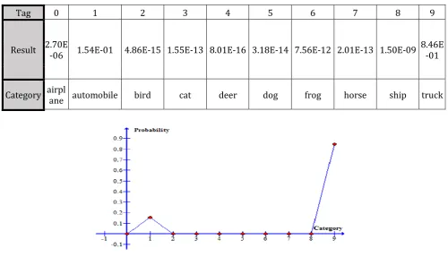
In this experiment, we took a picture of a truck (not a test set), through the convolution of the neural network model and conducted a forward transmission, get the output as following (See Table 5):
Table 5. Result of Classification
Fig. 4. Result of classification a single image.
Tag 0 1 2 3 4 5 6 7 8 9
Result 2.70E-06 1.54E-01 4.86E-15 1.55E-13 8.01E-16 3.18E-14 7.56E-12 2.01E-13 1.50E-09 8.46E-01
Category airplane automobile bird cat deer dog frog horse ship truck
) exp(
) exp( )
max(
j i i
a a a
In order to test the generalization performance of the network, this experiment deliberately selected two similar categories of truck and car. From the results we can see that the network structure that probability of the truck is the largest which up to 83%. The probability of the car is only 16%. The forecast results also meet our basic expectations (See Fig. 4).
4.
Conclusion
The applications of convolution neural network is very extensive, from the traditional face recognition, target detection to the recent very hot art style image migration, are convolution neural network specific application cases.
Although in this experiment, the forecast results were a great success, but there are still a lot of work worthy of our further study. Firstly, in view of the fact that convolution neural networks are getting deeper and deeper, they need large-scale data sets and strong computing power to train. At the same time, in order to further accelerate the training process, GPU training and even TPU training began to gradually toward our vision, but for the general study, the more efficient and more rapid training is still worth pursuing. During the training time, these depth models are demanding on the memory and consume time, which make them unable to deploy on the mobile platform. How to reduce complexity and get a fast executing model without reducing accuracy is an important research direction.
Secondly, a major obstacle to the use of convolution neural networks in the new task is: how to choose the appropriate parameters, such as learning rate, training scale, convolution kernel size, layer number, etc., which requires a lot of technology and experience. These hyper parameters have internal dependencies, which make adjustments very expensive.
Finally, on the convolution neural network, there is still a lack of unified theoretical support. The current convolution neural network model is still a black box, more in-depth understanding of the working principle of the neural network for us to apply this technology better in real life has a vital significance.
Acknowledgment
The work was conducted in the Chongqing Medical University. We thank Dr. Xu Lei for support in data acquisition.
References
[1] Ye, M., Yang, T., Qing, P., Lei, X., Qiu, J., & Liu, G. (2015). Changes of functional brain networks in major depressive disorder: A graph theoretical analysis of resting-state fMRI. PLoS One.
[2] Saha, A., Harowicz, M. R., Wang, W., & Mazurowski, M. A. (2018). A study of association of Oncotype DX recurrence score with DCE-MRI characteristics using multivariate machine learning models. J Cancer Res Clin Oncol.
[3] Zheng, X., Wang, Y., Wang, G., & Liu, J. (2018). Fast and robust segmentation of white blood cell images by self-supervised learning. Micron, 107, 55-71.
[4] Shimoda, A., Ichikawa, D., & Oyama, H. (2018). Prediction models to identify individuals at risk of metabolic syndrome who are unlikely to participate in a health intervention program. Int J Med Inform. 111, 90-99.
[5] Mannil, M., Von, S. J., Manka, R., & Alkadhi, H. (2018). Texture analysis and machine learning for detecting myocardial infarction in Noncontrast low-dose computed tomography: Unveiling the invisible. Invest Radiol.
[7] Delahanty, R. J., Kaufman, D., & Jones, S. S. (2018). Development and evaluation of an automated machine learning algorithm for in-hospital mortality risk adjustment among critical care patients. Crit Care Med.
[8] Mohammed, A., Biegert, G., Adamec, J., & Helikar, T. (2017). Cancer discover: An integrative pipeline for cancer biomarker and cancer class prediction from high-throughput sequencing data. Oncotarget, 9(2),
2565-2573.
[9] Sepehrband, F., Lynch, K. M., Cabeen, R. P., Gonzalez-Zacarias, C., & Zhao, L., D'Arcy, M., Kesselman, C., Herting, M. M., Dinov, I., Toga, A. W., & Clark, K. A. (2018). Neuroanatomical morphometric characterization of sex differences in youth using statistical learning. Neuroimage, 172, 217-227. [10]Usman, S. M., Usman, M., & Fong, S. (2017). Epileptic seizures prediction using machine learning
methods. Comput Math Methods Med, 9074759.
[11]Mutasa, S., Chang, P. D., Ruzal-Shapiro, C., & Ayyala, R. (2018). MABAL: A novel deep-learning architecture for machine-assisted bone age labeling. J Digit Imaging.
[12]Dwyer, D. B., Falkai, P., & Koutsouleris, N. (2018). Machine learning approaches for clinical psychology and psychiatry. Annu Rev Clin Psychol.
[13]Giger, M. L. (2017). Machine learning in medical imaging. J Am Coll Radiol.
[14]Kim, T., Kim, J. W., & Lee, K. (2018). Detection of sleep disordered breathing severity using acoustic biomarker and machine learning techniques. Biomed Eng Online, 17(1), 16.
[15]Ye, M., Qing, P., Zhang, K., & Liu, G. (2016). Altered network efficiency in major depressive disorder.
BMC Psychiatry, 16(1), 450.
Ming Ye was born in China in 1974. He received the B.E, M.E and Ph.D degrees from University of Electronic Science and Technology, Chengdu, China, in 1996, 2005, and 2016, respectively. He joined Southwest University, Chongqing, China, in 2005. Since 2005 he has been with Southwest University, where he is currently an associate professor. His main areas of research interest are artificial intelligence, bioinformatics, machines learning, and big data. Dr. Ye is a member of the Institute of Computer and Electrical Engineers of China. Since October, 2017, he is visiting scholar at University of Alabama at Birmingham.
Zhisai Shi was born in China in 1993. He received the MS degrees from Southwest, Chongqing, China, in 2018, His main areas of research interest are artificial intelligence, bioinformatics, machines learning, and big data. Mr. Shi is a member of the Institute of Computer and Electrical Engineers of China.
Guangyuan Liu was born in China in 1963. He received the B.E, M.E, and Ph.D degrees from University of Electronic Science and Technology, Chengdu, China, in 1982, 1998, and 2002, respectively. He joined Southwest University, Chongqing, China, in 1982. Since 2005 he has been with Southwest University, where he is currently a professor. His main areas of research interest are artificial intelligence, feeling computing, machines learning, and big data. Dr. Ye is a member of the Institute of Computer and Electrical Engineers of China.