ISSN (e): 2250-3021, ISSN (p): 2278-8719
Vol. 09, Issue 6 (June. 2019), ||S (II) || PP 54-63
Model Development for Oxygen Diffusion through Petroleum
Contaminated Soils.
Umeda, Uchendu, and Ehirim,Emmanuel
Department of Chemical/ Petrochemical EngineeringRivers State University, Portharcourt, Nigeria. Corresponding Author:Umeda, Uchendu
ABSTRACT: The aim of this study was to develop a Mathematical model that will predict oxygen concentration at 100cm depth, obtained from oxygen diffusion for bioremediation of petroleum contaminated soils at above mentioned depth. A mathematical model in two dimensional flow(x and z) was developed from basic conservative principle and it was solvednumerically to obtain the final solution. MATLAB 8.1a version (R 2013) was used to simulate the entire process. Results obtained from the model for oxygen concentration at 100cm depth followed the same trend with the experimental results. The results from the model were compared with experimental results and both showed a good fit. Therefore, the developed model can be used for the prediction of Oxygen concentration for bioremediation of petroleum contaminated soils at 100cm depth.
Keyword:
Mathematical Model; Oxygen Diffusion and--- --- Date of Submission: 02-06-2019 Date of acceptance: 17-06-2019 --- ---
I.
INTRODUCTION
Bioremediation is a process that offers the possibilities to destroy or render various contaminants harmless, using natural biological activities (Vidali, 2001). Bioremediation involves three principal approaches namely, natural attenuation, bio-stimulation and bio-augumentation (Chikere et al., 2009a). For effectivebioremediation to take place in the soil, there must be sufficient soil nutrient and oxygen concentration, to enhance the activities of microorganism (Umeda et al., 2017). Nutrients are easily assimilated by soil microorganisms in soil pollution with crude oil, thus reducing the nutrient reserves (Rahman et al., 2002). Petroleum biodegradation is highly dependent on environmental conditions and on the chemical structure of the pollutant compounds (Swannell et al., 1996; Aldrett et al.,1997). The rates of degradation and the quality of hydrocarbon eliminated also depend on the type and amount of hydrocarbon present at the contaminant site (Del Arco and de Franca, 2001). Components that are low in molecular weight such as the aliphatic hydrocarbons tend to be degraded first, leaving behind the much larger molecules (aromatic hydrocarbon) which take much longer to break down. The lighter carbon components of the crude oil are also less viscous and can easily degrade and become volatile when acted upon by weather and environmental elements. This trend indicates the presence of biodegradation by microbial bacteria who cannot break down the larger oil compounds left after the initial phases of degradation (Ezra et al., 2000). Hydrocarbons from crude oil are substrates for microorganisms, hence, when an accidental oil spill occurs, the number of hydrocarbon degrading microorganisms in the ecosystem increases. The speed and efficiency of bioremediation of a soil contaminated with petroleum and petroleum products depend on the number of hydrocarbon-degrading microorganisms in the soil. The most important factors for population growth are temperature, oxygen, pH, content of nitrogen and phosphorus, hydrocarbon class and their effective concentration. Also, the degree and rate of biodegradation are influenced by the type of soil in which the process occurs (Van hmm et al., 2003).
DEVELOPMENT OF MATHEMATICAL MODEL
Figure 1. Schematic Diagram for the Hypothetical Control Volume Representation of Soil Sample
Considering the conservation of species A, including production of A by chemical reaction within the volume. The general relation for mass balance of species A for the control volume is stated as
0
volume
control
the
A within
of
production
chemical
of
Rate
volume
control
within
A
of
on
Accelerati
of
rate
Net
volume
control
from
A
of
efflux
mass
of
rate
Net
(1)
Defining individual terms in equation (1) and deriving from basic conservative principle, we obtain the following.
The net rate of mass efflux from the control volume could be evaluated by considering the mass transferred across control surfaces. Hence, the mass of A transferred across the area
∆y∆z at xwill be
AV
Ax
y
z
/
x
That is,
n
Ax
y
z
/
x
.The net rate of mass efflux of component A will be In the x-direction:
n
Ax
y
z
/
xx
n
Ax
y
z
/
xIn the y – direction:
n
Ay
y
z
/
y
y
n
Ay
y
z
/
y
and in the z – direction: nAzxy/zznAzxy/z Rate of accumulation of volume A with control =x
y
z
t
A
Rate of reaction by chemical reaction = rAxyz Substituting each terms in equation (1), we obtain
y
z
x
x
n
y
z
x
n
x
z
y
y
n
x
z
y
n
x
y
z
z
n
x
y
z
n
Ax/
Ax/
Ay/
Ay/
Az/
Az/
0
z
y
x
z
y
x
t
AA
(2)
Dividing through by the volumexyz, and cancelling terms, we have
0
A A Az
AZ Ay
Ay Ax
AX
t
z
z
n
z
z
n
y
y
n
y
y
n
x
x
n
x
x
(3)
0
A A Az Ay Axr
t
z
y
x
(4)Eq. (4) is the equation of continuity of component A. As
Ax,
Ay and
Az are the rectangular componentsof the mass flux vector,
Ax; equation (4) may be written0
A AA
r
t
n
(5)A similar equating continuity for component B in the same manner. The differential equation are
0
B B Bz By Bxr
t
z
n
y
n
x
n
(6)and
.
0
B BB
r
t
n
(7)Adding equations (5) and (7), we obtain:
0
.
A B A BB
A
r
r
t
n
n
(8)But ρV V ρ V ρ η
ηA B A A B B
B AV
ρ =
ρ
Substituting these relation with eq. (8)
r
r
0
t
ρ
.ρρ
A
B
(9)Eq. (9) represents the continuity equation for the mixture. Writing equation (9) in substantial derivative
0
.V
ρ
Dt
Dρ
0
.
A AA
r
Dt
DW
(10)
Molar equivalent of eq. (5) and (7) are For component A
0
A AA
R
t
C
N
(11)For component B
0
B BB
R
t
C
N
(12)and for mixture (adding equation (11) and (12)) we have
0
A B A BB
A
R
R
t
C
C
N
N
(13) For a binary mixtureCV V C V C N
NA B A A B B
and CACB C
A B, RA = -RB
0
)
(
.
R
AR
Bt
C
CV
(14)Recall,
A B
A A rB
A CD y y N N
N .
= A
A B
z A y A x A
AB
y
N
N
y
y
y
CD
V C y CD
NA AB A A (15)
Substituting eq. (15) into eq. (11), we obtain
0
.
.
A AA A AB
R
dt
C
V
C
y
CD
(16)0
2
A AA A AB
R
t
C
V
C
y
CD
Eq. (16) describes concentration problems within a diffusing system. This equation is relatively unwieldy. These equations can be simplified by making restrictive assumptions.
Assumptions:
1. If the density
ρ
and DAB are constant0
2
A AA A AB
R
t
C
C
V
y
CD
0
.
2
A AA A AB
R
t
C
C
V
C
D
0
.
.
2
A AA A A AB
r
t
V
V
D
Dividing each term by the molar weight of component A and rearranging we obtain
A A AB A
A
D
C
R
t
C
C
V
2.
(17)R
z
C
y
C
x
C
D
t
C
z
C
V
y
C
V
x
C
V
A A AAB A A z A y A x
2 2 2 2 2 2 (18) WhereThe solution to equation (18) was solved numerically
using the Finite Different Approximation (FDA) in the explicit scheme. Thus, resolving the resulting partial differential equation numerically, we obtain the following:
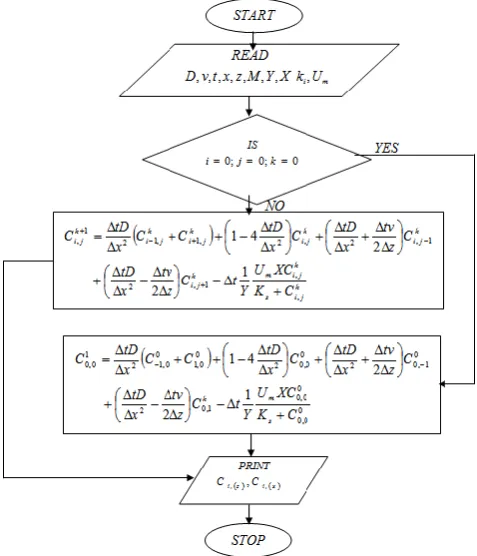
The initial and boundary conditions are as follows At t = 0, 𝑧 ≥ 0 𝑎𝑛𝑑 𝑥 ≥ 0: 𝐶 = 0
At t > 0, 𝑧 = 0 𝑎𝑛𝑑 𝑥 = 0: 𝐶 = 𝐶0
At t> 0, 𝑧 > 0 𝑎𝑛𝑑 𝑥 > 0: 𝐶 = 𝐶∞
t
C
C
t
C
ikj k j i
, 1 , (19)z
C
C
z
C
ikj k j i
2
1 , 1 , (20) 2 , 1 , , 1 2 22
x
C
C
C
x
C
ik jk j i k j i
(21) 2 , 1 , , 1 2 22
y
C
C
C
y
C
ik jk j i k j i
(22) 2 1 , , 1 , 2 22
z
C
C
C
z
C
ikjk j i k j i
(23)The diffusion of oxygen in y direction is minimal because of the driving force in the z direction, so the diffusion of oxygen in the y direction is insignificant.
Substituting equations (19) and (23) into (18) yields:
S
K
SX
Y
R
s m
k j i k j i k j i k j i k i k j i k j i k j i k j i k j i k j i
R
z
C
C
v
z
C
C
C
x
C
C
C
D
t
C
C
, 1 , 1 , 2 1 , 1 , 2 , 1 , , 1 , 1 ,2
2
2
(24)For uniform grids
x
z
, therefore, equation (6) becomes
kj i k j i k j i k j i k i k j i k j i k j i k j i k j i k j
i
C
C
tR
z
tv
C
C
C
C
C
C
x
tD
C
C
1 , 2 1, , 1, , 1 , 1 , 1 , 1 ,,
2
2
2
(25)Collection of like terms
kj i k j i k j i k j i k j i k j i k j
i
C
tR
z
tv
x
tD
C
z
tv
x
tD
C
x
tD
C
C
x
tD
C
, 1 2 1, 1, 2 , 2 , 1 2 , 1 ,2
2
4
1
(26)Also, the reaction term
S
K
SX
U
Y
R
s m k ji
1
, and
S
C
.Hence, k
j i s k j i m k j i
C
K
XC
U
Y
R
, , ,1
(27)Substituting equation (7) into (6) gives
k j i s k j i m k j i k j i k j i k j i k j i k j iC
K
XC
U
Y
t
C
z
tv
x
tD
C
z
tv
x
tD
C
x
tD
C
C
x
tD
C
, , 1 , 2 1 , 2 , 2 , 1 , 1 2 1 ,1
2
2
4
1
(28)Equation (28) is the numerical solution in two dimensional flow (x and z) to the model in the explicit scheme. Where C- Initial Oxygen Concentration, D-Diffusion coefficient of oxygen in the soil, Y- Yield conversion constant, Um - Maximum specific growth rate, KS – Substrate Saturation constant, Z- Distance, t – Time.
Equation (28) is the model for prediction of oxygen concentration with time and depth along the reactor.
Calculation Algorithm
II.
RESULTS AND DISCUSSION
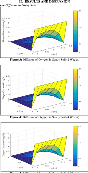
Surface Plot of Oxygen Diffusion in Sandy Soils
Figure 3: Diffusion of Oxygen in Sandy Soil (2 Weeks)
Figure 4: Diffusion of Oxygen in Sandy Soil (4 Weeks)
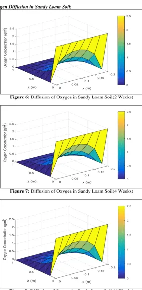
Surface Plot of Oxygen Diffusion in Sandy Loam Soils
Figure 6: Diffusion of Oxygen in Sandy Loam Soil(2 Weeks)
Figure 7: Diffusion of Oxygen in Sandy Loam Soil(4 Weeks)
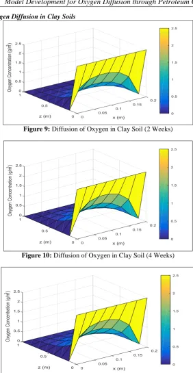
Surface Plot of Oxygen Diffusion in Clay Soils
Figure 9: Diffusion of Oxygen in Clay Soil (2 Weeks)
Figure 10: Diffusion of Oxygen in Clay Soil (4 Weeks)
Figure 11: Diffusion of Oxygen in Clay Soil (6 Weeks)
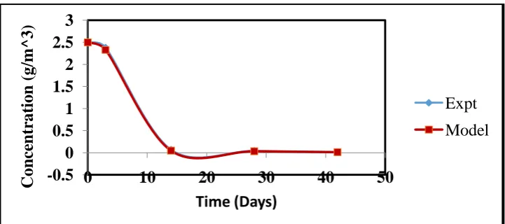
COMPARISON BETWEEN EXPERIMENTAL AND MODEL PREDICTIVE DATA FOR OXYGENCONCENTRATION.
The basis of the comparison of the experimental and model data was to show the fitness of the data at all data point and the trend obtained from the experimental and predictive model results.
Figure 12: Comparison between Experimental and Model Predictive Data for Sandy Soil
Figure 13: Comparison between Experimental and Model Predictive Data for Sandy Loam Soil
Figure 14: Comparison between Experimental and Model Predictive Data for Clay Soil
Figures 12- 14, indicated that the predictive model gives very good fit of experimental Data at all Data point with an error of 0.01%, 0.04% and 0.02% for Sandy Soils, Sandy Loam Soil and Clay Soil respectively. Also, it showed that the results of the experimental and predictive model followed the same trend.
-0.5
0
0.5
1
1.5
2
2.5
3
0
10
20
30
40
50
Conce
n
tr
at
ion
(
g/m
^3)
Time (Days)
Expt
Model
-0.5
0
0.5
1
1.5
2
2.5
3
0
10
20
30
40
50
Conce
n
tr
at
ion
(
g/m
^3)
Time (Days)
Expt.
Model
-0.5
0
0.5
1
1.5
2
2.5
3
0
10
20
30
40
50
Conce
n
tr
at
ion
(
g/m
^3)
Time (Days)
Expt
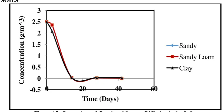
COMPARISON OF OXYGEN DIFFUSION IN SANDY SOILS, SANDY LOAM AND CLAY SOILS
Figure 15: Comparison of Results of Oxygen Diffusion in the Soils.
Figure 15 shows the graph of oxygen diffusion in Sandy soils, Sandy loam and Clay soils. Comparison of Oxygen diffusion in Sandy soils, Sandy loam and Clay soil reveal that the diffusion of Oxygen is highly appreciable in Clay Soil compared to Sandy and Sandy loam soils. This may be as a result of the particle size of the soils, surface area, and porosity of the soils.
III.
CONCLUSION
In line with the results obtained from this study, it is important to state that the developed mathematical model can be used for the prediction of Oxygen concentration for bioremediation of petroleum contaminated soils at 100cm depth.
REFERENCES
[1]. Aldrett, I., Bonner, S., Mills, J.S., Antenneth, M.A. & Stephen, R.L.(1997). Microbial degradation of crude oil in Marine environments tested in ask experiment. Water Research, 31,2840-2848
[2]. Chikere, C.B., Okpokwasili G.C., & Ichiakkor, O. (2009a). Characterisation of hydrocarbon utilizing bacteria in tropical marine sediments. African Journal of Biotechnology, 11,2541-2544
[3]. Del Arco, J.P. & De Franca, F.P. (2001). Influence of oil contamination level on hydrocarbon biodegradation in sandy sediment. Environmental Pollution, 110, 515-519
[4]. Ezra, S., Feinstein, S., Pelly, I., Banman, D. & Miloslavsky, I. (2000).Weathering of fuel oil spill on the east Mediterranean coast, Ashdod, Isreal.Organic Geochemistry.3, 1733-1741.
[5]. Rahman, K.S.M., Thahira-Rahman, J., Lakshamapernmalsamy, P.& Banat, I. M. (2002).Towards efficient crude oil degradation by a mixed bacterial consortium.Bio-resources Technology, 85, 257 – 261. [6]. Swannel, R.P.J.,Lee, K. & Mc Donagh, M. (1996). Field evaluation of marine oil spill bioremediation.
Microbiological Review, 60, 343-365.
[7]. Umeda, U., Puyate, Y.T., Dagde, K.K. & Ehirim, E.O. (2017). Effect of oxygen diffusion on Total Petroleum Hydrocarbon in Petroleum contaminated soils. International Journal of Engineering and Modern Technology,3. 18-24
[8]. Van Hamme, J.D., Singh, A. & Ward, O.P. (2003). Recent advances in petroleum microbiology. Microbial Molecular Biology Review, 67, 503-549.
[9]. Valadi, M. (2001). Bioremediation. An overview, Appli. Chem, 73, 1163 -1172