Locating Software Faults Based on Control Flow
and Data Dependence
Chenghui Hu
Lab of Intelligent Computing and Software Engineering Zhejiang Sci-Tech University Hangzhou Zhejiang, 310018, China
Email: [email protected]
Zuohua Ding
Lab of Intelligent Computing and Software Engineering Zhejiang Sci-Tech University Hangzhou Zhejiang, 310018, China
Email: [email protected]
Abstract—Debugging software is a difficult and time-consuming work. Fault localization techniques are becoming extremely important. Coverage Based Fault Localization (CBFL) is very commonly used in fault location technique. Tarantula is a typical one. It uses the coverage statistics of failed execution paths and passed execution paths to calculate the suspiciousness in the software. However, since this technique ignores the data dependency, it is hard to find the bugs which are not in the suspicious code area but have data dependence with it. In order to improve the efficiency of fault locating, we combine control flow coverage information and data dependence from program slicing. We validate our approach experimentally using Siemens benchmark programs. The experimental results show that our approach is more effective than Tarantula.
Index Terms—Fault location, Control flow, Program slicing,Data dependence
I. INTRODUCTION
As the scope and complexity of software become increasingly tremendous, it is an increasingly challenging task to locate software faults. Debugging is the main method to locate fault in software, however, it is time-consuming [1]. At present program slicing and program spectrum-based methods are currently the main fault location techniques. Mark Weiser recommended program slicing of error variable to exclude uncorrelated statements [2]. Program slicing is a well-known analysis technique that extracts all statements that affect variables of interest in the program [3][4][5][6]. An execution slice-based technique as reported in [7] can be effective in locating the faults. Coverage based fault location (CBFL) techniques [8][9][10][11][12] (such as Tarantula, SBI) have been used to support software debugging, these methods use well designed test cases to get the program coverage information, then the program spectra of passed and failed executions [13] is contrasted to calculate the suspiciousness [9] of individual program
entities. Finally, software developers check the program entities according to the statements ranking in terms of their fault suspiciousness. However, there are still some cases such as available approaches make unsatisfactory results, because the coverage statistics of program entities are calculated separately. Several studies [14][15] have put forward that such calculation ignores the propagation of infected program states among them , which may cause that located entity is not the really fault. Lei Zhao proposed a context-aware fault localization approach FP via control flow analysis [14]. Eric Wong proposed a novel approach using execution slices and inter-block data dependence to effectively locate the faults to overcome these problems [16].
In order to further improve the efficiency of fault location and decrease the rate of code inspection, we combine control flow edge coverage with data dependence based slice technique, and calculate the control flow edge suspiciousness, then rank the basic blocks in descending order of their suspiciousness. Although the bug may not be in the suspicious code area, it is likely to have relationships with those codes that have data dependence with the suspicious code area. We continue to use the data dependence to locate the fault. Finally, we conduct experiments to validate the effectiveness of our approach using benchmarks. The experiment results show that our method is more effective in locating a program bug by examining less code before finding the really faulty statement than the CBFL technique Tarantula in general.
The paper is organized as follows: In Section II we introduce a simple example with Tarantula technique. Section III discusses our method. In Section IV, we evaluate our method with experiments. Section V concludes the paper and discusses the future work.
II. AN EXAMPLE
as we can see from the Fig. 1. According to past studies [2][10][17][18][19], first, we use some designed test cases to run the program and get the information whether the program will pass the test or not. We also get the coverage information of the program code lines, if a statement is covered by a test case, we will record the statement as 1, conversely record it as 0. If a statement is covered by more failed test cases, the statement is more likely to contain the fault. Next, we calculate the suspiciousness of each statement, the formula is as below:
( ) ( )
( ) ( )
failed s totalfailed suspiciousness s
passed s failed s totalpassed totalfailed
The passed(s) represents the number of succeed test cases cover the statement s; failed(s) represents the number of failed test cases cover the statements; totalfailed represents the number of failed test cases; totalpassed represents the number of succeed test cases.
Then we rank them in descending order and examine the statement until the fault is found. Finally we get the percentage of code inspection; the result is about 13.3%. Next, we recommend our method though this example in the next section.
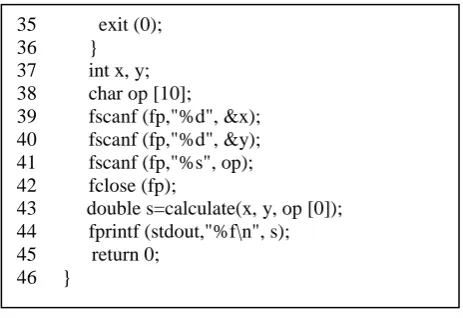
Figure 1: The source code of program
III. METHODLOGY
In this section, we introduce the basic definitions and related techniques firstly, and then explain our method. Besides, we also take the above example described in Fig. 1 to illustrate the procedure of our method and compare the efficiency of fault location.
A. The Fault Location Based on Control Flow Edge
We first introduce some definitions, A Control Flow Graph (CFG) is an execution graph G = (B, E), B = {b1,
b2 … bm} represents the basic blocks, which are
consecutive statements or expressions containing no transfer of control except at the end. E = {e1, e2… ek}
represents the control flow edges that go from one block to the other. Besides, we define Path = {p1, p2… pn}, e (bi,
bj) represents the edge that goes from block bi to bj, e(*, bj)
represents all the edges that go to bj and e (bi,*)
represents all the edges that start from bi.
B. The Fault Location Based on Program Slicing Technique
Program slicing technique is used for decomposition of a program [20]. It is one of fault location methods originally proposed by Mark Weiser [21]. A slice contains a set of statements that might influence the value of a variable v at point s, which is based on dependence analysis. Data dependence means that a variable is depended on another statement, or vice versa.
C. Caculate the Suspiciousness of the Basic Block
1) The theory and method
We recommend the fault location technique based on control flow edge [14] according to a simple example. 1 # include <stdio.h>
2 double add (int x, int y) {
3 double s=0;
4 if(x>0 && y>0) {
5 s=x+y;
6 }
7 return 2*s;//正确为return s; 8 }
9 double sub (int x, int y) {
10 double s=0;
11 if(x-y>0) { 12 s=x-y;
13 }
14 return s; 15 }
16 double calculate (int x, int y, char op) 17 {
18 double s=0;
19 switch (op) {
20 case '+': s=add(x, y); break; 21 case '-': s=sub(x, y); break; 22 }
23 return s; 24 }
25 int main (int argc, char *args []) {
26 FILE *fp;
27 if (args [1] ==NULL) { 28 fp=stdin;
29 }
30 else {
31 fp=fopen (args [1],"r");
32 }
33 if (fp==NULL) {
34 fprintf (stout, "error\n");
35 exit (0);
36 }
37 int x, y; 38 char op [10];
39 fscanf (fp,"%d", &x); 40 fscanf (fp,"%d", &y); 41 fscanf (fp,"%s", op); 42 fclose (fp);
43 double s=calculate(x, y, op [0]); 44 fprintf (stdout,"%f\n", s); 45 return 0;
Figure 2: The program and control flow graph
This basic block is B ={b1,b2,b3,b4,b5}, the control
flow edge is E={e(b1,b2), e(b2,b3), e(b2,b4), e(b3,b5),
e(b4,b5)}, the execution path is Path={b1→b2→b3→b4,
b1→b2→b4→b5}. The formula of edge suspiciousness
calculation is
( )
( ) (1)
( ) ( ) i i i i failed e e
passed e failed e
failed (ei) and passed (ei) respectively represent the
number of failed executions and passed executions that cover ei. In this example, probin(e(s,d)) represents the
proportion of θ(e(s,d)) to θ(e(*,d)), that is the start suspiciousness of e(s,d). probout(e(s,d)) represents the
proportion of θ(e(s,d)) to θ(e(s,*)), it represents the destination suspiciousness of e(s,d)
(*, )
(*, )
( ( , ))
( ( , )) (2)
[ ( (*, ))] e d in
e d e s d prob e s d
e d
( ,*) ( ,*) ( ( , ))( ( , )) (3)
[ ( ( ,*))] e s out
e s e s d prob e s d
e s
In this example, we suppose that all the executions that cover e (b3, b5) succeed and those cover e (b4, b5) failed.According to (1), we can calculate the proneness of b4
and b5, which means the probability of a block containing
faults.
4 5 4 4 5
4 5 3 5
2
( ( , ))
( )
( ( , ))
2
( ( , ))
( ( , ))
in
e b b
proness b
prob e b b
e b b
e b b
4 55 4 5
4 5
( ( , ))
( ) ( ( , )) 1
( ( , ))
out
e b b
proness b prob e b b
e b b
According to the fail execution path = {b1,b2…bn}, bi-1
represents the predecessor block of bi, bi+1 represents the
successor block of bi.
1 1 1
( (
, ))
(
) :
( )
( (
, ))
in i i
i i
out i i
prob e b
b
proness b
proness b
prob
e b
b
Next, in this way we can get the ratio of fault proneness of blocks from bi to bn.
1 2
1
1 2 1 1
1
1 2 1 1
( ) : ( ) : ... : ( )
( , ) ( , )
= 1: : ... :
( , ) ( , )
n
i n
out i out i i
i n
in i in i i
proness b proness b proness b
prob b b prob b b
prob b b prob b b
This ratio of proneness is corresponding to a failed execution, considering the entire program, we add all the fault proneness values which cover the same block, and then the sum of fault proneness represents the block suspiciousness, which is shown in below formula.
( ) ( i( ) | ( i) 0 & & i) suspiciousness b
proness b failed path bpath In fact, the structure of a program is often very complex when the program contains circulations, so the construction of CFG will be more complex. Lei Zhao’s paper didn’t mention this case especially. In our paper, we make the following treatment. 1) If the basic block occurs firstly in the execution, we calculate its suspiciousness. 2) If the basic block doesn’t occur firstly in the execution, we don’t make any changes for the suspiciousness.2) The method implementation
First, we need to record the code coverage information; we use the gcov tool which GNU gcc compiler comes with to acquire the coverage information. Meanwhile we can get the .gcno file which records the basic block and arc information, though which we can construct the control flow graph. Next, we can get the execution path of a test case by the code lines coverage information combining with the code lines the basic block corresponding to. Finally we can calculate the suspiciousness of the basic block.
D. Construct the Program Slice Based on Data Dependence
We get the ranking of the suspiciousness of basic blocks according to the control flow edge coverage information, make use of variable data dependence relation and then choose the block which suspiciousness is the biggest as the slice defined as D(1) . Ef and Ep
respectively represent the code set that failed test cases and the succeed test cases cover, Eall means all code sets.
Next, we examine whether D(1) contains fault or not. If it does, we can locate the fault directly, if it doesn’t contain the fault, we expand the code. W.Eric Wong presents an augmentation method to include additional code [16], in his method, the slice D(1) = Ef - Ep , θ = Ef - D(1), which
means the code area to examine additionally. In our paper, D(1) represents the basic block which suspiciousness is the biggest. Besides, we defined θ = Eall - D(1),
considering more data dependency. We also define the data dependence relation as @, if and only if α defines a variable i used in D(1) or α uses a variable j defined in D(1), that is, a and D(1) have the data dependence relation , which is defined as a@ D(1). The process is introduced as follows:
Step1: Define the slice S (1), which is the first code segment examined, S (1) = {a| a
θ &( a@D(1))}. Step2: Set i = 1.Step3: Examine the S(i) to see whether it contains the fault. Step4: If true, that is, the fault is located in the slice, then
stop. Step5: Set i = i+1.
Step6: Define the slice S(i) = S(i-1)
{a| a
θ &( a@SS(i) is the code segment of the ith iteration.
Step7: If S(i) = S(i -1), that is, no new code segment can be included to the slice, then stop.
Step8: Go back to Step3.
In this process, we utilize the data dependence to construct the S(i), we can see that S(1)
S(2)
S(3)…...By using the method described in the above part, we calculate the suspiciousness of basic block in the Fig. 1. The result is shown in TABLE I.
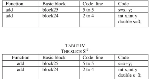
Next, we select the biggest suspiciousness of basic block as the slice D(1) and examine the statements in it, as we can see in the Table II. Although the fault may not be in the suspicious code area, it is likely to have relationships with those codes that have data dependence with it. So if the bug is not in D(1), then we need to examine the additional code in S(1), S(2), etc. Finally, we calculate the percentage of code inspection.
We don’t find the bug by examining the slice D(1), so we expand the code and get the slice S(1) after 1th iteration, as we can see from the Table III. After examining the slice S(1), we don’t find the fault still, so we continue to expand the code . The result is shown in Table IV.
We find the fault in the function add by examining the slice S(2), we locate the fault successfully after examine 5 lines code. We can calculate the percentage of code inspection, which is about 10.87%. By contrast, we use
Tarantula which is the traditional fault location method based on coverage information to get the location effect. From the section II, we can know the percentage of code inspection is about 13.3% with Tarantula. By this simple example, we can see that the effect of our method is better. In order to further validate our method, we conclude a serial of experiments in next section.
IV. THE EXPERIMENTAL EVALUATION
In this section we conduct the experiments to evaluate the effect of our method.
A. Experimental Setup
In this study, we use the Siemens suite [22] as the subject programs, which is the most common test suite used to evaluate the effect of fault localization techniques. An overall description of Siemens suite is presented in Table V. Take the print_tokens for example, it has seven faulty versions, and each of them has exactly one fault. The line of codes are 472, the number of test cases are 4056. There are 132 faulty versions of the seven subject programs in total. We select Tarantula [17] which is a typical CBFL technique to compare with our method. In our experiments, we all select 115 faulty versions to conduct the experiments in accordance with the paper. We only consider the single error in this experiment, so we exclude the version1 of “pint_tokens”, versions2 and 7, version21 of “replace”, version3, 10, 11, 15, 31, 32, 33 and 40 of “tcas”. The errors in version4 and 6 of “print_tokens” occur only in the header files, we also exclude them. Version 10 of “print_tokens2”, version9 of “schedule2” and version 32 of “replace” have no test cases fail, so they are not considered by our experiments. We could collect the coverage information. The experiment environment we use is Ubuntu 12.04 and the TABLE I
THE SUSPICIOUSNESS OF BASIC BLOCK
Function Basic block Code line Suspiciousness
main block1 25,27 0
main block2 28 1
main block3 31 0
main block4 33 0.5
main block5 34 0
main block6 35 0
main block7 39 1
main block8 40 2
main block9 41 4
main block10 42 8
main block11 43 6.4
main block12 44 12.8
main block13 45 25.6
main block14 virtual block 2.5 calculate block15 16,18,19 0 calculate block16 20 80 calculate block17 21 0 calculate block18 23 32 calculate block19 virtual block 0.2
sub block20 9,10,11 0
sub block21 12 0
sub block22 14 0
sub block23 virtual block 0
add block24 2,3,4 80
add block25 5 160
add block26 7 80
add block27 virtual block 1.33
TABLE II THE SLICE D(1)
Function Basic block Code line Code
add block25 5 to 5 s=x+y;
TABLE III THE SLICE S(1)
Function Basic block Code line Code
add block25 5 to 5 s=x+y;
add block24 2 to 4 int x,int y double s=0;
TABLE IV THE SLICE S(2)
Function Basic block Code line Code add block25 5 to 5 s=x+y; add block24 2 to 4 int x,int y
double s=0;
TABLE V
STATICS OF SUBJECT PROGRAMS
Program Faulty Versions Loc Test Cases
print_tokens 7 472 4056
print_tokens2 10 399 4071
replace 32 512 5542
schedule 9 292 2650
schedule2 10 301 2680
tcas 41 141 1578
compiler is gcc4.6.1, we use gcov to collect the coverage information.
B. Evaluation Metric
At present, the evaluation metric of fault location adopted frequently is the score method represented by Jones [17]. In this paper we also use the score as the evaluation metric, which means the percentage of statements have to be examined until the fault is found. First, we calculate the suspiciousness of the basic block and rank them in a descending order. Code with a higher suspiciousness should be examined before that with a lower suspiciousness. The score is defined that (s / S) * 100%, s represents the number of statements we should examine until finding the fault and S represents the number of executable statements. In our experiments, considering that the codes we need to examine contain executed and partial non-executed statements, S represents the size of program.
C . The Result Analysis
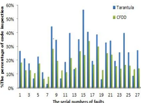
We denote our method based on control flow and data dependence by CFDD. In this experiment, we select the CBFL technique such as Tarantula to compare with our method CFDD. As we can see from the Fig. 3, the x-axis represents the serial numbers of faults, and we select a part of fault numbers which is 115 in total, which reflects the overall condition. The partial fault numbers is shown in the following figure. The y-axis indicates the percentage of code that need to be examined to locate a fault, i.e the percentage of code inspection. If the length of the bar is longer, the corresponding fault location technique is less effective. For example, when the serial numbers of faults is 2, the percentage of code inspection is about 21% with the Tarantula method while our method is about 12.4%, which represents that CFDD is more effective clearly. By the Fig. 3, we can also find that the CFDD does not always perform well for every fault; sometimes the code inspection is a little higher than Tarantula technique.
In order to illustrate the issue, we calculate the average code inspection percentage on the seven programs of the Siemens suite. It is shown in the Table VI. As we can see from the Table VI, CFDD method performs better than Tarantula on most of the seven programs, while the effect of CFDD is lower than Tarantula on two versions. By analyzing the experiment results, we find that when the code inspection percentage is low with Tarantula, our method performs slightly worse than Tarantula. We can also find similar phenomenon mentioned in Lei Zhao’s paper. If fault location is the place where the failures
Figure 3: The comparison of code inspection percentage among Tarantula and our method
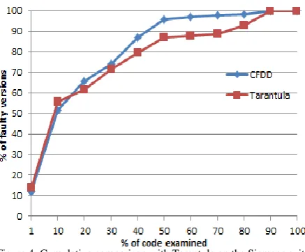
occur, and then the Tarantula is skilful in locating this type of errors. When the code inspection percentage with Tarantula technique is high, our method tends to perform better. Because our method is based on the control flow coverage information, it is good at locating some complex faults that appear in branch condition. Our method is also based on data dependence; it can locate the type of error such as the variable definition and the missing code line. In Fig. 4, we illustrate the cumulative distribution of effectiveness scores per analysis method where the x-axis indicates the percentage of code that needs to be examined. The y-axis represents the percentage of the fault version that fault has been located account for all the fault versions. For example, if the value of horizontal axis is 30, the responding value of y-axis is 71.3, which means if we examine 30% code, we can find the errors of 71.3% fault versions. From the Fig. 4 we can find that although our method does not perform well in all types of faults, our method is very promising in the fault location. When the code inspection percentage is above 15% approximately, our method can examine more faulty versions than Tarantula technique. We consider the past studies, such as the FP method based on control flow analysis, Lei Zhao combines the FP with Tarantula, first uses the Tarantula technique to locate errors, if the error is not found until the percentage of code inspection is up to some value, use the FP instead. The results show that it is more effective clearly.
TABLE VI
THE COMPARISON OF CODE INSPECTION PERCENTAGE BETWEEN
TARANTULA AND OUR METHOD ON THE SIEMENS SUITE
version print _toke ns
print _toke ns2
rep lac e
sched ule
sched ule2
tca s
tot_i nfo
Av era ge
Ta ran tul a
12.6 34.9 12. 4
29.8 36.5 38. 8
41.6
CF D D
14.3 28.6 16. 2
24.3 31.3 24. 5
Figure 4: Cumulative comparison with Tarantula on the Siemens suite
V. CONCLUSIONS AND FUTURE WORK
In this paper, we introduce the fault location technique based on control flow information and data dependency. We use the control flow paths to analyze the program and calculate the block suspiciousness, then we use variable data dependence relation to choose the biggest suspicious block, then increase the search domain to locate the really fault. Finally, we calculate the percentage of code inspection. Experimental results show that our approach could find bugs with lower code inspection by programmers. Our method performs better than the Tarantula.
In the future, we plan to study what effect different types of faults and different test cases have on our fault location method. We are also trying to integrating with Tarantula further and see if we can get better results. Besides, the program in Siemens suite only contains one error, what if the program contains multiple faults; this problem is worthy to study further.
ACKNOWLEDGMENT
This work is supported by NSFC under Grants No. 61210004 and 61170015.
REFERENCES
[1] Jones, James Arthur. Semi-automatic fault localization. Diss. Georgia Institute of Technology, 2008.
[2] Weiser, Mark. "Programmers use slices when debugging." Communications of the ACM 25.7 (1982): 446-452. [3] Agrawal, Hiralal, and Joseph R. Horgan. "Dynamic
program slicing." ACM SIGPLAN Notices 25.6 (1990): 246-256.
[4] Kusumoto, Shinji, et al. "Experimental evaluation of program slicing for fault localization." Empirical Software Engineering 7.1 (2002): 49-76.
[5] Mock, Markus, et al. "Improving program slicing with dynamic points-to data." Proceedings of the 10th ACM SIGSOFT symposium on Foundations of software engineering. ACM, 2002.
[6] Miao, Chunyu. "Dynamic Slicing Research of UML Statechart Specifications." Journal of Computers 6.4 (2011): 792-798.
[7] Agrawal, Hiralal, Richard A. DeMillo, and Eugene H. Spafford. "Debugging with dynamic slicing and
backtracking." Software: Practice and Experience 23.6 (1993): 589-616.
[8] Abreu, Rui, et al. "A practical evaluation of spectrum-based fault localization." Journal of Systems and Software 82.11 (2009): 1780-1792.
[9] Yu, Yanbing, James A. Jones, and Mary Jean Harrold. "An empirical study of the effects of test-suite reduction on fault localization." Proceedings of the 30th international conference on Software engineering. ACM, 2008.
[10]Jones, James A., and Mary Jean Harrold. "Empirical evaluation of the tarantula automatic fault-localization technique." Proceedings of the 20th IEEE/ACM international Conference on Automated software engineering. ACM, 2005.
[11]Chilimbi, Trishul M., et al. "HOLMES: Effective statistical debugging via efficient path profiling." Software Engineering, 2009. ICSE 2009. IEEE 31st International Conference on. IEEE, 2009.
[12]Santelices, Raul, et al. "Lightweight fault-localization using multiple coverage types." Software Engineering, 2009. ICSE 2009. IEEE 31st International Conference on. IEEE, 2009.
[13]Jeffrey, Dennis, Neelam Gupta, and Rajiv Gupta. "Fault localization using value replacement." Proceedings of the 2008 international symposium on Software testing and analysis. ACM, 2008.
[14]Zhao, Lei, Lina Wang, and Xiaodan Yin. "Context-aware fault localization via control flow analysis." Journal of Software 6.10 (2011): 1977-1984.
[15]Zhang, Zhenyu, et al. "Capturing propagation of infected program states." Proceedings of the the 7th joint meeting of the European software engineering conference and the ACM SIGSOFT symposium on The foundations of software engineering. ACM, 2009.
[16]Wong, W. Eric, and Yu Qi. "Effective program debugging based on execution slices and inter-block data dependency." Journal of Systems and Software 79.7 (2006): 891-903.
[17]Jones, James A., Mary Jean Harrold, and John Stasko. "Visualization of test information to assist fault localization." Proceedings of the 24th international conference on Software engineering. ACM, 2002.. [18]Lina Chen. Automatic Test Cases Generation for Statechart
Specifications from Semantics to Algorithm. Journal of Computers, 2011,6 (4):769-775
[19]Qian, Zhongsheng. "Test Case Generation and Optimization for User Session-based Web Application Testing." Journal of Computers 5.11 (2010): 1655-1662
[20]Hong, Hyoung Seok, Insup Lee, and Oleg Sokolsky. "Abstract slicing: A new approach to program slicing based on abstract interpretation and model checking." Source Code Analysis and Manipulation, 2005. Fifth IEEE International Workshop on. IEEE, 2005.
[21]Weiser, Mark. "Program slicing." Proceedings of the 5th international conference on Software engineering. IEEE Press, 1981.
[22]Hutchins, Monica, et al. "Experiments of the effectiveness of dataflow-and controlflow-based test adequacy criteria." Proceedings of the 16th international conference on Software engineering. IEEE Computer Society Press, 1994.
Zuohua Ding received his Ph.D. degree in mathematics and M.S. degree in computer science from the University of South Florida, Tampa, FL, USA, in 1996 and 1998, respectively.
He is currently a Professor and the Director of the Laboratory of Intelligent Computing and Software Engineering, Zhejiang Sci-Tech University, Hangzhou, China, and has been a Research Professor at the National Institute for Systems Test
and Productivity, USA, since 2001. From 1998 to 2001, he was a Senior Software Engineer with Advanced Fiber Communication, USA. His research interests include system modeling, program analysis, service computing and Petri nets, subjects on which he has authored and coauthored more than 70 papers.