A Novel Differential Evolution with Co-evolution Strategy

(1)

A Novel Differential Evolution with Co-evolution

Strategy

Wei-Ping Lee and Wan-Jou Chien Information Management Department

Chung Yuan Christian University Chun li, Taiwan

Email: [email protected]; [email protected]

Abstract—Differential evolution, termed DE, is a novel and

rapidly developed evolution computation in recent years. There are some advantages of DE, including simple structure, easy use and rapid convergence speed. Besides, DE can be also applied on the complex optimization problem. However, there are some issues, such as premature convergence and stagnation, remaining in DE algorithm. To overcome those disadvantages, a different method was proposed, named CO-DE, by combining with a simple co-evolutionary model and reset mechanism. Thus, CO-DE can maintain appropriate swarm diversity and reduce the premature convergence. On the other hand, a reset mechanism was set to avoid the particle stagnates, which can further improve the performance of differential evolution. The proposed model can be now successfully applied with some well-known benchmark functions.

Index Terms—Differential Evolution; Evolutionary

Computation; Co-evolutionary; Global optimization

I. INTRODUCTION

During the past two decades, evolutionary computation is becoming more attractive, and numerous of researchers started to invest in this field. Evolutionary algorithms (EAs) can be applied in various fields, especially for optimization problems. As we know, EAs, a kind of computation mode, was set up upon the main concept of imitating the biological behavior. It was based on the theory of survival of the fittest, and many researchers were combined this concept with the search mechanism of evolutionary in the widely search space.

The first intelligent optimization algorithms were including evolutionary programming (EP), evolutionary strategy (ES) and genetic algorithm (GA). There are some disadvantages of the earlier algorithms, such as the complex procedure, stagnation and poor search ability. Some researchers devoted to improve those problems, and then proposed other related methods, such as particle swarm optimization (PSO) and Differential evolution (DE)[1,2]. They have better global search ability and fewer parameter setting. DE shows great performance; however, being the same as other algorithms, DE also exits problems of premature convergence and stagnation.

According to the above mentioned, we proposed a novel DE which was based on the co-evolutionary architecture. Unlike the previous one-to one methods, we will separate the population into four sub swarm, and used

another mutation mechanism for evolution. We expected that the performance of solution can be enhanced by resetting a new dimension of particle upon the, to avoid the particle stagnates, if we will set a condition which could conform to this rule, we will reset.

II. RELATED WORK

This work is related to the differential evolution algorithm and cooperative co-evolution. Therefore, all related topics will be shortly described.

A. Differential Evolution

DE is an evolutionary computation that uses floating-point encoding for global optimization over search space. It was proposed by Stron and Price in 1995, and after second year, Stron and Price proved that DE is better than other algorithms by themselves [3].

The main concept of differential evolution is to enhance the differences of the individuals. DE is a population based algorithm and vector χ_, i = 1, 2…NP is an individual in the population. NP denotes population size. During one generation for each vector, DE employs mutation, recombination and selection operations to produce a trail vector and select one of those vectors with the best fitness value.

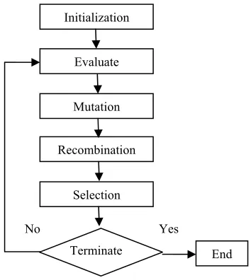
The detail procedure of DE was show in figure 1.

Fig. 1 The procedure of Differential evolution Yes

No

Initialization

Evaluate

Mutation

Recombination

Selection

(2)

The mutation is completed by the following formulation:

V, χ , F χ , χ , (1)

Where χ , , χ , and χ , are three different

individuals of the population, and combine with a mutation weighting factor (F) which is a parameter between [0,1] to obtain a Donor vectorV, .

The recombination is completed by the following formulation:

U,

V, , if rand CR

1

χ, , if

(2)

After the mutation operation, the donor vector will be use in recombination. Where CR is called crossover rate between [0,1], χ, denotes the old individual, and V,

denotes the new individual, if the random number is smaller than CR, we will chose V, ; on the contrary, we

will chose the original one, and obtain a trial vector finally. The selection is completed by the following formulation:

χ_, 3

Where χ, denotes the old individual and u,

denotes the trial vector which was obtained by recombination operation. Comparing these two vectors, the better one will be stayed and the other one will be eliminated. Finally, if the stopping condition is satisfied, DE will output the solution, if not, it will go back and repeat these three steps again.

B. Co-Evolutionary Mode

Co-Evolutionary mode was proposed by Ehrlich and Raven in 1964. The main concept of co-evolutionary is the relationship between butterfly and parasitic plant. Because the parasitic plant is inherence in nature, it is unable to resist the plague of vermin by their own; it produces the toxic substance to protect itself. Because of this toxic substance, butterfly also produces the resist mechanism and will become the effect of co-evolution [5].

Hilli proposed the other notion about the relationship between predators and predation [7]. Unlike the above mention, the main concept was competed with each other. Rosin and Belew also mentioned that co-evolution could not only represent one biological but also two or more. This method can improve the problems of traditional algorithm like premature convergence and high complex [6].

Based on the above described, the familiar model of co-evolution can be divided into two ways, one is cooperative evolution and the other is competitive co-evolution. This method was used in the genetic algorithm at the first time, and then Bergh and Engelbrecht was used this architecture on particle swarm optimization [8].

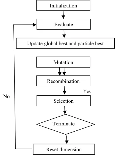
III. CO-EVOLUTIONARY DIFFERENTIAL EVOLUTION In this section, we will introduce about this co-evolution architecture for differential co-evolution. We proposed a novel DE, which was named CO-DE.

A. Co-evolutionary differential evolution

CO-DE also has three steps, including mutation, recombination and selection. In traditional DE, the mutation operation was used different individuals to obtain a donor vector, but this way can’t be used in co-evolution architecture as a result of the grouping may reduce the chance of select individuals. Thus, we aim to correct this disadvantage and use another mutation mechanism. After the evolution of CO-DE, we will proceed with the further improvement.

Fig. 2 The procedure of CO-DE

The basic process of CO-DE is exhibited in figure 2: (1)Initialization: Randomly initialize the population of individual for DE, where each individual contains d variables.

(2)Update the global best and particle best and compute the fitness value.

(3)Mutation: According the global best, particle best and a random individual to evolution a donor vector.

V, χ , F ρ

(4)Recombination: Perform recombination operation between each individual, and its corresponding mutant counterpart according to Eq. (2) in order to obtain each individual’s trial individual.

(5)Selection: Comparing the object vector and trial vector according to Eq. (3), the trial vector will be retain into next generation if it fitness were better than object vector.

u, if F u, F χ,

χ, otherwise

Yes No

Initialization

Evaluate

Mutation

Recombination

Selection

Terminate

Update global best and particle best

(3)

(6)Resetting: If the fitness has no change in five iterations, we will reset a dimension to each individual except the global best. We will randomly the each dimension of individuals of global and particle best, and take the Averaged. The related figure was show as in figure 3:

ρ

Fig. 3 The procedure of CO-DE

(7) If a stopping criterion is met, then output the solution; otherwise go back to Step (2).

IV. EXPERIMENT RESULT OF COMPARISONS To evaluate the performance of CO-DE, we will make two kinds of experiment. One of the experiment results, named co-evolution differential evolution without reset mechanism(CO-DEw), which was just added the co-evolution architecture in it. The second one, named CO-DE, which was added co-evolution and reset mechanism in the same time. Then, we will choose five benchmarks to authenticate this algorithm. The related parameter setting was showed as following:

A. Parameter setting

The related parameter setting was in table.

Table I CO-DE parameter setting

F 0.7 CR 0.2 Iter. 1000 upper_bound 100,5.12,600,32

low_bound -100,-5.12,-600,-32

NP(population size) 60

Dimension 10/20/30

Table II DE/rand1 parameter setting

F 0.5, 0.7

CR 0.9, 0.2

Iter. 1000 upper_bound 100,5.12,600,32

low_bound -100,-5.12,-600,-32

Dimension 10/20/30

Table III DE/rand1-to-best/1 parameter setting

F 0.5, 0.7

CR 0.3, 0.2

Iter. 1000 upper_bound 100,5.12,600,32

low_bound -100,-5.12,-600,-32

Dimension 10/20/30

B. Benchmark function

Table IV Benchmark function No Function

name

FUNCTION

f1 Sphere

_{( )}

2

i

f x

=

∑

x

f2 Rosenbrock

f3 Rastrigin

f4 Griewank

F5 Ackley

This section will compare the performance of CO-DE1, CO-DE2, DE/rand, and DE/rand-to-best/1. The experiment will show the different dimensions of these three methods. All of the experimental results were compared in Table V to VI.

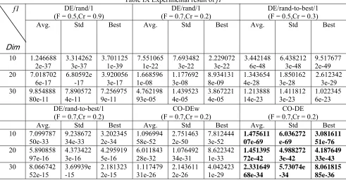
Tables VII to VIII exhibit the meaning and standard deviation of the function values by applying the six different algorithms to optimize the 10-D, 20-D, and 30-D numerical functions f1-f5, the convergence of CO-DE has an obvious great performance. In 30 dimensions of f2, although the particles are once stagnation, it still can escape out of the regional optimal solution. And at the same time, CO-DE also report that the great performance in low-dimension. In f3-f5, CO-DE also has great performance and the optimization can reach the best condition.

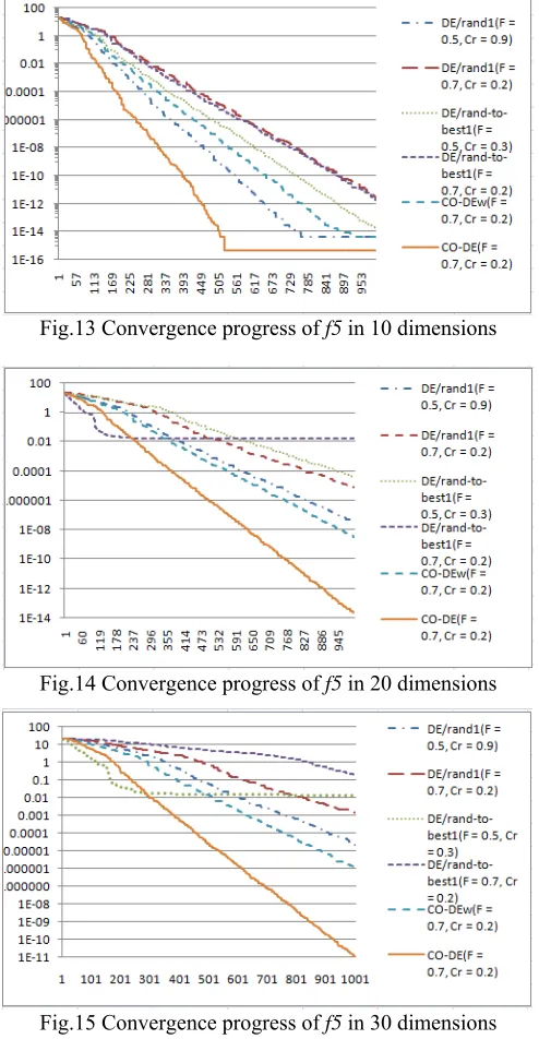
Figs.1 to 15 illustrate the convergence characteristics in terms of the best fitness value of the median run of each algorithm for functions – with D = 10 to 30. In the all figures, CO-DE also has fast convergence, especially the function of f3, f4, it even can reach the best solution 0 at 600~700 generations.

0.0038+(0.667 generation) = 0.619

0.899 0.0038...… .……….. …0.328

0.667 0.0123..… .……….. ….0.008

(4)

Table IX Experimental result of f1 f1

Dim

DE/rand/1

(F = 0.5,Cr = 0.9) (F = 0.7,Cr = 0.2) DE/rand/1 DE/rand-to-best/1 (F = 0.5,Cr = 0.3)

Avg. Std Best Avg. Std Best Avg. Std Best

10 1.246688

2e-37 3.3142623e-37 3.7011251e-39 7.5510651e-22 7.6934823e-22 2.2290723e-22 3.4421486e-48 6.4382123e-48 9.5176772e-49 20 7.018702

6e-17 6.80592e-17 3.9200563e-17 1.6685961e-08 3e-08 1.177692 8.9341318e-09 1.3436544e-28 1.8501623e-28 2.6123423e-29 30 9.854888

80e-11 7.8905724e-11 7.2569759e-11 4.76219893e-05 4e-05 1.439523 3.8672214e-05 1.21388814e-23 1.4118123e-23 1.0223456e-23 DE/rand-to-best/1

(F = 0.7,Cr = 0.2) (F = 0.7,Cr = 0.2) CO-DEw (F = 0.7,Cr = 0.2) CO-DE

Avg. Std Best Avg. Std Best Avg. Std Best 10 7.099787 50e-33 9.238672 34e-33 3.202345 2e-34 1.096994 58e-52 2.751463 2e-50 7.812444

3e-52 1.47561107e-69

6.036272 e-69

3.081611 51e-76 20 5.890858

97e-16 4.3734223e-16 4.2959195e-16 6.01184328e-32 1.07649234e-31 8.6223421e-33 1.45139572e-42

4.988272 3e-42

4.187649 33e-43 30 8.066742

52e-15 3.69939e-15 2.1813232e-15 1.11747931e-26 2.1436112e-26 4.0424231e-29 2.33164968e-34

5.73074e -34

8.061815 85e-36

Table X Experimental result of f2

f2

Dim

DE/rand/1 (F = 0.5,Cr = 0.9)

DE/rand/1 (F = 0.7,Cr = 0.2)

DE/rand-to-best1 (F = 0.5,Cr = 0.3)

Avg Std Best Avg. Std Best Avg. Std Best

10 9.042799

6e+00 1.3810258e+00 2.8481244e+00 4.277833e+00 1.133932e+00 3.733589e+00 3.506e+00 1.86e+00 2.816654e+00 20 1.583842 5e+01 1.303223 4e+00 1.410791 8e+01 1.708272 e+01 1.294251 e+00 1.677287 e+01 1.5163e+ 01 1.573e+0 0 1.5111e+ 01 30 3.97234e

+01 2.7472590e+00 2.6297142e+01 5.943572e+01 e+01 1.417247 3.569013e+01 2.511773e+01 9.098447e-01 2.19344e+01 DE/rand-to-best/1

Avg. Std Best Avg. Std Best Avg. Std Best 10 6.914395

6e+00 1.2496468e+00 5.2976756e+00 2.1834635e+00 3.47630342e-01 1.5977927e+00 1.3816354e+00

3.476303 42e-01

1.260033 e+00 20 1.872651

0e+01 7.35167941e-01 1.5378953e+01 1.3027426e+01 4.066192e+00 9.3715216e+00 4.9093048e+00

4.066192 e+00 2.122857 6e+00 30 2.610758 0e+01 6.679879 73e-01 2.48564e +01 2.301400 0e+01 1.015797 4e+00 1.702273

8e+01 1.5862197e+01

5.138547 2e+00

(5)

Table XI Experimental result of f3

f3

Dim

DE/rand/1

(F = 0.5,Cr = 0.9) (F = 0.7,Cr = 0.2) DE/rand/1 (F = 0.5,Cr = 0.3) DE/rand-to-best1

10 1.515455

7e+01 5.0083099e+00 5.9697543e+00 4.582005e+00 2.069054e+00 3.157312e+00 1.658265e-01 3.77138e-01 0 20 8.735991

8e+01 1.1258444e+01 7.210975e+01 7.138424e+01 e+00 7.833339 5.01659e+01 3.651900e+00 2.134871e+00 2.474107e+00 30 1.672739

8e+02

2.342926 e+01

1.538393 e+02

1.439317 e+02

1.142349 e+01

1.112356 e+02

5.31850e +01

9.047401 e+00

4.683711 e+01 DE/rand-to-best1

5e+00 6.03913056e-01 4.841918e-02 2.467478e-12 1.279852e-11 5.467626e-12 0 0 0 20 1.917336

0e+01 2.6694871e+00 1.5158623e+01 3.14697e-01 5.514240e-01 3.519269e-04 0 0 0 30 6.601837

1e+01

4.249302 6e+00

6.202762 9e+01

7.130986 e+00

2.756044 e+00

1.568877

e+00 9.62540e-012

1.75735e -12

0

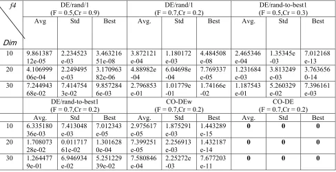
Table XII Experimental result of f4

f4

Dim

DE/rand/1

10 9.861387

12e-05 2.234523e-03 3.46321651e-08 3.872121e-04 e-03 1.180172 4.484508e-08 2.465346e-04 1.35345e-03 7.012168e-13 20 4.106999

06e-04 2.249495e-03 3.17096382e-06 4.88982e-04 -04 6.04698e 7.769337e-05 1.231684e-03 3.813249e-03 3.7636560-14 30 7.244943

68e-02 7.4147543e-02 9.8572846e-03 2.796853e-01 -01 1.01779e 1.74166e-02 1.187543e-01 5.260329e-02 7.396161e-03 DE/rand-to-best1

36e-03

7.413048 e-03

7.012343 e-05

2.975617 e-05

1.875291 e-03

1.443289

e-15 0 0 0

20 1.708073

28e-02 0.01171761e-02 1.3016280e-04 7.399251e-05 2.256913e-03 1.432187e-14 0 0 0 30 1.264477

(6)

Table XIII Experimental result of f5 f5

Dim

DE/rand/1

10 3.961202

23e-14 2.40704e-30 3.99680288e-15 4.111851e-12 e-13 5.211912 3.068177e-12 3.118624e-14 1.203523e-30 1.376676e-14 20 2.971261

60e-07

1.594448 65e-07

3.375352 75e-08

6.512781 e-06

1.636534 e-06

4.306734 e-06

5.487412 e-02

3.005579 e-01

3.772342 e-05 30 4.986823

25e-05 2.0370623e-05 2.00096919e-05 1.563648e-03 -03 2.28501e 1.420190e-03 1.055528e+00 1.98817e-15 1.316815e-02 DE/rand-to-best1

13e-11 1.38607e-10 1.86561877e-12 4.196802e-15 2.407042e-30 3.994832e-15 2.575717e-15

1.77022e -15

4.440892 e-16 20 3.752083

e-01

5.874323 4e-01

1.724047 2e-02

5.983143 e-09

2.270742 e-09

3.177220

e-09 9.878379e-13

6.48634e -13

2.176037 e-14 30 1.563805

0e+00 5.47997092e-01 1.78377498e-01 1.249945e-06 2.73222e-07 1.038910e-06 6.128431e-10

3.03759e -10

3.612494 e-11

Fig.1 Convergence progress of f1 in 10 dimensions

(7)

(8)

C. Comparison with other researches

We will compare with three different researches, one was named KCPSO[9], which was combined the co-evolution architecture on particle swarm optimization. The second one was named PSODE[10], which was combined both differential evolution and particle swarm optimization, and it was also a kind of co-evolution architecture. The third one was named SaDE[11], which was improved by self- adaptive. And the result was compared in Table XIV.

The result showed that five different improve methods, and they both have 10-D and 30-D to optimize numerical functions f1-f5, and all results showed that our CO-DE has great performance except the function f2. In f2, SaDE has the best solution that the meaning of function value was about 0.3. And it was greater than other algorithms, but in other numerical function, CO-DE still has distinct improvement.

Table XV compare with other algorithms

V. COCLUSIONS

In this paper, cooperative CO-DE is proposed to solve global optimization problems. The contribution of this paper is mainly in the following two aspects: (1) through the co-evolutionary, the particles can explored the search space more in depth and reduce the speed for convergence. (2) A reset mechanism was proposed to enhance the performance and avoid the stagnation. This mechanism can prevent the above problems effectively and avoid increasing the complex of algorithm.

Due to CO-DE was an improved architecture, it may combine with other improved methods, such as improvement of parameters (F or CR) or other evolutionary mechanisms.

REFERANCES

[1] Storn, R., Price, K., “Minimizing the real functions of the ICEC'96 contest by differential evolution “, Evolutionary Computation, 1996., Proceedings of IEEE International Conference on 20-22 May 1996 Page(s):842 – 844

[2] Storn, R. and Price, K., “Differential Evolution- a simple and efficient adaptive scheme for global optimization over continuous spaces,” Technical Report TR-95-012, ICSI. [3] Price K., “Differential Evolution: A Fast and Simple

Numerical Optimizer,” 1996 Biennial Conference of the

North American Fuzzy Information Processing Society,

Jun. 1996, pp.524-527.

[4] Amin N., Hong W., “Co-evolutionary Self-Adaptive Differential Evolution with a Uniform-distribution Update Rule”, Intemational Symposium on Intelligent Control Munich, Germany, October 4-6,2006.

[5] Ehrlich, P.R., P.H. Raven, 1964, “ButterDies and plants: a study in coevolution,” Evolution vol.18 pp586–608.

[6] Rosin, C.D. and Belew, R.K., “New methods for Competitive Coevolution.” Evolutionary Computation 1997, 5:1-30.

[7] Hillis, W.D., “Coevolving parasites improve simulated evolution as an optimization procedure,” In Langton, C.G., Taylor, C., Farmer, J.D., & Rasmussen, S. (Eds), Artificial Life II , Redwood City, CA: Addison Wesley. 1992, pp.313-324.

[8] F. van den Bergh, A.P. Engelbrecht,“ A cooperative approach to particle swarm optimization, ” IEEE Transaction on Evolutionary Computation 8 (3), 2004, 225–239.

(9)

[10] N. Ben and L. Li., “A Novel PSO-DE-Based Hybrid Algorithm for Global Optimization”, Computer Science, Vol. 5227, 2008, pp. 156-163.

[11] A.K. Qin, V.L.Huang, and P.N. Suganthan, “Differential Evolution Algorithm With Strategy Adaptation for Global Numerical Optimization”,IEEE transactions on evolutionary computation, vol.13,No 2, April 2009.

Wei-Ping Lee received the Ph.D. degrees in Institute of Computer Science and Information Engineering from National Chiao Tung University, Hsinchu, Taiwan, R.O.C.

Currently, he has been an Assistant Professor in the Department of at Chung Yuan Christian University Chung li, Taiwan, R.O.C. His research interests include the global optimization of evolutionary algorithms, data mining and AI applications.

Wan-Jou Chien Chang-Yu Chiang received the master degree in Information Management from Chung Yuan Christian University, Chung li, Taiwan, R.O.C.