www.the-cryosphere.net/10/1297/2016/ doi:10.5194/tc-10-1297-2016
© Author(s) 2016. CC Attribution 3.0 License.
Development and calibration of an automatic spectral albedometer
to estimate near-surface snow SSA time series
Ghislain Picard1,2, Quentin Libois1,a, Laurent Arnaud1, Gauthier Verin1, and Marie Dumont3
1UGA/CNRS, Laboratoire de Glaciologie et Géophysique de l’Environnement (LGGE) UMR 5183, Grenoble, 38041, France 2ACE CRC, University of Tasmania, Private Bag 80, Hobart, TAS 7001, Australia
3Météo-France – CNRS, CNRM – GAME UMR 3589, Centre d’Études de la Neige, Grenoble, France
anow at: ESCER Centre, Department of Earth and Atmospheric Sciences, Université du Québec à Montréal (UQAM), Montréal, Canada
Correspondence to:Ghislain Picard ([email protected])
Received: 17 November 2015 – Published in The Cryosphere Discuss.: 18 January 2016 Revised: 4 May 2016 – Accepted: 27 May 2016 – Published: 21 June 2016
Abstract. Spectral albedo of the snow surface in the visible/near-infrared range has been measured for 3 years by an automatic spectral radiometer installed at Dome C (75◦S, 123◦E) in Antarctica in order to retrieve the specific surface area (SSA) of superficial snow. This study focuses on the un-certainties of the SSA retrieval due to instrumental and data processing limitations. We find that when the solar zenith an-gle is high, the main source of uncertainties is the imperfect angular response of the light collectors. This imperfection in-troduces a small spurious wavelength-dependent trend in the albedo spectra which greatly affects the SSA retrieval. By modeling this effect, we show that for typical snow and illu-mination conditions encountered at Dome C, retrieving SSA with an accuracy better than 15 % (our target) requires the difference of response between 400 and 1100 nm to not ex-ceed 2 %. Such a small difference can be achieved only by (i) a careful design of the collectors, (ii) an ad hoc correction of the spectra using the actual measured angular response of the collectors, and (iii) for solar zenith angles less than 75◦. The 3-year time series of retrieved SSA features a 3-fold de-crease every summer which is significantly larger than the estimated uncertainties. This highlights the high dynamics of near-surface SSA at Dome C.
1 Introduction
The summer surface energy budget on the ice sheets is largely controlled by the absorption of solar energy by snow
(Van As et al., 2005; Ettema et al., 2010). The latter is de-termined by the downward irradiance reaching the surface and by snow albedo. With solar irradiance of several hun-dreds of W m−2during daylight, a persistent change of 1 % of the albedo represents an energy comparable with the glob-ally averaged radiative forcing caused by CO2concentration increase since preindustrial time (1.82 W m−2, Myhre et al., 2009). While planetary albedo change is not expected to ex-ceed a 0.1 % (Myhre et al., 2009), local changes can be much larger due to the dependence of snow albedo on multiple factors including snow grain size and shape, surface rough-ness, snow depth, and the amount of light-absorbing impuri-ties such as black carbon, dust, and biological pigments (e.g., Warren and Wiscombe, 1980; Warren et al., 1998; Aoki et al., 2000; Dumont et al., 2010; Zhuravleva and Kokhanovsky, 2011; Stibal et al., 2012; Goelles et al., 2015). These factors vary in space and time depending on the atmospheric condi-tions and are controlled by numerous processes giving rise to complex snow–albedo feedback loops between the snow cover and the atmosphere (Curry et al., 1995; Qu and Hall, 2007; Picard et al., 2012). In Antarctica, snow grain size is the main factor controlling the albedo along with the illumi-nation conditions (solar zenith angle (SZA) and cloud cover) and surface roughness while the impurity content is usually low (Warren et al., 2006). Investigating the feedback loops thus requires long-term and accurate observations of albedo and snow properties.
Sur-face Radiation Network (BSRN) stations and some auto-matic weather stations deployed by the Institute of Marine and Atmospheric research (Utrecht University) provide time series of broadband albedo measured using upward- and downward-looking pyranometers. In addition, these sensors are subject to many artifacts such as imperfect response at high solar zenith angle, leveling and frost, which are difficult to correct (van den Broeke et al., 2004; Bogren et al., 2016). Retrieving broadband albedo from remote sensing is not a straightforward alternative. It requires atmospheric correc-tion, spectral extrapolation from a limited number of spectral bands, and angular extrapolation of the bi-conical measure-ments to get hemispherical surface reflectance (Stroeve et al., 2006). The latter is challenging because the bi-directional reflectance of snow is much more sensitive to grain shape (Dumont et al., 2010) and surface roughness (Kuchiki et al., 2011) than hemispherical reflectance (i.e., albedo), thus in-troducing extra unknown variables that need to be estimated somehow. Moreover, satellite data cannot be used under cloudy conditions or when the sun zenith angle is too high (Wang and Zender, 2010; Schaaf et al., 2011). Despite many satellite overpasses per day in polar regions, the time series are discontinuous and snowfalls, which are periods of great albedo change, are systematically missed.
Measuring snow grain size is difficult as well. Estimat-ing the maximal extent of the dominant crystals usEstimat-ing hand-lens or binocular is the most widely used technique to mea-sure grain size (Fierz et al., 2009; Aoki et al., 2000; Pirazz-ini et al., 2015). However, not only is it known to be im-precise and operator dependent, but also it cannot be auto-mated for unmanned monitoring of grain size evolution. Re-cent advances in field measurement of the specific surface area (SSA; the surface area of the air–ice interface per unit of mass of snow) – which is equivalent to the optical ra-dius commonly used in remote sensing (Grenfell and War-ren, 1999; Nolin and Dozier, 2000; Jin et al., 2008) – offer an attractive alternative. Examples of instruments and meth-ods include contact spectroscopy (Painter et al., 2007), near-infrared photography (Matzl and Schneebeli, 2006), DU-FISSS and IceCUBE (Gallet et al., 2009) and POSSSUM and ASSSAP (Arnaud et al., 2011). These techniques be-ing based on optical measurements of the snow reflectance in the near or short wave infrared, it is arguable whether they provide data more related to albedo or a proper geometrical metric of the snow micro-structure. Several theoretical stud-ies have indeed shown the significant influence of the snow crystal shape on the albedo (Macke and Mishchenko, 1996; Neshyba et al., 2003; Kokhanovsky and Zege, 2004; Picard et al., 2009) and on the e-folding depth (Libois et al., 2013) but no clear experimental evidence of this effect has been given yet for snow on the ground (Gallet et al., 2009; Li-bois et al., 2014b). In fact, these optical techniques have been shown to be accurate within 15 % when compared with inde-pendent measurements using methane adsorption or micro-computed tomography techniques (Matzl and Schneebeli,
2006; Domine et al., 2006; Gallet et al., 2009). This accu-racy is sufficient to achieve a 1 % accuaccu-racy of broadband albedo (Gardner and Sharp, 2010) which is considered to be adequate for climate study (Bogren et al., 2016). Inten-sive campaigns of SSA measurements have provided new in-sight of the snow metamorphism in the Alps and in Antarc-tica over seasons and have allowed refined evaluation of de-tailed snow model predictions (Picard et al., 2012; Morin et al., 2013; Roy et al., 2013; Libois et al., 2015). However, these techniques still require an operator which is often a limitation, particularly in Antarctica. Optical satellite remote sensing has been used to retrieve optical radius (e.g., No-lin and Dozier, 2000; Painter et al., 2009; Negi et al., 2011; Mary et al., 2013) in particular in Antarctica (Scambos et al., 2007; Jin et al., 2008). Mary et al. (2013) and Tanikawa et al. (2015) give an overview of the numerous existing algorithms. Obtaining grain size on a large spatial extent and for many years is of great interest, but attaining an accuracy similar to that of field techniques requires to overcome several addi-tional defects that are specific to space-borne sensors and are in fact very similar to those faced for albedo retrieval. Mi-crowave remote sensing is not subject to these issues but, as far as albedo study is concerned, only the highest available frequencies could be able to provide superficial grain size (Picard et al., 2012). However, the technique proposed by Pi-card et al. (2012) is specific in many ways to the conditions of the Antarctic Plateau and requires additional assumptions about the density and temperature of superficial snow com-pared to the optic domain (Wuttke et al., 2006).
Ground-based observation of spectral albedo has several advantages compared to broadband measurement: it can pro-vide a finer understanding of the albedo variations and can be used to estimate SSA using similar principles to those used in remote sensing and by the optical techniques mentioned above. It is also easier to assess the data quality or develop corrections by exploiting the spectral signature. Many spec-tral albedo measurements have been conducted in Antarctica (e.g., Grenfell et al., 1994; Hudson et al., 2006; Hudson and Warren, 2007; Marks et al., 2015; Pirazzini et al., 2015) but they were limited to short-term campaigns and the tempo-ral evolution was not the priority. Long-term monitoring of spectral albedo requires fully automatic instruments with a good robustness to cope with the Antarctic conditions (Wut-tke et al., 2006; Salzano et al., 2016). With the advent of cheaper and compact spectrometers free of mechanical parts (Kantzas et al., 2009; Nicolaus et al., 2010), operating such instruments in Antarctic conditions is becoming easier.
target uncertainty of 15 %, as claimed to be reached by man-ual devices – near-infrared photography (Matzl and Schnee-beli, 2006), DUFISSS (Gallet et al., 2009), and POSSSUM (Arnaud et al., 2011) – and considering it is difficult to per-form better than those man-operated tools. Theoretical mod-eling of the imperfections of the instrument is used to help in this analysis and also to provide quantitative recommen-dations for the design of future spectral radiometers. Simu-lations are also used to explore the representativeness of the retrieved SSA. The geophysical interpretation of the 3-year SSA time series obtained with our instrument and its com-parison to snow model simulations are addressed in Libois et al. (2015).
Section 2 describes the retrieval of SSA from spectral albedo and uncertainties induced by instrumental artifacts. Section 3 presents the instrument deployed at Dome C and the data processing to obtain calibrated albedo. The 3-year time series of retrieved SSA is presented and analyzed in Section 4. Discussion and conclusion are provided in the last section.
2 Theory
In this section, we present the algorithm to retrieve SSA from observed spectral albedo and evaluate the uncertainties re-sulting from working hypothesis and instrumental artifacts.
2.1 Retrieval of specific surface area from spectral albedo
Snow SSA at the surface is obtained by fitting a theoreti-cal albedo model with SSA as the main unknown to ob-served albedo spectra over some range of wavelengths. To keep the number of unknowns moderate in order to pre-vent unstable optimization, the following assumptions are made. (1) The snowpack is horizontally and vertically ho-mogeneous, which means only one SSA value is retrieved. (2) The surface is flat. Roughness which tends to weaken the solar zenith angular response of the snow is neglected (Warren et al., 1998). (3) The surface and the sensor are per-fectly horizontal. (4) Snow phase function and single scatter-ing albedo are implicitly described by the asymmetry factor, absorption enhancement parameter, and SSA (Kokhanovsky and Zege, 2004). The values of asymmetry factor and absorp-tion enhancement parameter are assumed constant. (5) Snow is clean or contains sufficiently small quantities of impurity not to impact the albedo in the considered wavelength range. This is usually the case in Antarctica (Grenfell et al., 1994).
In these conditions, the analytical asymptotic radiative transfer (ART; Kokhanovsky and Zege, 2004; Negi et al., 2011) is valid and gives the directional and diffuse
hemi-spheric reflectancesαdiffandαdiras a function of SSA:
αdiff(λ)=exp −4
s
2Bγ (λ)
3ρiceSSA(1−g)
!
(1)
αdir(λ, θ )
=exp −12
7 (1+2 cosθ )
s
2Bγ (λ)
3ρiceSSA(1−g)
!
, (2)
whereθ is the solar zenith angle, ρice=917 kg m−3 is the ice density at 0◦C, andγ (λ)is the absorption coefficient of ice, taken from Warren and Brandt (2008).B=1.6 andg=
0.85 are, respectively, the absorption enhancement parameter and the asymmetry factor values suggested by Libois et al. (2014b).
Considering that observed albedo is composed of a direct and diffuse component, the model reads
α1-param(λ, θ )=hrdiff(λ, θ )αdiff(λ)
+1−rdiff(λ, θ )αdir(λ)i, (3)
whererdiff(λ, θ )is the ratio of diffuse over direct irradiance and is supposed to be known. This simple model is called hereinafter “one-parameter model” because SSA is the only unknown. However, it is not the most suitable because albedo measurements are subject to various artifacts, such as varia-tions of the illumination or poor cross-calibration between the downwelling and upwelling measurements, slopes of the surface, etc., sometimes even resulting in values larger than 1 (Pirazzini et al., 2015). To cope with artifacts that do not de-pend on wavelength, a free wavelength-indede-pendent scaling parameterAis introduced:
α2-param(λ, θ )=Ahrdiff(λ, θ )αdiff(λ)
+1−rdiff(λ, θ )αdir(λ)i. (4) This two-parameter model is more flexible but to avoid over-fitting, we discard spectra that would result inAout of the range 0.9–1.1.
The fit is performed with a nonlinear least squares method (provided by the Python scipy.optimize.leastsq function) to minimize the squared difference between the model and ob-served spectrum.
2.2 Vertical representativeness of retrieved SSA values Assuming the snowpack is vertically homogeneous and re-trieving a single bulk SSA stabilizes the fit. However, this implies to interpret the retrieved value with caution. There is indeed some evidence of significant vertical gradient in the topmost centimeter in Antarctica. Grenfell et al. (1994) found it necessary at the South Pole to add a thin layer of very small snow grains (SSA larger than 100 m2kg−1) on the surface in their radiative transfer calculations in order to match their albedo measurements. They attributed this to the deposition of snow particles having been shrunk by sublimation during blowing snow events. Carmagnola et al. (2013) at Summit in Greenland use spectral data in the visible, near- and short-wave infrared and found that tuning the surface layer SSA helped to improve the agreement with the observations but did not explore values as high as Grenfell et al. (1994) did. In contrast, Gallet et al. (2011) measured SSA vertical pro-files at Dome C and obtained radiative transfer calculations in agreement with Hudson et al. (2006) observations with-out adding such a layer. Using snowpack numerical mod-eling, Libois et al. (2015) obtained SSA profiles at Dome C with such a significant gradient near the surface. This is particularly remarkable as their simulations do not consider some processes susceptible to bring small grains on the sur-face such as shrinking of airborne particles by sublimation or clear-sky precipitation (a.k.a. diamond dust).
Because of this gradient, it is important to know over which thickness the retrieved SSA is representative. Unfor-tunately, there is no simple answer because the penetration depth of radiation in snow depends not only on the wave-length but also on the vertical profile of snow properties, including SSA itself and density, which are both unknown. Furthermore, the estimated SSA value is not a simple aver-age over a given thickness but is a weighted averaver-age with a kernel function decreasing with depth. This function has an exponential form for homogeneous snowpack but is more complex otherwise.
Only multi-layer radiative transfer calculations can give a precise estimation of the sensitivity–depth relationship when SSA and density profiles are known. To evaluate this rela-tionship in the simple case of an homogeneous snowpack, we proceed as follows: the two-stream radiative transfer model TARTES (Libois et al., 2013) is run considering a semi-infinite medium with fixed SSA and a density of 270 kg m−3 (typical mean surface conditions at Dome C; Libois et al., 2014a). A layer with variable thickness h is added on top of it, with the same properties, excepted that a small per-turbationδSSA is added to the SSA. The relative contribu-tion of the uppermost layer to the albedo is then defined as the quantity(α(h)−α(0))/(α(∞)−α(0)), whereα(h)is the albedo calculated by TARTES for the thickness h and av-eraged over the wavelength range used by Autosolexs (au-tomatic solar extinction in snow) (700–1050 nm). The ac-tual value of δSSA does not change the final result due to
Figure 1.Contribution of the uppermost layer of a semi-infinite snowpack to the albedo averaged over the range 700–1050 nm (plain line) and at 1310 nm (dash line) as a function of the layer thickness.
the normalization, as long as it is small (e.g., +1 m2kg−1). The contribution is shown in Fig. 1 (plain line) as a func-tion of h for different SSA values. Results show that the uppermost 10 mm snow layer contributes to nearly 60 % of the albedo for SSA of 20 m2kg−1and 85 % for higher SSA of 100 m2kg−1. Conversely, the layer contributing to 80 % of the signal is 18, 12, and 8 mm thick for SSA of 20, 50, and 100, respectively. We can conclude that 1 cm is a rea-sonable approximation for Dome C conditions, which gives a more quantitative meaning to the term “near-surface” used throughout this article.
For comparison, we also run similar simulations at 1310 nm, a wavelength commonly used by device to mea-sure SSA (Gallet et al., 2009; Arnaud et al., 2011) (dashed line in Fig. 1). In this case, most of the signal comes from the uppermost 5 mm in any common conditions. Note that the penetration depth is inversely proportional to density so that the thickness values presented here should be multiplied by about 2 in case of fresh snow or surface hoar.
observations in Sect. 3. In both cases, to quantify the impact on the estimation of the SSA, we perform simple and ideal-ized numerical experiments as follows: we first compute the perfect albedo spectrum with the model described in Eq. (1) for a given SSA (called true SSA) and perturb it to mimic the considered artifact. Then, we retrieve the SSA using the algorithm described in Sect. 2.1 and deduce the error as the difference between the estimated and true SSA.
2.3.1 Offset
We consider the true reflected and incident radiance spectra
Sref(λ) andSinc(λ) are affected by a constant bias d. The measured albedo is calculated by
α(λ)= S
ref(λ)+d
Sinc(λ)+d. (5)
Dividing by the incident radiance makes explicit the true albedo,αtrue:
α(λ)=
αtrue+ d
Sinc(λ)
1+ d
Sinc(λ)
. (6)
For the incident spectrum Sinc(λ), we choose a Gaussian shape that mimics the observations (Sect. 3.3):
Sinc(λ)=Smodeexp
"
−
λ−680nm 270nm
2#
. (7)
The amplitude of the spectrumSmodeis usually of the order of the resolution of the digital-to-analog converter of the ra-diometer (216 in our case) if the integration time is optimal. We defined0=d/Smode, the relative contribution of the off-set with respect to the spectrum amplitude. We then estimate the SSA from the perturbedα(λ)spectrum and calculate the difference with respect to the true SSA.
Figure 2 shows the SSA error as a function of the relative offsetd0ranging from 0 (perfect instrument) to 2 % for sev-eral SSA values. The result is nearly independent of the true SSA. To meet the 15 % accuracy criteria, the offset needs to remain underd0=1 %. For a spectrometer, this offset can gen-erally be estimated using dark pixels (pixels receiving any light so that S(λ)=0). Since their signal-to-noise ratio is usually much better than 1:100, the offset correction should not in most case be an obstacle to achieve the targeted accu-racy.
2.3.2 Chromatic aberration
To investigate the impact of chromatic aberration, we con-sider the true albedo αtrueis multiplied by a linear function of the wavelength:
α(λ, θ )=
1−bλ−λ0 λ1−λ0
αtrue(λ, θ ), (8)
Figure 2.Theoretical calculation of the relative error in SSA due to an offset in the incident and reflectance spectra for SZA=60◦. The dashed line shows the 15 % target accuracy discussed in the paper.
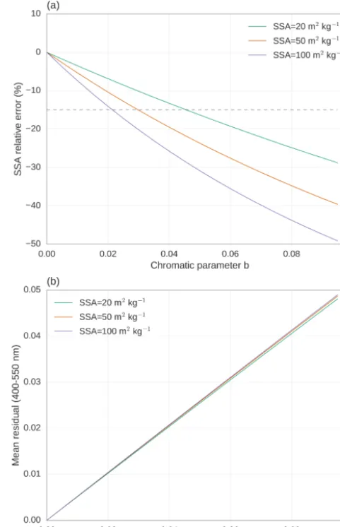
whereb controls the slope of the wavelength dependence. The limits λ0=400 nm and λ1=1100 nm are chosen so that the instrument is assumed perfect at 400 nm in the blue andbrepresents the relative response difference between the upward- and downward-looking channels at 1100 nm. Fig-ure 3 illustrates the results with true SSA of 50 m2kg−1and
b=0.05 (actual values ofbare given in this section and in Sect. 3). Note that the SSA estimation only uses data between 700 and 1050 nm. The retrieved SSA is 38.2 m2kg−1 with the two-parameter model and 27.6 m2kg−1 with the one-parameter model. This corresponds to relative errors of 24 and 45 %, respectively. The two-parameter model is clearly better, which can be explained by the fact that it is insensi-tive to the scaling of the albedo and depends mostly on the spectral variations of albedo within the range used for the op-timization. However, this error is larger than the 15 % target accuracy in SSA.
er-Figure 3.Simulations of albedo spectrum for SZA=60◦. A per-fect albedo spectrum for an homogeneous snowpack with SSA of 50 m2kg−1(black) is perturbed by a factor linearly decreasing from 1 at 400 nm to 1−bat 1100 nm withb=5 % (green) and used as an observation to estimate SSA with the one-parameter (violet thin dash) and two-parameter models (orange, long dash). Estimated val-ues are shown in the legend along with the relative error.
ror and the mean difference over the range 400–550 nm as a function of the chromaticity parameterb for several SSAs. The error varies almost linearly with b and the slope in-creases with SSA. Hence, to attain the target accuracy of 15 %, the chromatic parameter should not exceed about 0.04 for SSA=20 m2kg−1and 0.02 for SSA=100 m2kg−1. Fig-ure 4b shows the nearly univocal relationship betweenband the mean residual. This suggests that mean residual values under 0.01 indicate a chromaticitybbetter than 0.02 and thus an SSA accuracy better than 15 %, thereby providing a fast and simple spectra quality check criteria.
We implemented this criteria in our algorithm as fol-lows: (1) predict the albedo spectrum with the two-parameter model using the optimal SSA andAparameters obtained by fitting the model to the observed spectrum in the range 700– 1050 nm, (2) calculate the mean difference in the range 400– 550 nm, and (3) reject the spectrum if this difference is larger than 0.01. This filter works at Dome C where snow is clean but would not work in the presence of light absorbing im-purities because the latter cause a decrease of the albedo in the blue/green domain (Warren, 1982), which would result in systematic rejection by the filter.
Several artifacts result in chromatic aberration. Leveling of the collector is one of them. Tilt angle δof the collector with respect to the horizontal indeed tends to affect albedo by a scalingη(λ, θ )that can be written according Bogren et al. (2016) and Grenfell et al. (1994):
η(λ, θ )≈1−rdiff(λ, θ )
cos(θ−δ)
cos(θ ) −1
, (9)
Figure 4. (a)Theoretical calculation of the relative error in SSA due to the chromatic aberration of the spectrometer as a function of the parameterbdefined in Eq. (8) for SZA=60◦. The dashed line shows the 15 % target accuracy discussed in the paper.(b) Relation-ship betweenband the residual between the observed and estimated albedo averaged over the range 400–550 nm.
where the diffuse term error has been neglected as suggested by Bogren et al. (2016) findings. Tilt in the direction of the sun (worse case) is considered. Assuming the errors are small enough to be treated as perturbations,b can be deduced as follows:
b≈η(λ1, θ )−η(λ0, θ ), (10)
≈rdiff(λ1, θ )−rdiff(λ0, θ )
cos(θ−δ)
cos(θ ) −1
. (11)
These results highlight the crucial role of the leveling of the instrument. Other artifacts resulting in chromatic aberration are addressed in Sect. 3.4 on practical examples.
3 Measurements of spectral albedo
A specific instrument has been developed to measure the spectral albedo of the surface at Dome C. The following sub-section describes the instrument, details on the light collec-tors (or fore optics) and data processing steps.
3.1 Autosolexs instrument
We designed and assembled an instrument composed of sev-eral commercial and homemade components. The main spec-ifications driving the design were the robustness to work in Dome C harsh environment for several years and the ability to acquire not only albedo (incident and reflected radiation) but also the radiation within the snow at several levels (not used in this study), thus requiring a spectrometer with many inputs. The instrument is named Autosolexs because of the latter application.
Figure 5 shows pictures of the visible aboveground part of the system which comprises two heads for albedo measure-ments at about 2 m above the surface. Due to snow accumu-lation, this height has decreased at an averaged rate of about 10 cm per year since the installation. Each head is equipped with two light collectors looking upward and downward. The collected radiation is transmitted by 6 m long fiber optics (core diameter of 400 µm) to the rest of the device that is buried under the snow. Neither electronic nor fragile parts are aboveground.
The instrument scheme is depicted in Fig. 6. The fibers coming from the heads are directly connected to the inputs of a 16-to-1 optical switch (FiberSwitch® mol 1×16 19 in 2 hu by Leoni). Using a mechanic–optical module driven by a digital interface, it links in a few milliseconds one of the 16 inputs to the output with a reproducibility better than 0.03 dB according to the manufacturer. This corresponds to about 0.7 % uncertainty for the irradiance which in the worse case translates to 1.4 % for the albedo. The output of the switch is connected to a 1-to-2 splitter that transmits radiation to two spectrometers (MAYA2000 PRO, Ocean Optics). One covers the visible and near-infrared and the second one is dedicated to the near-infrared. Only the former is used in this study. It gives signal above the noise level in the range 350–1050 nm with an effective spectral resolution of 3 nm. One of the in-puts of the optical switch is obstructed so it measures dark conditions that are used to correct the offset present in the spectrometer acquisitions. The instrument container is ther-malized at+10±2◦C, which is necessary for nominal oper-ation and stability of the spectrometers.
An embedded computer controls the optical switch and the spectrometers and schedules the acquisition. Every 12 min, a
12 October 2014
11 November 2014
Figure 5.Pictures of the snow surface under Autosolexs head (head 1 is on the left) on 12 October and 11 November 2014.
complete sequence of measurements is performed in the fol-lowing order: head 1 (incident and then reflected channels), head 2 (incident and then reflected channels), buried fibers, heads 1 and 2 again, and at last dark. Each measurement takes 10–20 s. An automatic camera is connected to the computer to take one picture per sequence like those shown in Fig. 5. This provides qualitative but very useful information on the state of the snow surface and the presence of frost on the light collectors. The system is connected to the power supply of the Concordia station – the power consumption is typically around 50 W – and to the network to send data in near-real time.
down-Spectrometer
300 - 1100nm Spectrometer700 -1100nm 16 – channel optical
multiplexer Albedo head 1
upward downward downward
upward Albedo head 2
Embedded PC
d
a
ta data
Internal black
Y-separator
Thermalized enclosure +10°C
Buried fibers
Figure 6.Principle of Autosolexs. The dotted rectangle represents the thermalized container that is buried in the snow. The plain curved lines represent fiber optics, the fibers buried in snow (gray) are not used in the present study.
welling spectral irradiances, and the flux is the energy (per unit of surface, of time, and of wavelength) crossing an hor-izontal surface. To measure flux, the collector must have a so-called cosine response so that the energy coming with an oblique direction is weighted by the cosine of the zenith an-gle (Grenfell et al., 1994; Morrow et al., 2000).
In principle, a flat surface which transmits a constant pro-portion of the incident beam whatever its direction acts as a perfect collector. For this reason, collectors are often made of a flat disk of highly diffusing material like sintered teflon grains. Nevertheless, teflon grains, like snow grains, have a strong forward scattering behavior so that flat collectors are more reflective at grazing angles than for the normal inci-dence. As a result, they transmit less at grazing angles than required for a perfect cosine response. In clear-sky condi-tions, when the sun is low on the horizon, the upward-looking collector tends thereby to underestimate the incoming flux. In contrast, the irradiance reflected by the snow is more diffuse and the down-looking collector is almost unaffected by the collector quality. This differential behavior usually results in an overestimation of the albedo which increases with the so-lar zenith angle and depends on the direct/diffuse ratio of the sky.
Figure 7.Section of our light collectors. The red parts are in teflon; the remaining is in metal. The tip of the fiber (SMA connector) is shown in green.
This problem is particularly serious because it strongly de-pends on the wavelength. This arises because scattering by the light collector materials and the atmosphere strongly de-creases with longer wavelengths. Hence, the collector angu-lar response changes with the wavelength from a near-ideal cosine response in the blue part of the solar spectrum to a nadir peaked response at longer wavelengths (Grenfell et al., 1994). This effect is enhanced by the decrease of the di-rect/diffuse component ratio of the downwelling irradiance under clear-sky conditions, with the wavelength. This results in chromatic aberration that depends on the sun elevation, cloudiness, and other factors affecting the spectral and angu-lar characteristics of the illumination.
To address this difficulty, we pursued a two-fold strategy consisting of building and optimizing our own collectors and applying an ad hoc correction to remove the residual imper-fections. The latter requires the angular response of the col-lectors to be measured.
opti-Figure 8.Response of the light collector as a function of the an-gle for different wavelengths. Values are relative to the ideal cosine response and normalized at 0◦.
cal image of the slit used in input of the spectrometer to limit the aperture before the grating (the fiber does not blur enough this image to weaken this effect). The combination of the off-centered illumination on the cap in the azimuthal direction of the sun and the collection of the light from another unknown azimuthal direction results in a general azimuthal response of the system. This response is about 5–10 % in amplitude, which is unacceptable for measuring albedo with 1 % accu-racy. To solve this critical problem, we inserted a second flat disc between the fiber and the bumped cap, the role of which is to homogenize the light coming from the cap. Moreover, by adding more scattering material, this improves the overall diffusion of the collector and thereby the quality of the angu-lar response. We could not have used thicker caps or disks to further improve the scattering because the overall transmis-sivity of the collector is already of the order of 0.001, which imposes integration time of the order of 1 s. Longer integra-tion time would result in increasingly reduced signal-to-noise ratios. The optimization of the shape of the collector cap was done empirically by a series of trials and errors.
To measure the collector response, we set up an optical bench with a collimated light beam illuminating the collec-tor mounted on a mocollec-torized rotation stage. The colleccollec-tor is connected to the spectrometer through a flexible fiber optic. Both the spectrometer and the stage are controlled by com-puter allowing rapid and reproducible measurements of the irradiance C(λ, θ )as a function of the incident angleθ. A typical response is depicted in Figs. 8 and 9 as a function of the angle and wavelength, respectively. It has been nor-malized by the ideal cosine and considering exact response at 0◦following (Grenfell et al., 1994). For angles lower than 70◦, the deviation remains within±6 % of the ideal response
Figure 9.Response of the light collector as a function of the wave-length for different incidence angle. Values are relative to the ideal cosine response and normalized at 0◦.
which is comparable to Grenfell et al. (1994) but twice bet-ter than Carmagnola et al. (2013), who used a flat collec-tor. The deviation between 70 and 80◦degrades significantly, which suggests uncorrectable measurements in this range of SZA; however, it remains within±15 % while Grenfell et al. (1994) show twice larger errors. The values under 500 nm are extrapolated (Fig. 9) because our light source is too weak in this wavelength range to get signal above noise level. The response is relatively independent of the wavelength for SZA=50◦and becomes more and more wavelength depen-dent at larger angles. The measured responses are used for the ad hoc correction described in the next section.
3.3 Processing of raw measurements into albedo The calibration of the raw spectra acquired by the spectrome-ter requires several processing steps: (1) dark and stray light corrections (abbreviated “dc” and “sl” hereinafter), (2) in-tegration time scaling (“it”), (3) cross- and absolute cali-brations (“cal”), (4) cosine correction and cloud detection (“cc”), and (5) albedo calculation. These steps are described in details in the following sections.
3.3.1 Dark and stray light corrections
of our spectrometers depends on temperature and integration time and may be subject to aging of the spectrometer and other environmental parameters. Because it is not possible to control all these parameters, dark spectra are measured in every sequence (every 12 min) using the dedicated chan-nel. Since we found a linear relationship between the offset and the integration time, acquisitions at two extreme inte-gration times (T1=13 ms the minimum of the spectrometer and T2=1000 ms the typical time for our measurements) are necessary and sufficient to correct all the spectra acquired during the same sequence at any integration time. Hence, to correct a spectrumST(λ)acquired with a given integration timeT, we first estimate the offset at the actual acquisition time by linear interpolation of the two extreme dark spectra (DT1(λ)andDT2(λ)) and then subtract this estimate from the measured spectrum as follows:
SdcT(λ)=ST(λ)−
DT2(λ)−DT1(λ, T 1)
T2−T1
(T−T1)
+DT1(λ, T1)
i
, (12)
whereSdcT(λ)is the dark current corrected spectrum. Stray light is another typical artifact of spectrometers (Kantzas et al., 2009). It comes from the small fraction of the beam that instead of passing through the grating to be dispersed is deviated and after internal reflections ends up on the CMOS sensor adding signal to the pixels. Second-order dispersion from the grating is another cause of stray light but our spectrometer is mounted with a second-order filter that prevents this effect. For spectrometers of the same brand as ours, Kantzas et al. (2009) found stray light amounting to between 2 and 12 % of the maximum intensity. This effect results in an offset which depends on the total intensity enter-ing the spectrometer. To estimate the stray light, we assume it affects all the pixels equally (i.e., independent of the wave-lengths) and estimate it using the average of the counts in the range 200–260 nm where no radiation is supposed to come from the grating, because the fiber optics cutoff is around 290 nm and because the weak sensitivity of CMOS sensor in this range. The spectrum corrected from stray light is
SslT+dc(λ)=SdcT(λ)−
D
SdcT(λ)
E
λ=200−260 nm. (13) 3.3.2 Integration time scaling
Considering that the CMOS sensor accumulates charge with the same efficiency whatever the integration time, the spectra in counts are divided by the integration time T to obtain a signal proportional to the incoming radiance:
Sit+sl+dc(λ)=Ssl+dcT (λ)/T . (14) 3.3.3 Calibrations
The calibration of each channel to obtain absolute irradiance is performed in two steps: first the cross-calibration of the
channels to each others and second the absolute calibration of the set. We came to this two-step strategy because it was difficult to design an experiment to perform the absolute cal-ibration directly with a reproducibility better than 1 % as re-quired for our target accuracy. Since the albedo only depends on the relative calibration between the channels, we put more effort on the cross-calibration than on the absolute one.
The experiment to obtain data for the cross-calibration consists in measuring successively the upward and down-ward channels under the same illumination conditions. To do this, before the installation, we first acquired spectra with the head in normal position, with special care at the horizontal leveling, and performed a second acquisition immediately af-ter flipping the head upside down. The elapsed time between these operations was about 30 s and the experiment was con-ducted under clear-sky conditions, which ensured constant il-lumination. For each channel, the spectrum taken when look-ing downwardSitcross+sl+dc(λ)is used to calibrate any spectra ac-quired after installation for this particular channel (whatever the direction of looking once installed) as follows:
Sccal+it+sl+dc(λ)=
Sit+sl+dc(λ)
Sitcross+sl+dc(λ), (15)
where the ccal subscript refers to the cross-calibration step. The downward direction is chosen instead of the upward be-cause the illumination coming from the snow is mostly dif-fuse, which limits the sensitivity to the head leveling. The ex-periment was done just before the installation independently for both heads. It is used to cross-calibrate both channels of the same head but is inadequate for inter-header calibration.
The absolute calibration aims at inter-calibrating the heads and provide absolute irradiance (in W m−2nm−1 for in-stance). The experiment to collect reference spectra was done after the installation of Autosolexs and uses a commercial spectral radiometer (HR1024, Spectra Vista Corporation) as the reference. Spectra have been acquired simultaneously with the two instruments and for the two heads, which allows any spectra acquired later from any channel to be normalized as follows:
Scal+it+sl+dc(λ)=Sccal+it+sl+dc(λ)
SVC(λ)
Sccalabs+it+sl+dc(λ), (16)
where SVC(λ)andSccalabs+it+sl+dcare the spectra taken with the reference spectral radiometer and Autosolexs, respec-tively. We do not expect an accuracy better than 20 % for this step due to the limited intrinsic accuracy of the reference and the many possible artifacts of the experiment. However, this does not impact the albedo as explained before.
3.3.4 Collector angular response correction
measured in the laboratoryCit+sl+dc(λ, θ )at different angles
θ and corrected for the dark current, stray light, and integra-tion time beforehand. Azimuthal symmetry was checked and appeared to be very good. The correction is applied only to the direct component as the diffuse component has already been calibrated at the absolute calibration step, and hence only the incident channel is concerned:
Scc+cal+it+sl+dc(λ)=Scal+it+sl+dc(λ)
h
rdiff(λ, θ )
+
1−rdiff(λ, θ ) 2 cosθ Cit+sl+dc(λ, θ )
π/2
Z
0
Cit+sl+dc(λ, θ0)sinθ0dθ0
, (17)
whererdiff(λ, θ )is the diffuse fraction. The first term in the brackets on the right-hand side represents the diffuse con-tribution, which is assumed isotropic. The anisotropy of the sky diffuse component is neglected, which is second order as long as the correction is small. The second term is the direct contribution that is normalized by the collector angular re-sponse (Cit+sl+dc(λ, θ )) relatively to the ideal cosine (cosθ). Therdiff(λ, θ )quantity is estimated using the SBDART at-mospheric model (Ricchiazzi et al., 1998) considering clear-sky conditions. The atmosphere for summer Arctic is used with the altitude adapted to Dome C. The column water va-por totals 0.4 mm (Tremblin et al., 2011) and ozone is set to 300 DU. Aerosol optical depth at 440 nm is set to 0.02. This calculation does not account for the temporal variations of the atmospheric composition. It could be improved in the fu-ture by exploiting the measured incident spectra to infer and better represent the actual atmospheric conditions.
For the present study, we filtered out the data acquired in cloudy conditions. To detect such conditions, the incident spectrum is compared to a spectrum chosen as a reference when the sky was known to be clear (15 November 2013, 03:36 UTC close to the local zenith). Each spectrum is then scaled beforehand by the cosine of the solar zenith angle to account for the geometrical difference. When the scaled spectrum is more than 10 % lower than the reference spec-trum in the range 405–550 nm, we consider the sun as being partially obstructed and the data are discarded.
Eventually the spectral albedo is calculated by taking the ratio between the upwelling and downwelling spectra. The shadow of the mat and the heads on the snow surface is very small compared to when an operator takes manual measure-ments (Carmagnola et al., 2013) and is neglected.
Before applying the SSA retrieval algorithm, albedo spec-tra are smoothed to reduce the noise using a first-order But-terworth low pass provided by the Python scipy.signal.butter function with cutoff of 0.1.
3.4 Illustration of the processing steps
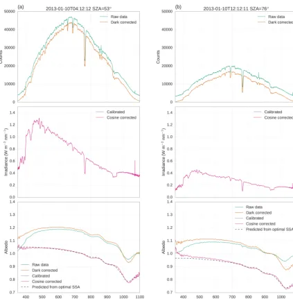
The effect of the processing steps is illustrated in this section for two acquisitions taken in contrasting solar conditions: a
first one at local noon on 10 January 2013 with the sun rela-tively high in the sky for Dome C (SZA=53◦) and a second one at 20:00 the same day (SZA=77◦). Figure 10a and b illustrate the contribution of each step (curves with different colors) for these acquisitions.
The first step (dark correction) is shown in Fig. 10 (or-ange). It removes the overall offset that is clearly visible in the raw data at wavelengths where the CMOS sensor has little sensitivity (under 350 nm and around 1100 nm). This correction has a positive side effect as it also reduces the small peaks due to damaged pixels like at 862 and 1069 nm. With the aging of the spectrometer, the number of such pix-els tended to increase (data not shown), but they remain iso-lated and the correction is efficient. The albedo is affected by this correction especially near the margins of the spectrum where the sensitivity of the CMOS sensor fades. Because both the incident and reflected spectra are equally affected by the same offset value, the albedo calculated with uncor-rected data tends to 1 near the margins. Since clean snow albedo is expected to tend to about 0.98–0.99 in the green and blue wavelengths, uncorrected data may appear better, but it is an artifact and the offset really needs to be corrected. At the other side of the spectrum, in the near-infrared, the cor-rection significantly changes the shape of the absorption fea-ture around 1030 nm by lowering the local minimum which has a huge impact on the SSA estimation. Applying the SSA retrieval algorithm on the albedo spectra, we find that SSA drops from 53 to 41 m2kg−1after the correction for the noon acquisition and from 61 to 24 m2kg−1for the evening one. These huge differences highlight the necessity of this correc-tion.
To evaluate this processing step within the modeling framework developed in Sect. 2.3.1, we consider typical val-ues of the noon acquisition: the spectrum has an amplitude of nearly 50 000 and the dark current (offset) is around 3800. We further assume that this offset can estimated with an accu-racy of 10 % (pessimistic estimate for illustration), which re-sults ind0=0.8 %. Figure 11 shows the perfect albedo (black curve) calculated for a true SSA of 50 m2kg−1and the per-turbed albedo (green curve) withd0= +0.8 %. Despite the small difference between the spectra, the estimated SSA is 55.4 m2kg−1, which corresponds to a relatively large over-estimation of 10 % but remains under our criteria of 15 %. Considering that the dark current can be usually estimated by much better than 10 %, the impact on the SSA is always minor.
The next processing step (stray light correction) is not shown because it has a negligible effect. Nevertheless, it is worth noting that we assume the stray light effect to be uni-form on all the pixels of the CMOS sensor. If this is not the case, the correction of the stray light would require a more complex method and the evaluation of the error proposed here would be only a lower bound of the error.
Figure 10.Incident spectrum and albedo at different stages of the processing for 10 January 2013 (left) at 12:12 LT and (right) at 20:12 LT. Raw data (green) are first corrected for the dark current and stray light (orange) then calibrated (violet) and last corrected for imperfect collectors (pink). The theoretical spectrum that fits the fully corrected spectrum (pink) is shown in black.
change the shape of the spectra. The most visible change on the radiance is mainly due to the absolute calibration be-cause it takes into account the sensitivity of the spectrom-eter. As expected for a silicon-based sensor, the correction increases the signal in the blue and near-infrared relative to the yellow and red. Nevertheless, the absolute calibration is not important for the albedo as explained before. The dif-ference on the albedo graphs before (orange curve) and af-ter (violet curve) the calibrations is only due to the cross-calibration step between the downward- and upward-looking channels and corresponds to a scaling that linearly decreases from 0.95 in the blue to 0.85 in the near-infrared. Because of this wavelength dependence, the SSA estimation is strongly affected, values decrease from 41 m2kg−1before correction
to 36 m2kg−1after for the noon acquisition and from 24 to 20 m2kg−1 for the evening one. In the theory presented in Sect. 2.3.2 this corresponds to approximatelyb=0.10. Us-ing Fig. 4, it means that the cross-calibration is definitely re-quired to reach the 15 % accuracy of SSA. If we assume that the correction is precise within 10 % (for instance because of the limited reproducibility of the experiment to determine the reference spectra) it leads to a residual trend ofb≈0.01 which is weak enough to reach the 15 % accuracy. In addi-tion, it is worth noting that this correction is constant over the whole time series and has therefore no impact on the relative temporal variations of SSA.
(mid-Figure 11. Simulations of albedo spectrum for a SZA=60◦. A perfect albedo spectrum for an homogeneous snowpack with SSA of 50 m2kg−1(black) is perturbed (green) by adding an offset of
d0=0.8 % of the maximum incident irradiance to the incident and reflected irradiance. It is used as an observation to estimate SSA using the range 700–1050 nm. The estimated spectrum is shown in orange (long dash).
dle graph) whatever the acquisition hour. The impact is also apparently moderate on the albedo (bottom graph). The cor-rection factor ranges from 0.98 in the blue to 0.99 in the near-infrared at noon and 1.00 to 1.07 at 8 p.m. Even though these values are weak, the correction successfully removes the de-creasing trend in the shorter wavelengths of the visible (400 to 600 nm) that affects the evening acquisition. Albedo mea-surements by Nicolaus et al. (2010) show a similar artifact. Such a trend is visible throughout the time series at large SZA and the collector response correction usually performs well by recovering a nearly constant value as expected.
Regarding SSA estimation, the correction has a little im-pact for the noon acquisition (36.7 and 36.2 m2kg−1, respec-tively, before and after the correction) as expected. In con-trast, for the evening acquisition the SSA estimate increases from 20 to 35 m2kg−1, the latter being close to the value at noon. This clearly shows that the correction of the collector response is crucial. The theoretical spectrum that fits the fully corrected spectrum is shown in black in Fig. 10. The differ-ences between the fit and the observation are small; we can note a slight overestimation at 800 nm and underestimation at 970 nm, both of which are very likely due to a small error in the refractive index of the ice already pointed out in other studies (e.g., Carmagnola et al., 2013). In contrast, the over-estimation at 1030 nm is more likely an error in the observa-tions resulting from the low sensitivity of the spectrometer in this wavelength range.
3.5 Stability
Before deriving albedo and SSA over long periods of time, it is important to assess the overall stability of the instrument.
The leveling is a first and important parameter. It was care-fully done at the installation of Autosolexs in December 2012 within the uncertainty allowed by spirit level (about 0.2◦) but could have degraded. Nevertheless, in December 2015, new measurements with an electronic devices yielded insignifi-cant movement of the structure.
The radiometric stability is another parameter. The sea-sonal variations of downwelling irradiance are plotted in Fig. 12 for the two heads and for the three summer seasons. The irradiance is integrated between 400 and 1000 nm and averaged between 10:00 and 14:00 h (local time). These data include all weather conditions. Overall, there is a good year-to-year agreement. For instance, the irradiance observed by the head 1 during the 30 days after the solstice (period in common for the three seasons) has increased by +0.5 and +4.2 % the second and third years with respect to the first one. These values become−0.5 %, and +3.0 %, respectively, for the head 2, which is relatively small for an unattended in-strument and considering that these values include the inter-annual variability of cloudiness. Only the third season shows a significant increase (around 4–5 %), which is unexplained.
4 Observations, interpretation, and comparison This section presents the 3-year time series of retrieved SSA and provides an analysis of its quality and information con-tent.
4.1 Diurnal cycle of SSA
The SSA estimated over the course of a day for each head is depicted in Fig. 13a for 10 January 2013 as a function of the local hour and the corresponding SZA. Gray symbols rep-resent data rejected for one of the three reasons: presence of clouds, excessive chromatic aberration, orAoutside the range 0.9–1.1.
On this particular day clouds were detected only at 03:25 and after 21:00 but the detection may not be reliable at high SZA because of the simplistic approach used to scale the ref-erence spectrum to a given SZA (Sect. 3.3). The other cases of rejection are equally due to the two other criteria. The other cases of rejection are equally due to the two other cri-teria and usually occur when the SZA is higher than 70◦. The SSA of rejected acquisitions is often close to valid ones, which could indicate that our criteria are too conservative. However, some data at very high SZA are not rejected al-though we believe they should have been. For this reason, we let the criteria be conservative and even discarded acqui-sitions at SZA higher than 75◦in the following.
Figure 12. Temporal variations of downwelling irradiance mea-sured by the two heads, averaged every day between 12:00 and 14:00 LT and averaged between 500 and 600 nm for three summer seasons (the year indicated in the legend refers to the month of De-cember).
40 m2kg−1for head 2. Root mean squared variations are, re-spectively, 0.9 and 2.6 m2kg−1, which is well under the 15 % target accuracy. The mean difference between both heads is 2.6 m2kg−1. The nearly perfect symmetry around noon sug-gests that these variations are not real but are caused by SZA-dependent errors due to either uncorrected artifacts in the ob-servations or limitation of the theoretical model used for the estimation.
The diurnal cycle is shown in Fig. 13b (1 March 2013). The SSA is much higher than in the previous case and the number of hours with SZA lower than 75◦is more limited. In addition, more data are rejected, mostly because of the chro-matic aberration. Altogether, the valid values range between 53 and 74 m2kg−1, representing a large amplitude of 30 %. The standard deviation is about 3.5 m2kg−1for both heads, that is, 10 % for a ±1σ variation. It was impossible to de-termine whether these variations are real or result from mea-surement and retrieval errors. These variations must therefore be interpreted as an upper bound estimate of the uncertainty of the retrieved SSA.
4.2 Statistical characteristics of the seasonal variations The seasonal variations of SSA estimated from the two heads over three summers (December 2012 to March 2015) are shown in Fig. 14 (Picard et al., 2016). The daily mean of valid data is plotted in color and each individual valid datum is shown in blue in the background to give an idea of the di-urnal variability (or maybe residual error). In this paper, we perform a quality assessment of this series. The interpreta-tion of the geophysical features is addressed in Libois et al. (2015).
Figure 13.Diurnal variations of estimated SSA for 10 January 2013 (top) and 1 March 2013 (bottom) for the two heads. Gray symbols show data rejected by the quality checks.
Figure 14.Seasonal variations of SSA for three summers since De-cember 2012 for the two heads. The blue dots show individual valid data (both heads) and the symbols show the daily mean of valid data for each head.
very little impact, the difference ranges between −1.0 and +1.5 m2kg−1depending on the season and head.
The two heads give very close values (within the daily range of variation) for some periods while significant differ-ences are observed for others usually in the spring (October 2013 and most remarkably October–November 2014) and in the fall (March 2013 and 2014). If we consider December– January to assess the statistics, we find the difference be-tween heads 1 and 2 to be −2.7, 1.0, and 0.0 m2kg−1 on average and 3.2, 2.4, and 2.2 m2kg−1root mean square, re-spectively, for the three seasons. This rules out any
signif-icant bias between the two heads which could have come from issues with the cross-calibration, the only processing step that uses different data depending on the head. This also indicates that the seasonal stability of the instrument and pro-cessing is of the same order as the diurnal standard deviation (Sect. 4.1). Conversely, it means that the difference observed during some periods might originate from the difference of SSA between the footprints of the two heads (Sect. 4.3).
Altogether these results indicate that the precision is much better than the targeted 15 % which ensures that the seasonal variations can be interpreted as a geophysical signal (Libois et al., 2015). In contrast, the absolute accuracy remains un-known as it mostly depends on the validity of the model in general and the choice of the parameter values (shape factors, assumption of a flat surface, etc.).
4.3 Horizontal variability between both heads
The two heads located 2 m apart show very similar variations most of the time (Fig. 14) and agree on the overall seasonal decrease from values higher than 60–80 m2kg−1 in Octo-ber to a minimum around 25 m2kg−1occurring in January and/or February. However, they also significantly differ dur-ing some periods. The heads bedur-ing at 2 m above the surface and accounting for the cosine weighting of the collector, we estimate that 50 % of the received signal comes from a disk of 2 m in radius (12 m2in surface area) and 75 % from a disk of 3.5 m in radius (38 m2). Despite the proximity and a slight partial overlap of the footprints, differences between the two heads can be particularly marked as in Spring 2014. We could invoke the fact that snow accumulation is irregular at Dome C (Petit et al., 1982; Libois et al., 2014a), leading to irregu-lar deposition on the surface. However, this argument is not compatible with the absence of difference observed during the summers although several precipitation events occurred and had a clear effect on the observed SSA (Libois et al., 2015) but did not lead to differences between both heads.
In spring 2014, the large and persistent difference could be ascribed to the presence of an erosional feature under head 1 (Fig. 5) and a wind-form feature (elongated dune) under head 2. The latter could be composed of recently deposited snow while the former feature sastrugi and older snow layers emerging on the surface. Nevertheless, this interpretation is subject to caution because visible photography is insensitive to SSA, as evidenced by the resemblance of the two pictures taken 12 October and 27 November despite a 3-fold decrease of the SSA.
and those areas may have different SSA. The direct effect of the roughness could also affect the symmetry of the diurnal cycle when the surface is rough but assessing the spectral ef-fect of the roughness is difficult and beyond the scope of this study.
4.4 Comparison with ASSSAP
Manual measurements of superficial snow SSA were taken with ASSSAP (Arnaud et al., 2011; Libois et al., 2015), a device using reflectance at 1310 nm to estimate SSA using similar theory as used here. For these measurements, we fol-lowed a specific protocol that takes care to preserve the sur-face and prevent post-sampling transformation of the snow. More than five manual measurements were taken every day in a site located approximately 1 km from Autosolexs. The sampling strategy was not random but aimed at covering the variety of different surface facies identified by the operator. It implies that the average of the values may differ from the true areal average of SSA when the spread of SSA is large.
Figure 15 shows individual manual measurements taken during the 2013–2014 season with ASSSAP, along with Au-tosolexs SSA time series (average of the two heads). Fig-ure 15 clearly shows that most manual measFig-urements signifi-cantly differ from the SSA estimated from Autosolexs. How-ever, the lowest values seem to agree with Autosolexs during the first part of the season, until about 8 January. After this, the spread of manual measurements is significantly reduced and despite higher values of SSA with ASSSAP, the temporal variations are correlated with those of Autosolexs.
This comparison clearly demonstrates that the SSA re-trieved in different wavelength ranges differ, which we at-tribute to strong heterogeneity of SSA between the upper-most 5 mm and 1 cm according to the calculation presented in Sect. 2.2.
The large difference in the first part of the season can be attributed to the frequent blowing snow events occurring dur-ing this period but the difference persists after 8 January de-spite calmer conditions. This persistence of large difference of SSA over a small vertical distance is not well understood (Gallet et al., 2011). Clear-sky precipitation (a.k.a. diamond dust) is a possible candidate but snow evolution simulation performed by Libois et al. (2015) uses ERA-Interim as in-put. The reanalysis successfully forecasts the precipitation events which leads to marked rises of SSA (Fig. 14) but does not include diamond dust. Since the simulation agrees with the SSA observations, this indicates that diamond dust is not required in the model to get a sustained high surface SSA on the surface. We conclude that a significant SSA gradient in the first uppermost centimeters exists with SSA possibly exceeding 100 m2kg−1on the very surface and that this gra-dient persists over long periods, even during periods without precipitation and blowing snow.
Figure 15.Time series of daily mean SSA averaged for the two heads of Autosolexs (black line) and manual measurements taken using ASSSAP (red dots). Both instruments have different vertical sensitivity as illustrated in Fig. 1.
5 Discussions and Conclusion
With a 16-channel optical switch, it is technically possible to set up seven measurement heads. (3) The leveling of the head should be and remain horizontal not only for albedo, which has been highlighted by numerous authors (e.g., Bo-gren et al., 2016), but also for SSA retrieval. Under typical polar summer conditions or in winter in the midlatitudes, we estimate the leveling must be better than 1◦to get the noon acquisition accurate enough to retrieve SSA with an accuracy of 15 %. Maintaining automatically the leveling and measur-ing the inclination at low temperature is challengmeasur-ing. (4) De-signing good light collectors and correcting for their imper-fect response is necessary for SZA above 60◦and becomes more and more critical above 70◦. The determination of the atmospheric diffuse/direct ratio and cloud mask deserves fur-ther work compared to what has been implemented here. Us-ing the measured incident spectrum to infer the actual ratio is an avenue. (5) Filtering data based on the difference between observed and estimated albedo in the visible range discards data subject to any artifact that produces excessive chromatic aberration. The approach developed here does not require high spectral resolution data; it can be applied to multi-band radiometers like those carried by satellites. However, it re-quires some assumptions like negligible impurity content and could interfere with the atmospheric correction often based on the blue channels for space-borne sensors.
Part of the difficulties addressed in this study arises from the weak sensitivity of the SSA–reflectance relationship at wavelengths under 1 µm, especially for the high SSA encoun-tered at Dome C (50 m2kg−1 and higher) (Domine et al., 2006; Gallet et al., 2009). Extending the present instrument further in the infrared seems attractive because the sensitivity to SSA is greater so that larger error on the albedo measure-ment would be acceptable for a similar target accuracy of SSA. However, it comes at a price. Building light collectors with a good angular response is increasingly challenging at longer wavelengths due to the decreasing scattering. The bal-ance between theoretically more sensitive wavelengths and increasing chromatic aberrations needs to be weighted.
The influence of the surface roughness on the albedo and estimated SSA also deserves further work. Warren et al. (1998) explained that “introducing roughness will cause no change to the albedo of a surface whose albedo is 0.0 or 1.0. The greatest effect is for intermediate values of albedo; in the case of snow, this means near-infrared wavelength”, which implies that roughness change tends to reduce albedo in the 1030 nm absorption feature more than at shorter wave-lengths. This implies that our algorithm, by assuming a flat interface, would underestimate the SSA over rough surfaces. Moreover, with measurement heads only 2 m above the sur-face, the scale of the measurements and that of the rough-nesses are of the same order resulting in a more complex problem than that considered in modeling studies (Leroux and Fily, 1998). Spatial survey of albedo and SSA variations could be used to evaluate this effect. The anisotropy of the roughness and the slope of the terrain (relevant to
mountain-ous regions only) are expected to introduce a spurimountain-ous diurnal cycle and need to be considered in the future as well.
The present study, by retrieving 3-year time series of SSA, confirms the general coarsening of snow grains during the summer observed in several studies (Jin et al., 2008; Picard et al., 2012) and recently shown to be predicable by snow metamorphism modeling (Libois et al., 2015). However, de-spite its length, it features relatively little interannual vari-ations compared to that observed by satellite and provides little evidence yet of modulation of the grain size by pre-cipitation at the seasonal timescale as hypothesized by Pi-card et al. (2012). An important perspective of this work is to maintain Autosolexs at Dome C and to develop the installa-tion of ground-based spectral radiometers in Antarctica.
6 Data availability
Processed spectral albedo time series is available through Pangea database (doi:10.1594/PANGAEA.860945, Picard et al., 2016).
Author contributions. G. Picard and L. Arnaud developed and built Autosolexs, and L. Arnaud and Q. Libois deployed it at Dome C and performed the calibration experiments. G. Verin performed the collector characterization. M. Dumont conducted the atmospheric simulations. G. Picard and Q. Libois developed the retrieval algo-rithm and prepared the manuscript with contributions from the other authors.
Acknowledgements. This study was supported by the ANR program 1-JS56-005-01 MONISNOW. The authors acknowledge the French Polar Institute (IPEV) for the financial and logistic support at Concordia station in Antarctica through the NIVO program. This work has also been supported by a grant from OSUG@2020 (investissement d’avenir – ANR10 LABX56). We thank the IPEV winter-over staff at Concordia for monitoring our snow instruments, including Autosolexs.
Edited by: R. Brown
References
Aoki, T., Aoki, T., Fukabori, M., Hachikubo, A., Tachibana, Y., and Nishio, F.: Effects of snow physical parameters on spectral albedo and bidirectional reflectance of snow surface, J. Geophys. Res., 105, 10219–10236, doi:10.1029/1999JD901122, 2000. Arnaud, L., Picard, G., Champollion, N., Domine, F., Gallet, J.,
Bogren, W. S., Burkhart, J. F., and Kylling, A.: Tilt error in cryospheric surface radiation measurements at high latitudes: a model study, The Cryosphere, 10, 613–622, doi:10.5194/tc-10-613-2016, 2016.
Carmagnola, C. M., Domine, F., Dumont, M., Wright, P., Strellis, B., Bergin, M., Dibb, J., Picard, G., Libois, Q., Arnaud, L., and Morin, S.: Snow spectral albedo at Summit, Greenland: measure-ments and numerical simulations based on physical and chemi-cal properties of the snowpack, The Cryosphere, 7, 1139–1160, doi:10.5194/tc-7-1139-2013, 2013.
Curry, J. A., Schramm, J. L., and Ebert, E. E.: Sea Ice-Albedo Climate Feedback Mechanism, J. Climate, 8, 240–247, doi:10.1175/1520-0442(1995)008<0240:siacfm>2.0.co;2, 1995. Domine, F., Salvatori, R., Legagneux, L., Salzano, R., Fily, M., and Casacchia, R.: Correlation between the specific surface area and the short wave infrared (SWIR) reflectance of snow, Cold Reg. Sci. Technol., 46, 60–68, doi:10.1016/j.coldregions.2006.06.002, 2006.
Dumont, M., Brissaud, O., Picard, G., Schmitt, B., Gallet, J.-C., and Arnaud, Y.: High-accuracy measurements of snow Bidi-rectional Reflectance Distribution Function at visible and NIR wavelengths – comparison with modelling results, Atmos. Chem. Phys., 10, 2507–2520, doi:10.5194/acp-10-2507-2010, 2010. Ettema, J., van den Broeke, M. R., van Meijgaard, E., and van de
Berg, W. J.: Climate of the Greenland ice sheet using a high-resolution climate model – Part 2: Near-surface climate and en-ergy balance, The Cryosphere, 4, 529–544, doi:10.5194/tc-4-529-2010, 2010.
Fierz, C., Armstrong, R. L., Durand, Y., Etchevers, P., Greene, E., McClung, D. M., Nishimura, K., Satyawali, P. K., and Sokratov, S. A.: The international classification for seasonal snow on the ground, UNESCO/IHP, 2009.
France, J. L., King, M. D., Frey, M. M., Erbland, J., Picard, G., Preunkert, S., MacArthur, A., and Savarino, J.: Snow optical properties at Dome C (Concordia), Antarctica; implications for snow emissions and snow chemistry of reactive nitrogen, At-mos. Chem. Phys., 11, 9787–9801, doi:10.5194/acp-11-9787-2011, 2011.
Gallet, J.-C., Domine, F., Zender, C. S., and Picard, G.: Measument of the specific surface area of snow using infrared re-flectance in an integrating sphere at 1310 and 1550 nm, The Cryosphere, 3, 167–182, doi:10.5194/tc-3-167-2009, 2009. Gallet, J.-C., Domine, F., Arnaud, L., Picard, G., and Savarino, J.:
Vertical profile of the specific surface area and density of the snow at Dome C and on a transect to Dumont D’Urville, Antarc-tica – albedo calculations and comparison to remote sensing products, The Cryosphere, 5, 631–649, doi:10.5194/tc-5-631-2011, 2011.
Gardner, A. S. and Sharp, M. J.: A review of snow and ice albedo and the development of a new physically based broadband albedo parameterization, J. Geophys. Res., 115, doi:10.1029/2009jf001444, 2010.
Goelles, T., Bøggild, C. E., and Greve, R.: Ice sheet mass loss caused by dust and black carbon accumulation, The Cryosphere, 9, 1845–1856, doi:10.5194/tc-9-1845-2015, 2015.
Grenfell, T. C., Warren, S. G., and Mullen, P. C.: Reflection of solar radiation by the Antarctic snow surface at ultraviolet, visible, and near-infrared wavelengths, J. Geophys. Res., 99, 18669–18684, doi:10.1029/94JD01484, 1994.
Grenfell, T. C. and Warren, S. G.: Representation of a nonspherical ice particle by a collection of independent spheres for scatter-ing and absorption of radiation, J. Geophys. Res., 104, 31697– 31710, doi:10.1029/1999JD900496, 1999.
Hudson, S. R., Warren, S. G., Brandt, R. E., Grenfell, T. C., and Six, D.: Spectral bidirectional reflectance of Antarctic snow: Measurements and parameterization, J. Geophys. Res., 111, doi:10.1029/2006jd007290, 2006.
Hudson, S. R. and Warren, S. G.: An explanation for the effect of clouds over snow on the top-of-atmosphere bidirectional re-flectance, J. Geophys. Res., 112, doi:10.1029/2007JD008541, 2007.
Jin, Z., Charlock, T. P., Yang, P., Xie, Y., and Miller, W.: Snow op-tical properties for different particle shapes with application to snow grain size retrieval and MODIS/CERES radiance compar-ison over Antarctica, Remote Sens. Environ., 112, 3563–3581, 2008.
Kantzas, E. P., McGonigle, A. J. S., and Bryant, R. G.: Comparison of Low Cost Miniature Spectrometers for Vol-canic SO2 Emission Measurements, Sensors, 9, 3256–3268,
doi:10.3390/s90503256, 2009.
Kokhanovsky, A. A. and Zege, E. P.: Scattering optics of snow, Appl. Optics, 43, 1589–1602, 2004.
Kuchiki, K., Aoki, T., Niwano, M., Motoyoshi, H., and Iwabuchi, H.: Effect of sastrugi on snow bidirectional reflectance and its application to MODIS data, J. Geophys. Res., 116, doi:10.1029/2011jd016070, 2011.
Leroux, C. and Fily, M.: Modeling the effect of sastrugi on snow re-flectance, J. Geophys. Res., 103, 25779, doi:10.1029/98je00558, 1998.
Libois, Q., Picard, G., France, J. L., Arnaud, L., Dumont, M., Car-magnola, C. M., and King, M. D.: Influence of grain shape on light penetration in snow, The Cryosphere, 7, 1803–1818, doi:10.5194/tc-7-1803-2013, 2013.
Libois, Q., Picard, G., Arnaud, L., Morin, S., and Brun, E.: Mod-eling the impact of snow drift on the decameter-scale variability of snow properties on the Antarctic Plateau, J. Geophys. Res.-Atmos., 119, 11662–11681, doi:10.1002/2014jd022361, 2014a. Libois, Q., Picard, G., Dumont, M., Arnaud, L., Sergent, C.,
Pougatch, E., Sudul, M., and Vial, D.: Experimental determi-nation of the absorption enhancement parameter of snow, J. Glaciol., 60, 714–724, doi:10.3189/2014jog14j015, 2014b. Libois, Q., Picard, G., Arnaud, L., Dumont, M., Lafaysse, M.,
Morin, S., and Lefebvre, E.: Summertime evolution of snow spe-cific surface area close to the surface on the Antarctic Plateau, The Cryosphere, 9, 2383–2398, doi:10.5194/tc-9-2383-2015, 2015.
Macke, A. and Mishchenko, M. I.: Applicability of regular particle shapes in light scattering calculations for atmospheric ice parti-cles, Appl. Optics, 35, 4291, doi:10.1364/AO.35.004291, 1996. Marks, A., Fragiacomo, C., MacArthur, A., Zibordi, G., Fox, N.,
and King, M. D.: Characterisation of the HDRF (as a proxy for BRDF) of snow surfaces at Dome C, Antarctica, for the inter-calibration and inter-comparison of satellite optical data, Remote Sens. Environ., 158, 407–416, doi:10.1016/j.rse.2014.11.013, 2015.