www.ocean-sci.net/6/679/2010/ doi:10.5194/os-6-679-2010
© Author(s) 2010. CC Attribution 3.0 License.
Ocean Science
Mixed layer sub-mesoscale parameterization – Part 1:
Derivation and assessment
V. M. Canuto1,2and M. S. Dubovikov1,3
1NASA, Goddard Institute for Space Studies, New York, NY, 10025, USA 2Dept. Appl. Math. and Phys., Columbia University, New York, NY, 10027, USA 3Center for Clim. Systems Res., Columbia University, New York, NY, 10025, USA
Received: 7 August 2009 – Published in Ocean Sci. Discuss.: 17 September 2009 Revised: 9 June 2010 – Accepted: 28 June 2010 – Published: 16 July 2010
Abstract. Several studies have shown that sub-mesoscales (SM∼1km horizontal scale) play an important role in mixed layer dynamics. In particular, high resolution simulations have shown that in the case of strong down-front wind, the re-stratification induced by the SM is of the same order of the de-stratification induced by small scale turbulence, as well as of that induced by the Ekman velocity. These studies have further concluded that it has become necessary to include SM in ocean global circulation models (OGCMs), especially those used in climate studies.
The goal of our work is to derive and assess an analytic parameterization of the vertical tracer flux under baroclinic instabilities and wind of arbitrary directions and strength. To achieve this goal, we have divided the problem into two parts: first, in this work we derive and assess a parameterization of the SM vertical flux of an arbitrary tracer for ocean codes that resolve mesoscales, M, but not sub-mesoscales, SM. In Part 2, presented elsewhere, we have used the results of this work to derive a parameterization of SM fluxes for ocean codes that do not resolve either M or SM.
To carry out the first part of our work, we solve the SM dy-namic equations including the non-linear terms for which we employ a closure developed and assessed in previous work. We present a detailed analysis for down-front and up-front winds with the following results:
(a) down-front wind (blowing in the direction of the sur-face geostrophic velocity) is the most favorable condition for generating vigorous SM eddies; the de-stratifying effect of the mean flow and re-stratifying effect of SM almost cancel each other out,
Correspondence to: V. M. Canuto ([email protected])
(b) in the up-front wind case (blowing in the direction op-posite to the surface geostrophic velocity), strong winds pre-vents the SM generation while weak winds hinder the pro-cess but the eddies amplify the re-stratifying effect of the mean velocity,
(c) wind orthogonal to the geostrophic velocity. In this case, which was not considered in numerical simulations, we show that when the wind direction coincides with that of the horizontal buoyancy gradient, SM eddies are generated and their re-stratifying effect partly cancels the de-stratifying ef-fect of the mean velocity. The case when wind direction is opposite to that of the horizontal buoyancy gradient, is anal-ogous to the case of up-front winds.
In conclusion, the new multifaceted implications on the mixed layer stratification caused by the interplay of both strength and directions of the wind in relation to the buoy-ancy gradient disclosed by high resolution simulations have been reproduced by the present model.
The present results can be used in OGCMs that resolve M but not SM.
1 Introduction
Recently, there has been a considerable interest in sub-mesoscales (SM) which are oceanic structures with sizes O(1 km) and a life time of the order of days. If one considers that the highest resolution O(1/100)in stand-alone OGCMs (ocean global circulation models) can represent structures of about 10 km which is 10 times larger than SM sizes and that OGCMs employed in thousand years runs for climate studies have in general a 10resolution (corresponding to structures 100 times larger than SM sizes), it seems clear that a good deal of important physical processes have thus far gone un-represented in many OGCMs.
characterized by a small Rossby number Ro=ζ /f1 (where ζ and f are the relative and planetary vorticities respec-tively), mixed layer SM are characterized by Ro∼1 (Thomas et al., 2008). Thus, the dynamics of M and SM are quite dif-ferent and so are the final results for the fluxes of interest. For this reason, the parameterizations for M that were suggested for the deep ocean cannot be extrapolated to describe SM in the mixed layer and a new parameterization is required.
Most of the present knowledge about mixed layer SM comes from high resolution numerical simulations (Levy et al., 2001; Thomas and Lee, 2005; Mahadevan, 2006; Ma-hadevan and Tandon, 2006; Klein et al., 2008; Thomas et al., 2008; Capet et al., 2008, C8; Levy et al., 2010; Mahadevan et al., 2010, MTF). These studies have revealed many inter-esting features of SM, e.g., their contribution to the vertical mixing of buoyancy and tracers in the upper ocean. Among the most salient effects of SM on global ocean properties is the well documented tendency to re-stratify the mixed layer (Spall, 1995; Nurser and Zhang, 2000; C8; MTF). The effect of SM on deep convection has been recently demonstrated by Levy et al. (2009, Fig. 9) who point out a better agree-ment with the new mixed layer data by Boyer Montegut et al. (2004) south of the WBC (Western Boundary Current). Even in non-convective regimes, one can expect a signifi-cant cancellation between SM and small scale fluxes lead-ing to the mixed layer re-stratification (e.g., C8, Fig. 12; Klein et al., 2008); Hosegood et al. (2008) estimated that SM contribute up to 40% of the re-stratification process. In addition, as noted by Lapeyre et al. (2006) and Klein et al. (2008), the surface layers re-stratification is compensated by de-stratification of the ocean interior pointing to an in-teresting dynamical connection between surface and interior processes. Another important effect of SM concerns the lo-cation of the WBC that is shifted south by 40 and whose off shore extension penetrates further to the east, in better agreement with observations (Levy et al., 2009). An earlier study by Treguier et al. (2005), who found a significant in-crease (from∼30 Sv to∼70 Sv) in the barotropic transport in the Gulf Stream when moving from 10to 1/60resolution, was recently confirmed and the inclusion of SM further in-creased the transport by∼50 Sv. Finally, the structure of the MOC (meridional overturning circulation) was also signifi-cantly affected by SM not so much in its intensity as to its location (Levy et al., 2009, Fig. 12).
This brief summary of some of the results of very high resolution (1/540,∼2 km) regional studies highlights the im-portance of SM and thus the question arises as to how much of SM physics is actually accounted for by global OGCMs. Even today’s highest resolution global ocean models∼1/100 (Maltrud and McClean, 2005; Sasaki et al., 2008) are not able to capture the SM field and much less are in the position to do so the OGCMs coupled to an atmospheric model used in climate studies where the resolution is O(10) but gener-ally lower. The significant global processes revealed in going from 10resolution (∼100 km) and 1/540resolution (∼2 km)
are presently absent in such global models especially in cli-mate studies. Therefore, a reliable parameterization of SM in terms of the resolved fields has become necessary to ensure the physical completeness of mixed layer mixing processes.
As MTF stressed, “parameterization of the circulation in-duced by SM eddies in the presence of wind forcing is required in climate models in order to simulate the re-stratification correctly”. To accomplish such a goal, a pa-rameterization: (1) must be valid for an arbitrary tracer since a model for buoyancy only is insufficient because it cannot describe an important ingredient such as CO2, (2) must
in-clude a wind of arbitrary direction and intensity since MTF have shown that its effect on SM fluxes is large and because forcing in future climates is likely to be quite different from today’s, (3) must reproduce simulation data and finally, (4) to be usable in climate codes, it must be expressed only in terms of resolved fields, that is, the parameterization must be aver-aged over mesoscale fields. No parameterization presently available satisfies these criteria.
We begin by considering the model independent dynamic equation for an arbitrary mean tracer1:
Dtτ + ∇H·FH+∂zFV =∂z(Kv∂zτ )+G (1a)
where the SM horizontal and vertical tracer fluxes are defined as follows:
FH≡u0τ0, FV≡w0τ0 (1b)
In Eqs. (1a,b), an overbar indicates averages over subme-soscales. To derive a parameterization for OGCMs that do not resolve either SM or M, one must further average the present results over the mesoscale fields, a problem we have studied elsewhere (Canuto and Dubovikov, 2010).
The method we employ to derive the SM parameteriza-tion is analytical and thus it can be followed and checked in detail. The final result for the vertical SM flux for an arbi-trary tracer under arbiarbi-trary buoyancy and wind conditions, is also expressed analytically. The model includes non-linear interactions. To obtain the desired results, one carries out three steps: first, one solves in Fourier space the SM dy-namic equations describing theu0,w0,τ0fields; second, one constructs the second-order correlation functionw0τ0 ink -space and third, one integrates the results over all wave vec-tors to obtain the fluxes in physical space in terms of the resolved fields, to be used in Eq. (1a). The procedure was first worked out for the linear case by Killworth (1997) and for the non-linear case by Canuto and Dubovikov (2005, 2006, CD5, 6). Though the dynamic equations describing the SM velocity and temperature fields are formally the same as those describing mixed layer mesoscales that were dis-cussed in Canuto et al. (2010), in the present case they must
1D
t=∂t+u·∇H+w∂z where (u, w) represent the mean flow,
small scale vertical mixing is represented by the first term in the right hand side of Eq. (1a) whereKvis the vertical diffusivity,G
be solved in the regime appropriate to SM, namely for a Rossby number Ro=ζ /f=O(1) rather than Ro1, as in the case of mesoscales. In addition, SM are trapped in the ML while mesoscales extend throughout the entire water column and form coherent structures (Provenzale, 1999).
The key difficulty in solving the SM dynamic equations is the presence of non-linear terms whose closure is expressed in Eq. (3a) below. Since the latter is a key ingredient of the present model and since the original derivation (Canuto and Dubovikov, 1997) is somewhat involved, in Appendices A and B we have attempted to find a way to present a more physical approach to Eq. (3a) with the goal of highlighting the physical rather than the technical features of Eq. (3a).
In addition to the derivation of the closure relations (Eq. 3a), there is the issue of the assessment of Eq. (3a) when applied to flows different than the present one so as to justify their use in the present context. Such an assess-ment was made using data from freely decaying flows, 2-D flows, rotating flows, unstably stratified flows, shear driven flows, DNS data, etc. and the results were in good agree-ment with the data (see Canuto et al., 1999 and references therein). Even so, we consider such an assessment necessary but not sufficient for the credibility of the parameterization of SM fluxes derived below. The additional requirement con-sists in assessing the model predictions against results from SM resolving simulations. A first simulation corresponds to a system forced only by baroclinic instabilities and no wind (Fox-Kemper et al., 2008, FFH) while a second one corre-sponds to a flow under realistic wind and buoyancy forcing (C8, 0.75 km resolution; MTF, 1 km resolution). They will be discussed in Sects. 5–7.
The following two conditions must be further satisfied by an SM parameterization: (a) it must reproduce existing data and (b) it must predict new features to be assessed when such data become available. In this context, it must be mentioned that our work was posted as an OS Discussions (Canuto and Dubovikov, 2009, CD9) before Dr. A. Mahadevan kindly sent us the MTF manuscript. Our model would have been falsified had its predictions turned out to be inconsistent with MTF data. However, the model predictions in CD9 not only did not contradict the simulation data, but called attention to the same qualitative SM effects as MTF did in their paper.
To make the SM parameterization usable in OGCMs, we looked for analytical solutions of the SM dynamic equations and to achieve that goal, we introduced the assumption that the fluxes are mostly contributed by their spectra in the vicin-ity of their maxima. Though this introduces errors of several tens of a percent, the advantages of obtaining analytic expres-sions for the vertical tracer flux in terms of resolved fields in the presence of both frontogenesis and Ekman pumping, was worth exploring. Another approximation which has helped us obtain analytical results follows from the assumption that the SM kinetic energyKSMexceedsKe=eu2/2 whereeuis the baroclinic component of the mean velocity (we call atten-tion to the fact thatKeis considerably smaller than the mean
kinetic energy), that is, the condition of applicability of the present treatment is predicated on the assumption:
e
KKSM (1c)
which we shall check several times in the following. Fur-thermore, following Killworth (2005), we adopt the approx-imation that due to the mixed layers strong mixing, one can neglectτzin the SM equations. Anticipating our main result,
the vertical flux that enters Eq. (1a) will be shown to have the following form:
∂zFV=u+S · ∇Hτ (1d)
whereu+S plays the role of a bolus velocity. Sinceτzis small,
one may make the analogy with the mesoscale bolus velocity more complete by adding to Eq. (1d) the termw+Sτz, where
w+S is found from the continuity condition∂zwS++∇H·u+S=0
(Killworth, 2005).
The organization of the paper is as follows. In sec.2 we discuss the dynamic equations for the SM fields in the ML and apply the turbulence closure model to the non-linear terms; in Sect. 3 we present the form of∂zFVandFVwhich
we derive in Appendix C; in Sect. 4 we derive the explicit form of the SM kinetic energyKSMin terms of the resolved
fields that, together with the results of the previous section, completes the problem of expressing∂zFV in terms of
re-solved fields in the presence of both frontogenesis and Ek-man pumping. In Sect. 5 we study the case of a strong wind when the Ekman velocity exceeds the geostrophic one. We shall show that when a strong wind blows in the direction of the geostrophic velocity or of∇Hb, it tends to de-stratify the mixed layer but at the same time it generates SM that tend to re-stratify the mixed layer. On the other hand, when the wind blows in directions opposite to geostrophic velocity or to ∇Hb, it re-stratifies the mixed layer, an effect that is strengthened by the re-stratifying effect of SM. In Sect. 6 we compare the model results with the data from the SM resolv-ing simulations of Capet et al. (2008). In Sect. 7 we compare the model results for the no-wind case. In Sect. 8, we present some conclusions.
2 Sub-mesoscales dynamic equations near the surface Consider an arbitrary tracer fieldτ and separate it into mean and fluctuating partsτ=τ+τ0. The dynamical equation for the SM tracer fieldτ0is obtained by subtracting the equation for the mean tracerτ from that of the total fieldτ. Since this procedure is well known and entails only algebraic steps with no physical assumptions, we cite only the final result (the notation is explained in footnote 1):
Dtτ0= −U0· ∇τ −QτH−QτV+∂z Kv∂zτ0 (2a)
QτH ≡ u0· ∇Hτ0−u0· ∇
Hτ0, QτV ≡w 0τ0
z−w0τ0z
must be noted that in Eqs. (2a) no closure has been used for the non-linear terms. Without the non-linear terms, Eqs. (2a) formally coincide with those describing mixed layer mesoscales tracer fields studied by Killworth (2005). The difference in representing M and SM lies in the scales over which the averages (represented by an overbar in Eqs. 2a), is taken: in the case of mesoscales, averages are over scales exceeding mesoscales while in the case of subme-soscales, averages are meant to be over scales smaller than mesoscales but larger than submesoscales. Furthermore, in describing mesoscales, one has Ro1 and Ri1, whereas in the case of sub-mesoscales, both Ro, Ri∼O(1). Following Killworth (2005), we neglect the terms containingτzandτ0z
in which case the first of Eqs. (2a) simplifies to:
∂tτ0+ ¯u· ∇Hτ0= −u0· ∇Hτ −QτH (2b)
Without the non-linear term, Eq. (2b) coincides with Eq. (2) of Killworth (2005) for the mesoscale buoyancy field. Within the same approximation, the equation for the horizontal SM velocity is given by:
∂tu0+ ¯u·∇Hu0+u0·∇Hu+fez×u0= −ρ−1∇Hp0−QuH (2c)
QuH ≡u0· ∇Hu0−u0· ∇
Hu0 (2d)
whereez is the unit vector along z axis. Next, we Fourier transform Eqs. (2b,c) in horizontal planes and time. Follow-ing Killworth (1997, 2005), we keep the same notationu0,τ0 for the submesoscale fields in the k−ωspace and assume that when Eqs. (2b,c) are Fourier transformed, the mean fieldsu
and∇Hτare constant in time and horizontal coordinates. We thus obtain:
i(k· ¯u−ω)τ0= −u0· ∇Hτ −QτH
i(k· ¯u−ω)u0= −u0· ∇Hu−fezxu0−QuH−ikρ −1p0
∂zw0= − ∇H ·u0= −ik·u0 (2e)
where we have added the continuity equation that provides the z-derivative ofw0. We recall that τ0, u0 and the non-linear terms are functions of the horizontal wave vector and frequency (k,ω) and z, whileu¯ is a function of z only and ∇Hτ is z independent.
Equations (2e) form a closed system whose solution pro-vides the necessary ingredients to construct the vertical flux (Eq. 1b) provided one has a closure for the non-linear terms, a problem discussed in Appendices A and B with the result that, in the vicinity ofk=k0where the SM energy spectrum
E(k) has its maximum, the non-linear termsQH have the
following forms:
QτH(k, ω)=χ τ0(k, ω), QuH(k, ω)=χ u0(k, ω), (3a)
χ=k0USM, KSM=
1 2U
2 SM
where the scale`=k−01 may be interpreted as the SM hori-zontal length scale. As it was shown in detail in CD5,k0is
obtained from the solution of the eigenvalue problem which is derived from the eddy dynamical equations (Eq. 2e). In the limit of a strong non-linearity represented by:
KSM>K,e Ke= 1 2eu
2 (3b)
whereKeis the kinetic energy of the baroclinic component of the mean velocity (defined in Eq. 4b), the solution of the eigenvalue problem yields the following result:
k−01=`≈rS=π−1(N/|f|)h (3c)
whererSis the Rossby deformation radius of the mixed layer
(ML) of depth h and where N is the buoyancy frequency in the ML. Relation (Eq. 3c) is in qualitative agreement with other evaluations of the submesoscale length scale discussed in the literature (Boccaletti et al., 2007; Thomas et al., 2008; Fox-Kemper and Ferrari, 2008). In Fig. 9 of Fox-Kemper et al. (2008), the authors, using simulation data, plot SM length scales defined using different variables and in unit of the Stone length scale which is of the order of the deforma-tion radius.
Equation (2e) together with Eq. (3a), represent a stochastic Langevin equation which has played a major role in turbu-lence modeling studies (Kraichnan, 1971; Leith, 1971; Her-ring and Kraichnan, 1971; Chasnov, 1991). The advantage of the Langevin equation is that it is linear in the fluctuat-ing fields and thus allows one to compute second-order mo-ments while the original Eqs. (2b,c) are non-linear and do not allow an analytical computation of such correlation func-tions. The key problem is to find a model for the non-linear terms Q’s that leads to a Langevin equation whose corre-lation functions are sufficiently close to those of the orig-inal Eqs. (2b,c). This is the closure problem for the non-linear terms. In CD5, we used the closure (Eq. 3a) derived by Canuto and Dubovikov (1997) and solved the eigenvalue problem to which the mesoscale dynamic equations were shown to reduce. Closure (Eq. 3a) has a simple interpreta-tion within the mixing length approach. In fact, the first two relations are quite standard withχ−1being the characteristic time scale while the third relation containing the character-istic length scale (Eq. 3c) and velocity, is the only possible combination that leads to a time scale.
not coincide with the geostrophic velocity. In fact, Eq. (C12) shows that, using the third of Eq. (C6), in the limit (Eq. 1c),
uRcan be represented as follows:
uR= −
ikρ−1p0 1+1
2Ro2
, Ro=USM
|f|` (3d)
where Ro is the Rossby number andp0 is the SM pressure field. Thus, when treating mesoscales that are character-ized by small Ro, the first relation in Eq. (3d) reduces to the geostrophic relationuR→ug=−ikρ−1p0. On other hand,
since SM are characterized by Ro∼1, we must use the com-plete form of Eq. (C12). This is the reason why we have not calleduR the geostrophic component and the divergent
componentuD(Eq. C11) the a-geostrophic one.
3 Sub-mesoscale vertical tracer flux
Following the program we have outlined at the end of the previous section, in Appendix C we show how to express w0(k, ω)andτ0(k, ω)in terms of the SM horizontal velocity u0(k, ω)and of the resolved fields; that, in turn, allows us to express the spectrum ofFV≡w0τ0in terms of the SM energy
spectrum. Finally, integrating the spectra over all wavenum-bers, we obtain the following SM vertical tracer flux ∂zFV=u+S·∇Hτ , u+S=−
1+γ2
−1 eu−γ
f |f|ez×eu
(4a) where:
γ= rS|f| USM
= 1
Ro, eu=u−h −1
0 Z
−h
u(z)dz, (4b)
ez is the unit vertical vector and Ro is the Rossby number
defined in Eq. (3d). It is worth stressing that in the second relation in Eq. (4a), the second term in the square bracket is a vector: in fact, althoughez×euis a pseudo-vector (cross product of the vectorsezandeu), f is a pseudo-scalar which is the scalar product of the vectorezand the pseudo-vector
2and thus the product is a vector. The variableeumay be interpreted as the ML baroclinic part of the mean velocity. The parameterization (Eq. 4a,b) is obtained under condition (Eq. 1c) and can be obtained from Eq. (7a,b) of CD9 in the limit (Eq. 1c).
In Eq. (4a) the velocityu+S may be interpreted as the sub-mesoscale induced velocity which is a counterpart of the mesoscale induced velocity. As noted earlier, to make the analogy with the mesoscale induced velocity more complete and since in the mixed layerτz is small due to the strong
mixing, one may add to Eq. (4a) the termw+Sτz, wherewS+
is found from the continuity condition:
∂zwS++ ∇H ·u+S =0 (5)
The only variable in Eq. (4b) that is not yet parameterized is the SM kinetic energyKSM which we study in the next
section. Before doing so and for future reference, we next derive the explicit form of the vertical flux itself. Integrating Eq. (4a) over z with the boundary conditionFV(0)=0, we
ac-count for only the z-dependency ofeuwithin the mixed layer. Thus, we obtain:
FV= −κH· ∇Hτ (6a)
where the submesoscale diffusivity is given by:
κH=z
1+γ2 −1
bu−γ f |f|ez×bu
, (6b)
bu(z)=z −1
z Z
0 eudz
From Eq. (6b), one observes that at the bottom of the ML, z=−h, we have that:
bu(−h)=0, κH(−h)=0, FV(−h)=0 (6c) which is a good approximation since SM eddies hardly pen-etrate the bottom of the mixed layer (Boccaletti et al., 2007). We also have the additional relations:
bu(0)=0, κH(0)=0, FV(0)=0 (6d) 4 MS kinetic energy in terms of resolved fields
Assuming that the production ofKSMoccurs at scales`∼rs
and since the eddy kinetic energy equation shows that the vertical buoyancy fluxFVbacts as the source ofKSM, we
em-ploy the following relations:
KSM=C (rsPK)2/3, PK=<Fvb>≡h −1
0 Z
−h
dzFbV(z) (7a)
In the case of 3-D turbulence where kinetic energy cascades from large to small scales and a Kolmogorov spectrum sets in, the first relation in Eq. (7a) is simply the statement that production=dissipation with the former is defined in the sec-ond of Eq. (7a) while dissipation is represented by a Kol-mogorov form. In such a case, C=(3/2)Ko(1+A∗)where A∗>0 accounts for the contribution to KSM of the energy
spectrum atk<k0and Ko is the Kolmogorov constant whose
value ranges between 1.4–2.2. WithA∗=1, Ko=2, we have C=6. However, in the 2-D case of interest here, cascade of KSM to smaller scales does not take place. Instead, KSM
transforms into SM potential energy which we denote by WSM. Then, in the quasi-stationary case, the production of
KSM given in the second of Eq. (7a), approximately equals
the production ofWSM. Since the latter cascades to smaller
scales where is ultimately dissipated, we have:
whereC0 depends on the spectrum of WSM. If we further
denote by0SMthe ratio of the SM kinetic and potential
en-ergies, from Eq. (7b) we conclude that the first relation of Eq. (7a) is satisfied with:
C=0SMC0, 0SM=KSM/WSM (7c)
It is worth noticing that relations analogous to Eq. (7a,b) hold true for mesoscales as well with the proviso that the con-stantsC0, 0 and therefore C, are different for SM and M due to their different dynamics since, as already mentioned, SM are trapped in the ML while M form coherent struc-tures throughout the entire water column and thus entail the dynamics of the deep ocean. Using a mesoscale resolving simulation, Eq. (7a) was validated in more than 70 different mesoscale resolving simulations (Canuto et al., 2010). In the next sections, on the basis of Capet et al. (2008), we estimate thatC≈6. Even though at present we have determinedCon the basis of only one simulation by C8, we shall show be-low that the variable of interest to OGCMs, the tracer flux, is only weakly dependent onC. Substituting Eq. (6a,b) and rS=N h/π|f| into Eq. (7d), we obtain the following
alge-braic equation forKSM:
KSM3/2=C3/2(1+γ2)−1hrs(V −γ (f/|f|)ez×V) (7d)
· ∇Hb, V =h−2
0 Z
−h
zeu(z)dz
which is however not convenient for the computation ofKSM
since the latter enters into the right hand side of Eq. (7d) through the variablesγ, as one observes from Eq. (4b). From Eqs. (7d) and (4b), one derives the following equation forγ: A4γ4−A3γ3−γ2−1=0, γ >0, N2>0, (7e)
where:
A4=π2(2C)3/2(f/|f|)(ez×V∗)·s, (7f) A3=π2(2C)3/2V∗·s, V∗≡V/(h|f|), s=−N−2∇Hb
the vectorsbeing the slope of the isopycnals. Equation (7e) is valid under the condition
e K KSM
=2γ
2 e K
rS2f2 <1, Ke=
1 2|eu|
2 (7g)
which is the same as condition (Eq. 1c) expressed in terms of the resolved fields. We assess this condition in detail in both strong and weak wind cases.
In summary, for OGCMs that resolve M but not SM, the parameterization of the z-derivative of the vertical SM tracer flux is given by Eqs. (4a, b) and (7e–f).
To illustrate the solutions we have just derived, in the next sections we consider three important cases: (1) strong wind driven flows, (2) wind and buoyancy driven flows, (3) buoyancy-only driven flows.
5 Wind driven flows
In this section we study flows driven by strong winds when the Ekman velocity exceeds the geostrophic mean velocity and compare with results obtained in the submesoscale re-solving simulations of Capet et al. (2008). To obtain results in an analytical form, we further assume that the ML turbu-lent viscosityν∼10−2m2s−1is z-independent. Under these conditions, the mean velocity field can be decomposed into geostrophicugand EkmanuEcomponents; with the x axis
along the wind direction, we have the relations: uE=Aeζα(ζ ), vE=(f/|f|)Aeζβ(ζ ),
A=(νf )−1/2u2∗, ζ =z/δE, δE=(2ν/f )1/2
α(ζ ) ≡ cosζ +sinζ, β(ζ ) ≡ −∂α(ζ )/∂ζ (8a) whereρu2∗is the surface stress andδE is the Ekman layer’s
depth. Below we analyze flows driven by winds of different directions with respect to the geostrophic component of the mean velocity.
5.1 Down-front winds
Down-front winds (blowing in the direction of the surface geostrophic velocity) drive dense water over buoyant one and provide favorable conditions for the generation of subme-soscales (Thomas, 2005; Thomas and Lee, 2005). We have: ug=u0+Sgz, vg=0, u0, Sg>0 (8b)
which corresponds to an horizontal buoyancy gradient given by:
∇Hb= −f Sgey (8c)
It is worth noticing thatSgis a scalar sinceey=ez×exis the
cross product of the two vectorsez(the unit vector along the
Earth radius) andex(the unit vector along the wind direction)
which is a pseudo-vector. To obtain the submesoscale flux and its z-derivative, we need to computeeuandbudefined in Eqs. (4b), (6b), whereu=uE+ug. Assuming that the mixed
layer thickness h is considerably larger than the depth of the Ekman layer so that the Ekman numberE=δE2h−21 and ez0/δE1, from Eq. (8a,b) we derive that:
<u> ≡ h−1
0 Z
−h
u(z)dz, (8d)
<u>=u0−
1
2Sgh, <v>= − f |f|AE
1/2
eu=Ae
ζα(ζ )+S g(z+
1
2h), ev= f |f|A
h
eζβ(ζ )+E1/2i (8e) A strong wind (larger than the geostrophic wind) is repre-sented by the relation:
Let us now study the z-derivative of the submesoscale buoyancy flux which we obtain substituting Eq. (8c,e) into Eq. (4a) withτ=b. The result is:
∂zFVb= |f|SgA
1+γ2 −1
(9a) h
eζβ(ζ )+E1/2 i
−γ
eζα(ζ )+A−1Sg(z+
1 2h)
As one can check, the z-derivative of this expression is neg-ative which implies that the SM vertical buoyancy flux re-stratifies the ML. Let us compare the latter effect with that of a down-front mean wind that de-stratifies the ML since “Ekman flow advects dense water over light” (Thomas et al., 2008). In the approximation of strong mixing, in the z-derivative of the mean advection termu·∇Hb, the largest contribution comes from the baroclinic termeu·∇Hb(in fact, when we differentiate u·∇Hb w.r.t. z, the mean velocity
u=<u>+
eumay be substituted by the baroclinic component eusince the z-derivative of ∇Hb may be neglected). From Eq. (8c,e) we have:
eu· ∇Hb= − |f|SgA h
eζβ(ζ )+E1/2i (9b) which we compare with Eq. (9a) in the case of a very strong wind:
Ro1, i.e. γ 1 (9c)
Under this condition, we may approximate Eq. (9a) as fol-lows:
∂zFVb≈ |f|SgA h
eζβ(ζ )+E1/2i= −
eu· ∇Hb (9d) The implication of this relation is that the re-stratification by SM largely compensates the de-stratifying effect of the mean flow, a conclusion in agreement with Mahadevan et al. (2010). To express the eddy kinetic energy in terms of the resolved fields, we first find V from Eq. (7d):
V =Vxex+Vyey, Vx=
1 2
AE+h
6Sg
, (10a)
Vy= −
1 2A
f |f|E
1/21−E1/2
Substituting Eq. (10a), together with Eq. (8c), into Eq. (7d), we obtain:
KSM3/2=−(2C)3/21+γ2 −1
rSh|f|Sg (10b)
(f/|f|)Vy−γ Vx
We recall that in real flows the mixed layer depth exceeds the Ekman one and thus in Eqs. (10a) we haveE<1. Inspec-tion of relaInspec-tions Eqs. (10a,b) shows that bothVx,ycontribute
with the same sign to the SM kinetic energy. In addition, under condition (Eq. 8b) thatSg>0, these contributions are
positive. Thus, we conclude that the down-front wind gen-erates the most vigorous SM eddies, in agreement with the results of Thomas (2005), Thomas and Lee (2005), Thomas et al. (2008) and Mahadevan et al. (2010) that down-fronts winds provide the most favorable condition for SM genera-tion.
As discussed in the previous section, the variableγ is so-lution of Eq. (7e) in whichA3,4are given by (making use of
Eqs. 7f and 10a): 2A4=π(2C)3/2
Sg
N2h
AE+1 6hSg
, 2A3 (10c)
=−π(2C)3/2 Sg N2hAE
1/21−E1/2
In the case of a strong down-front wind satisfying condition (Eq. 9c) and with E1, we have |A3|>|A4| and the first
term in Eq. (7c) may be neglected. Then, we obtain:
γ ≈(−A3)−1/3=(2C)−1/2
2hN2 π2S
gA !1/3
E−1/6 (10d)
Next, we discuss condition (Eq. 7g). Using Eq. (8e) for the case of a strong down-front wind, we obtain:
e K=1
4A
2E1/2−2E (10e)
Substituting this result into Eq. (7g) together with Eq. (10d), we obtain:
1−2E1/2 π A
2E1/2
4h2N S g
!1/3
< C (10f)
which is amply satisfied in the simulations of Capet et al. (2008).
5.2 Up-front wind
Up-front wind (blowing in the direction opposite to that of the surface geostrophic velocity). In this case, the contribu-tion of the baroclinic component of the mean flow to Eq. (1a) is given by Eq. (9b) and has the sign opposite to that in the previous case since nowSg<0, i.e., in this caseeuleads to a re-stratification of the ML.
It is worth treating strong winds first. In this case, the first term ofVxin Eq. (10a) dominates, we haveVx>0,Vy<0 and
thus the expression in the square bracket of Eq. (10b) is neg-ative. Using the relation(1+γ2)−1=KSM/(KSM+rS2f2),
we conclude that the only solution of Eq. (10b) is KSM=0
5.3 Wind perpendicular to the geostrophic velocity In such flows we have:
vg=v0+Sgz, ug=0 (11a)
and thus:
∇Hb= |f|Sgex (11b)
In contrast with Eqs. (8d–e) and (10a), in this case, the geostrophic component contributes to the y-projections of <u>,eu, and V. In particular, we have
2Vx=AE, 2Vy=−
f |f|
AE1/21−E1/2+1 6hSg
(11c) Substituting this relation into Eq. (7d), we obtain:
KSM3/2=C3/21+γ2 −1
rSh|f|SgVx+γ (f/|f|)Vy (11d)
Inspection of relations Eq. (11c,d) shows that the compo-nentsVx,y contribute toKSM with the opposite sign. Still,
in the case of a strong wind corresponding to a smallγ, the first term in Eq. (11d) dominates which yields a positiveKSM
ifSg>0. In this case, the direction of the wind coincides with
that of the horizontal buoyancy gradient (up-gradient wind). Under the same conditionSg>0, the baroclinic component of eude-stratifies the ML since in this case instead of Eq. (9b), we have:
eu· ∇Hb= |f|SgAe
ζα(ζ ) (11e)
which has a positive z-derivative and thus de-stratifies the mixed layer, while SM tend to re-stratify the mixed layer. As one can see from Eqs. (9b) and (11e), in both cases (Sect. 5.1) and (Sect. 5.3) “Ekman flow advects dense water over light” (Thomas et al., 2008). On the contrary, if∇Hbhas a direction opposite to that of the wind (down-gradient wind), so that Sg<0, strong winds tend to re-stratify the mixed layer and do
not generate submesoscale eddies.
In conclusion, our analytical results for flows driven by wind and baroclinic instability with different directions of the wind and the buoyancy gradient, are in agreement with the results of eddy resolving simulations by Mahadevan et al. (2010).
6 Testing the SM parameterization against simulations with wind and buoyancy
In this section, we compare our model results with Capet et al. (2008, C8). We begin with Fig. 12 of C8 which gives ∂zFVT(z)which we compare with our model (Eq. 4a). To do
so, we assume that the direction of∇HT coincides with that of∇Hband that the wind blows in the down-front direction. Then, in analogy with Eq. (9a), from Eqs. (4a) and (8a) we obtain:
∂zFVT=A(1+γ2)
−1 (12a)
h
eζβ(ζ )+E1/2i−γ
eζα (ζ )+A−1Sg(z+
1 2h
∇HT
Since from Fig. 11 of C8 we have
0.8·10−5 0Cm−1<|∇
HT|<2.7·10−5 0Cm−1, we use
|∇HT|=1.5·10−5 0Cm−1. As for the buoyancy frequency N, we use the characteristic valueN=10−3s−1. Next, we need the values of A, Sg, h, δE and KSM defined in the
previous section. From the C8 data presented in Fig. 10, we derive the following results:
Sg≈6×10⁻⁴s−1, A≈6×10⁻²ms−1, (12b)
δE ≈10 m, h∼40 m, KSM≈1.8×10⁻³m2s−2
While for the determination ofAandSgwe need the profiles
of the projections of the mean velocityu(z), in their Fig. 10, C8 present only the absolute value|u(z)|. However, assum-ing that the wind blows in the down-front direction, one can extractAandSgfrom their Fig. 10. Finally, from Eqs. (12b),
(4b) withrS=(N/π|f|)hand Eq. (10e), we derive that:
γ =0.3, Ke=1.1×10
−4m2s−2, (12c)
E=(δE/ h)2=1/16
Using this value ofγin Eq. (7e) together with Eq. (10c), we derive that:
C=6 (12d)
Regrettably, the C8 data are the only ones available that al-lowed us to estimate the parameter C and other data would be welcome to confirm Eq. (12d). Fortunately, as relation Eq. (10d) shows, the dependence ofγ on C is rather weak. In addition, under condition (Eq. 9c), which is satisfied by the first result (Eq. 12c), in Eq. (12a,e) the terms linear inγ are small compared to the main terms which do not contain γ. Thus, we conclude that in the case of a strong down-front wind, the effect ofCon the SM tracer flux is relatively weak. Next, substituting Eq. (12b,c) into Eq. (1c), one can see that the condition is amply satisfied. Finally, in Fig. 1 we com-pare the z-profile of−∂zFVT(z)from Eq. (12a) with that of
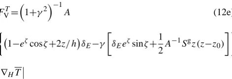
Fig. 12 of C8 (dashed line). In Fig. 2, we compare the pro-files of the fluxesFVT(z)from the present model:
FVT=1+γ2 −1
A (12e)
1−eζcosζ+2z/ h δE−γ
δEeζsinζ+
1 2A
−1Sgz(z−z 0)
∇HT
Fig. 1.−∂zFVT(z)for ICC0 simulation data by Capet et al. (2008)
(dashed curve taken from their Fig. 12) and for the present model (Eq. 12a) (solid curve).
Fig. 2. Profile of the vertical heat fluxFVT(z)for the ICC0 simu-lation data by Capet et al. (2008) (dots) obtained by integrating the dashed curve in Fig. 1, and for the present model (Eq. 12c) (solid curve).
close in the upper half of the mixed layer but differ some-what in the lower half. We think this is due to the similarity of the mean velocity profile (Eq. 8a) with that in the C8 at small depths and by an unavoidable difference in the lower part of the mixed layer due to the different profiles of the ver-tical viscosity used here and in the C8 simulations. While in our analysis we adopted an Ekman profile corresponding to aν(z)= const., C8 adopted a more realistic model forν(z). In spite of that difference, the profiles|u(z)|compare well, as seen in Fig. 3.
7 No-wind case – Buoyancy only
In addition to the realistic case studied by C8, there are data from simulations corresponding to the less realistic case of
u(m s )-1 present model
Capet et al.
z(m)
Fig. 3
Fig. 3. Absolute value of the mean velocity considered in the present analysis which corresponds to the case of a down-front wind and which is given by Eqs. (8a,b), (12b) (solid curve) and the one computed in ICC0 simulation of Capet et al. (2008) (dashed line which is taken from their Fig. 10).
no wind (Fox-Kemper et al., 2008, FFH) which can also be used to test of our model predictions. Following FFH, we as-sume that the mean velocity is in thermal wind balance with the mean buoyancy field and that the mean buoyancy gradient does not vary inside the mixed layer, i.e.,uz=f−1ez×∇Hb
is z independent. Irrespectively of the surface value of u, from Eq. (4b) and the second of Eq. (6b), we derive that:
eu= 1
2f(2z+h)ez×∇Hb, bu= 1
2f(z+h)ez×∇Hb (13a) Takingτ=bin Eq. (6a,b), and using Eq. (13a), the buoyancy flux is given by:
FV(z)=8(γ )
h2 16|f|
1−ξ2|∇Hb|2, (13b)
ξ =1+2zh−1, 8(γ )= 2γ 1+γ2
with:
FV(0)=0, FV(−h)=0, FV(−h/2)=8 ∇Hb
2
>0 (13c) To complete this parameterization ofFV,γmust be obtained
from solving Eq. (7e). Substituting Eq. (13a) into the second of Eq. (7d), we obtain:
V = h
12fez× ∇Hb (14a)
Substituting this result into Eq. (7f), we obtain:
A4=
π2 12(2C)
3/2Ri−1, A
3=0, Ri=
|f|2N2 ∇Hb
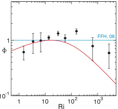
Fig. 4. Richardson number dependence of the two ratios in Eq. (15a, d). The first ratio, represented by full circles with error bars, correspond to updated results from Fox-Kemper’ Comments to our manuscript during the Discussion phase: Ocean. Sci. Dis-cuss. 6, C916–C926, 2009, http://www.ocean-sci-disDis-cuss.net/6/. The results of the present model given by Eq.(15e) withC=6 are shown by the full line. The blue line corresponds to the FFH pa-rameterization,8=1.
The solution of Eq. (7f) is then as follows: γ2=C∗
Ri+
q
Ri2+2Ri/C∗
, C∗= 6 π
2
(2C)3/2(14c) If we employ the valueC=12 that we have determined from the data of Capet et al. (2008), we can compute the function (Eq. 13b):
8(γ )=8(Ri) (14d)
which we exhibit in Fig. 4. We further notice that in spite of the fact noted before that we have only one set of data to determineC, Fig. 5 shows that different C’s have only an overall marginal effect on the buoyancy flux in the interval 1<Ri<100.
Next, we find the limits of applicability of the parameter-izations (Eqs. 13b and 14c,d). To this end, we find the baro-clinic mean kinetic energy averaged over the ML depthKe using the definition (Eqs. 7g, 4b and 13a):
e K= 1
24h
2f−2|∇ Hb|2=
1
12KM (14e)
This result shows that at the surface the mean baroclinic ki-netic energyKeis twelve times smaller than the mean kinetic energyKM=12u2. To compute the SM kinetic energy, we use
the first definition (Eqs. 4b and14c) and derive that: 2KSM=
hN
π γ 2
, γ =γ (Ri) (14f)
Fig. 5. Same as Fig. 4 but with two different values of the parameter
C=3 (dashed), 6 (solid) to show the weak dependence on such a
parameter.
Thus, condition (Eq. 1c) becomes: Ri > π
2
36 3C3/2−1 ∼2×10
−3 (14g)
Next, we compare Eq. (13b) with the FFH data and recall that in their Fig. 14e the authors plot the ratio:
3(data)= FV(data) FV(FFH)
(15a) where:
FV(FFH)=0.06|f|−1h2µ(z)|∇Hb|2, (15b)
µ(z)=(1−ξ2)(1+5ξ2/21) (15c)
is the parameterization suggested by FFH by fitting their sim-ulation data. To compare the model results with the simula-tion data, we construct the ratio:
3(model)=FV(model) FV(FFH)
(15d) Thus,3(FFH)=1, by definition (blue line in Fig. 4). To com-pute Eq. (15d) in our model, we notice that the profile µ(z) in Eq. (15c) has the additional factor(1+5ξ2/21)in com-parison with the profile (Eq. 13b). The difference does not exceed 25% and we neglect it when substituting Eqs. (13b) and (15b,c) into Eq. (15d). As a result, we obtain:
3(present model)=8(Ri) (15e) which we show in Fig. 4 (red line). The present parame-terization yields a good representation of the FFH simula-tion data especially the curvature exhibited by the data. The agreement is somewhat worse at Ri&103which is due to the use of Killworth’s (2005) approximation to neglect τz; in
fact, such an approximation becomes questionable when Ri is large, that is, whenbz=N2 is large. Finally, we discuss
the case with wind. To that end, we take the value ofSg in
the first of Eq. (12b) as determined from C8 simulations and substitute it in Eq. (11b) with the result:
∇Hb≈0.5·10−7s−2 (15f)
Substituting this result in Eq. (15b,c), and using the same mixed layer depthh=40 m as in C8, we obtain:
maxFV(FFH)=2.4·10−9m2s−3 (15g)
If one compares this value with the value from C8 (Fig. 2): maxFV=gαTmaxFVT =2·10
−8m2s−3 (15h)
one concludes that the FFH flux formula with no wind under-estimates the flux by about an order of magnitude, a conclu-sion in agreement with Mahadevan and Tandon (2006) who stressed that “winds play a crucial role in inducing subme-soscale structure” not to mention the multifaceted and im-portant implications on the mixed layer stratification caused by the down-wind, up-wind vs. buoyancy topology described in Sect. 6.
8 Conclusions
Recently, there has been a considerable interest in sub-mesoscales which are oceanic structures of O (1 km) size and life times of the order of days. High resolution numer-ical simulations have been the best source of information to assess the parameterizations of SM fluxes to be used in OGCMs that do not resolve such features. If one consid-ers that the highest resolution of about 1/100in stand-alone OGCMs can represent structures of about 10km size which is 10 times larger than the SM sizes and that OGCMs employed in thousand years runs for climate studies have resolution of about 10 (corresponding to structures 100 times larger than SM), it seems clear that a good deal of important physical processes have thus far gone unrepresented in those OGCMs. The present work presents an analytical parameterization of the SM vertical flux of an arbitrary tracer. The main fea-tures can be described as follows:
(a) no other SM parameterization exists (to the best of our knowledge) that provides an analytical expression for the vertical flux of an arbitrary tracer under arbitrary buoyancy and wind (strength and direction),
(b) the SM parameterization by FFH does not include winds and it is limited to the buoyancy field which cannot be used to describe tracers such as the ones needed in the C-cycle models in OGCMs for climate studies,
(c) the results of the realistic simulations by C8 and MTF with baroclinic instabilities and winds, are well repro-duced by our model,
(d) our parameterization given by Eqs. (4a–c), (7e–f), (12d), is to be used in OGCMs that resolve mesoscales but not sub-mesoscales,
(e) in a different study (Canuto and Dubovikov, 2010), we have derived the parameterization for the tracer verti-cal flux for OGCMs that do not resolve either subme-soscales or mesubme-soscales.
Appendix A
The non-linear termsQH
As discussed in textbooks on Turbulence theories (e.g., Batchelor, 1970; Lesieur, 1990; McComb, 1992), the stochastic Langevin equation has played a major role in tur-bulence modeling studies (Kraichnan, 1971; Leith, 1971; Herring and Kraichnan, 1971; Chasnov, 1991). Though most turbulence models are presented in terms of the energy spec-trum, which is a second-order moment, the starting point is always the Navier-Stokes equations (NSE) presented in the form of a stochastic Langevin equation in k-space:
∂tui(k,t )=fit(k,t )−νd(k)k2ui(k,t )+fiext(k,t ) (A1)
in which the non-linear (NL) term of NSE is represented by the two terms: the turbulent forcingfit(k,t )which is due to the infrared (smallk) part of the NL interactions and ultravi-olet part which is represented by the enhancedk-dependent dynamical viscosity νd(k)=ν+νt(k), where ν is the
kine-matic viscosity whileνt(k)is a turbulent viscosity discussed
in Appendix B. As discussed in the references cited above, the dynamic equation for the energy spectrumE(k) is ob-tained by multiplying Eq. (A1) byu∗i(k0)and integrating over n=k/|k|, the result being:
∂tE(k)=At(k)−2k2νd(k)E(k)+Aext (A2)
where the workAtis given by:
At(k)=k2 Z
dndk0<ui(k0,t )fit(k,t )> (A3)
On the other hand, the general equation forE(k)is given by (Batchelor, 1970, Eq. 6.6.1)
∂tE(k)=T (k)−2νk2E(k)+Aext (A4)
whereT (k)is the non-linear transfer. From Eqs. (A3,A4) it follows that:
T (k)=At(k)−2νt(k)k2E(k) (A5)
Within the closure model developed by Canuto and Dubovikov (1997), the form ofAt(k)is given by:
At(k)= −r(k)
∂E(k) ∂k ,
1 2r(k)=
k Z
0
The key feature of this closure is thatAt(k)is proportional
to the derivative∂kE which vanishes in the vicinity of the
wavenumberk=k0 whereE(k)has its maximum. This
re-duces the two NL terms in Eq. (A1) to the second one only which, in the notation of Eq. (2d,e), implies that:
QuH=k20νd(k0)u0, νd=χd (A7)
Appendix B
Turbulent viscosityνt(k)
Contrary to the kinematic viscosityνwhich does not depend on the size of the eddies, the turbulent viscosityνt(k)which
is due to the NL interactions, depends on the eddy size and its sum toν is called the dynamical viscosity,νd(k)=ν+νt(k).
The search for a suitable expression for νt(k) dates back
many decades and the first explicit expression is the heuris-tic one proposed by Heisenberg as discussed in Batchelor’s book (1970, Sect. 6.6, Eq. 6.6.13),
νt(k)=γ ∞ Z
k
p−3/2E(p)1/2dp γ=O(1) (B1)
whereE(k)is given by Eq. (A2) is the kinetic energy spec-trum whose integral over all wavenumbers yields the eddy kinetic energyKE. As discussed by Batchelor, Eq. (B1) was
successfully used to derive the Kolmogorov spectrum. A non heuristic derivation ofνt(k)has however been lacking
un-til recently with the advent of methods to treat the Navier-Stokes equation borrowed to a large extent from quantum field theory. A full presentation was made by the present authors in 1997 with the final result:
νt(k)=
ν2+ 1 2
∞ Z
k
p−2E(p)dp
1/2
(B2)
Equation (B2) has several interesting features worth dis-cussing. First, it says that an eddy of arbitrary size (∼k−1) feels the effects of all the eddies smaller than itself, as the in-tegral begins at k and accounts for all the wavenumbers from k to infinity. Equation (B2) naturally reduces to the kine-matic viscosityνwhen the size of the eddy is very small and ktends to infinity. Due to the presence of the kinematic vis-cosity, Eq. (B2) is valid for arbitrary Reynolds number since it can be rewritten as:
νt(k)=ν h
1+Re(k)2 i1/2
, Re(`)∼`K
1/2
ν (B3)
If one employs the Kolmogorov spectrum
E(p)=Koε2/3k−5/3, one obtains in the large Re regime:
Re1: νt(k)= ν2+
3Ko 16
ε2/3 k8/3
!1/2
≈ε1/3`4/3 (B4)
which is the well-known Richardson 4/3 law diffusivity ∼`4/3. Finally, relation (Eq. B2) shows that there is no such a thing as a unique turbulent viscosity since each eddy feels its own turbulent viscosity. In Eqs. (2e) and (3a) we are inter-ested in the functionνt(k)≈νd(k)in the vicinity of the
max-imum of the energy spectrumk=k0. Assuming that most of
the energy is contained in that region, from Eq. (B2) we de-rive thatνd∼k0−1KE1/2. Thus, from Eq.!(A7) it follows that: QuH =k1/2
0KE u 0
(B5) which is the closure form in Eq. (3a). The closure for the tracer field is analogous.
Appendix C
Derivation of Eq. (4)
C1 Sub-mesoscale tracer fieldτ0
Substituting Eq. (3a) into the tracer Eq. (2e), we obtain the following expression for the submesoscale tracer field: τ0= u
0· ∇ Hτ
χ+i(k·u−ω) (C1)
where|k|=k0=rS−1. As in the case of mesoscales discussed
in CD5, the frequencyω is obtained by solving the eigen-value problem mentioned below Eq. (3a) with the following result (dispersion relation):
ω(k)=k·ud (C2)
This relation can be interpreted as the Doppler transforma-tion for the frequency provided that in the system of coor-dinates moving with velocityud, the submesoscale flow is
stationary, in which caseω=0. Stated differently, relation (Eq. C2) implies thatud is the eddy drift velocity whose
ex-pression in terms of mean fields is analogous to that for the case of mesoscales given in Eq. (4f) of CD6:
ud=<u>+1 2`
2e
z×(β−f <∂zs>) (C3)
wheres=−∇Hb/N2 is the slope of isopycnal surfaces and
β=∇f. The bracket averaging is defined as follows:
<•> ≡
0 Z
−h
(•)KSM1/2(z)dz/
0 Z
−h
KSM1/2(z)dz (C4)
Due to the smallness of the scale ` characterizing subme-soscales, the second term in Eq. (C3) is negligible and thus in good approximation we have that:
which changes Eq. (C1) to the form: τ0= − u
0· ∇ Hτ
χ+ik· eu
, eu=u−<u>, χ=`−1KS1/2 (C6) Relation (Eq. C2) implies that the dependence of the subme-soscale fields onωis of the form:
A0(ω,k)=A0(k)δ(ω−k·ud) (C7)
and therefore in the(t,k)-space the fieldsA0depend on time as follows:
A0(t,k)=A0(k)exp(−ik·udt ) (C8)
Due to relations (Eqs. C7,C8), after substituting Eq. (3a) in Eq. (2e), the latter may be solved in both (ω, k) and (t,k) representations.
C2 Sub-mesoscale velocity fieldw0
It is convenient to begin by splitting the mesoscale velocity fieldu0 into a rotational (divergence free, solenoidal) and a divergent (curl free, potential) components:
u0(k)=uR(k)+uD(k); uR(k)=n×ezuR(k), (C9) uD(k)=nuD, n=k/ k
and thus the third equation in Eq. (2e) becomes:
∂zw0= −ik·u0= −ikuD (C10)
To determineuR,D, we substitute the second relation (Eq. 3a)
in the second equation in Eq. (2e) and derive the following expressions:
uD=f−1(χ+ik·eu)uR (C11)
uR= −
ikρ−1p0 1+f−2(χ+ik·
eu)
2, eu=u−<u> (C12) These relations, as well as Eq. (C6), are valid in both (ω,k) and (t,k) representations. Below, we will use them in the (t,k) representation together with Eq. (C8). Due to the third relation of Eq. (3a), the further use of Eqs. (C11) and (C12) is considerably simplified under the condition
KSM/Ke1 (C13)
which allows us to neglect the second terms in the brackets in Eqs. (C11) and (C12). Condition (Eq. C13) coincides with Eq. (1c).
C3 Spectrum of the vertical SM flux
In the dynamical Eq. (1a) one needs∂zFV which we shall
write as follows: ∂zFV=w0zτ0+w0τ0
z≈w 0
zτ0 (C14)
where in the last expression we have neglected the termw0τ0 z
in accordance with the adopted approximation τ0 and be-cause it is of a higher order in z. Substituting Eq. (C11) into Eq. (C10), we obtain the expression for∂zw0 which allows
us to compute∂zFVusing Eq. (C14).
The strategy of computing submesoscale fluxes, which are bilinear correlation functions, consists in computing these functions in(t,k)-space which, in the approximation of ho-mogeneous and stationary mean flow, have the form: A0(t,k0)B0∗(t,k)=A0B0∗(k)δ(k−k0
) (C15)
which, because of relation (Eq. C8), does not depend ont. The function ReA0B0∗(k)is usually referred to as the density ofA0B0in k-space. The spectrum of the correlation function A0B0is:
A0B0(k)= Z
ReA0B0∗(k)δ(k− |k|)d2k (C16)
i.e., the spectrum of A0B0 is obtained by averaging ReA0B0∗(k)over the directions of k and multiplying the re-sult byπ k. Finally, the correlation functionA0B0 in physi-cal space is obtained by integrating over the spectrum. Fol-lowing this procedure, from the first of Eq. (C6) and using Eqs. (C9,C10), we derive the relation:
Re w0
zτ0∗(k)= (C17)
−I mnkχ2(χ +ik· eu)
h
uDu∗R(k)n×ez+|uD|2(k)n io
· ∇Hτ
Next, from Eqs. (C11,C12) we derive the following relations: Re uDu∗R(k)=χf
−1|u
R|2(k), (C18)
I m uDu∗R(k)=f −1k·
eu|uR| 2(k)
|uD|2(k)=χ2f−2|uR|2(k), |u0|2(k) (C19)
= |uD|2(k)+ |uR|2(k)=(1+χ2f−2)|uR|2(k)
Substituting Eq. (C18) into Eq. (C17) and averaging over the directions of k, we obtain the spectrum ofw0
zτ0(k). Under
conditions (Eq. C13), we get: w0
zτ0(k) (C20)
= −k20bχ−2hχf−1|uR|2(k)eu×e+ |uD| 2
where:
π k|uR|2(k)=2
1+χ2f−2 −1
E(k), π k|uD|2(k) (C21)
=21+χ−2f2 −1
E(k), E(k)=1 2π k|u
0|2(k)
whereE(k)is the spectrum of the total (rotational + diver-gent) eddy kinetic energy. Due to relation (Eq. C14), the left hand side of Eq. (C20) multiplied byπ kis the spectrum of the z-derivative of the vertical flux∂zFV(k). Thus,
mul-tiplying Eq. (C20) byπ k, using Eq. (C21), we obtain the following expression for the spectrum of ∂zFV(k)near the
maximum of the energy spectrum:
∂zFVτ(k)=8(k)· ∇Hτ (C22)
where:
8(k)= −2E(k)k02χ−2 (C23)
h
χf−1(1+χ2f−2)−1eu×ez+(1+χ−2f2)−1eu i
Assuming that the spectra FV(k) and E(k) have similar
shapes, integration of Eqs. (C22,C23) overkreduces to the substitution ofE(k)andFV(k)with the eddy kinetic energy
KSMandFVin physical space. Thus, we get Eq. (4a,b).
Acknowledgements. The authors thank Reviewer #1 for requesting clarifications on Sect. 7 and Reviewer #2 for very valuable suggestions that helped us improve the overall presentation.
Edited by: E. J. M. Delhez
References
Batchelor, G. K.: The theory of homogeneous turbulence, Cam-bridge Univ. Press, 195 pp., 1970.
Boccaletti, G., Ferrari, R., and Fox-Kemper, B.: Mixed layer insta-bilities and restratification, J. Phys. Oceanogr., 37, 2228–2250, 2007.
Canuto, V. M. and Dubovikov, M. S.: A new approach to turbu-lence, Int. J. Mod. Phys., 12(18), 3121–3152, 1997.
Canuto, V. M., Dubovikov, M. S., and Yu, G.: A dynamical model for turbulence, IX. Reynolds stress spectra for shear-driven flows, Phys. Fluids, 11(3), 676–691, 1999.
Canuto, V. M. and Dubovikov, M. S.: Modeling mesoscale eddies, cited as CD5, Ocean Model., 8, 1-30, 2005.
Canuto, V. M. and Dubovikov, M. S.: Dynamical model of
mesoscales in z- coordinates, cited as CD6, Ocean Model., 11, 123–166, 2006.
Canuto, V. M. and Dubovikov, M. S.: Derivation and assessment of a mixed layer sub-mesoscale model, cited as CD9, Ocean Sci. Discuss., 6, 2157–2192, doi:10.5194/osd-6-2157-2009, 2009. Canuto, V. M., Dubovikov, M. S., Luneva, M., Clayson, C. A., and
Leboissetier, A.: Mixed layer mesoscales: a parameterization for OGCMs, Ocean Sci. Discuss., 7, 873–917, doi:10.5194/osd-7-873-2010, 2010.
Canuto, V. M. and Dubovikov, M. S.: Mixed layer sub-mesoscale parameterization - Part 2: Results for coarse resolution OGCMs, Ocean Sci. Discuss., 7, 1289–1302, doi:10.5194/osd-7-1289-2010, 2010.
Capet, X., McWilliams, J. C., Molemaker, M. J., and Shchepetkin, A. F.: Mesoscale to submesoscale transition in the California cur-rent system, Part I: flow structure, eddy flux, and observational tests, J. Phys. Oceanogr., 38, 29–43, 2008.
Chasnov, J. R.: Simulation of Kolmogorov inertial subrange using an improved subgrid model, Phys. Fluids, A3, 188–193, 1971. de Boyer Montegut, C., Madec, G., Fisher, A. S., Lazar, A., and
Iu-dicone, D.: Mixed layer depth over global ocean: an examination of profile data and a profile-based climatology, J. Geophys. Res., 109, C12003, doi:10.1029/2004JC002378, 2004.
Fox-Kemper, B., Ferrari, R., and Hallberg, R.: Parameterization of mixed layer eddies I: theory and diagnostics, J. Phys. Oceanogr., 38, 1145–1165, 2008.
Fox-Kemper, B. and Ferrari, R.: Parameterization of mixed layer eddies II: prognostics and impact, J. Phys. Oceanogr., 38, 1166– 1179, 2008.
Herring, J. R. and Kraichnan, R. H.: Comparison of some approxi-mations for isotropic turbulence, in: Statistical Models and Tur-bulence, edited by: Rosenblatt, M. and Van Atta, C., Springer-Verlag, New York, 147–194, 1971.
Hosegood, P. J., Gregg, M. C., and Alford, M. H.: Restratification of the Surface Mixed Layer with Submesoscale Lateral Density Gradients: Diagnosing the Importance of the Horizontal Dimen-sion, J. Phys. Oceanogr., 38, 2438–2460, 2008.
Killworth, P. D.: On parameterization of eddy transport, J. Mar. Res., 55, 1171–1197, 1997.
Killworth, P. D.: Parameterization of eddy effect on mixed
layer tracer transport: a linearized eddy perspective, J.Phys. Oceanogr., 35, 1717–1725, 2005.
Klein, P., Hua, B. L., Lapeyre, G., Capet, X., Le Gentil, S., and Sasaki, H.: Upper ocean turbulence from high resolution 3D sim-ulation, J.Phys. Oceanogr., 38, 1748–1763, 2008.
Kraichnan, R. H.: An almost Markovian Galilean invariant turbu-lence model, J. Fluid Mech., 47, 513–524, 1971.
Kraichnan, R. H.: Statistical dynamics of two-dimensional flow, J. Fluid Mech., 67, 155–171, 1975.
Lapeyere, G., Klein, P., and Hua, B.C.: Oceanic re-stratification forced surface frontogenesis, J. Phys. Oceanogr., 36, 1577–1590, 2006.
Leith, C. E.: Atmospheric predictability and two-dimensional tur-bulence, J. Atmos. Sci., 28, 145–161, 1971.
Lesieur, M.: Turbulence in Fluids, section 3.3, Kluwer, Dordrecht, 212 pp., 1990.
Levy, M., Klein, P., and Treguier, A. M.: Impacts of sub-mesoscale physics on production and subduction of phytoplankton in an oligotrophic regime, J. Mar. Res., 59, 535–565, 2001.
Levy, M., Klein, P., Treguier, A. M., Iovino, D., Madec, G., Mas-son, S., and Takahashi, K.: Modification of gyre circulation by submesoscale physics, Ocean Model., 34, 1–16, 2010.
Mahadevan, A.: Modeling vertical motion at ocean fronts: Are non-hydrostatic effects relevant to sub-mesoscales?, Ocean Model, 14, 222–240, 2006.
Mahadevan, A., Tandon, A., and Ferrari, R.: Rapid changes in mixed layer stratification driven by sub-mesoscales instabili-ties and wind, cited as MFT, J. Geophys. Res., 115, C03017, doi:10.1029/2008JC005203, 2010.
Maltrud, M. E. and McClean, J.L.: An eddy resolving 1/100ocean simulation, Ocean Model., 8, 31–54, 2005.
McComb, W. D.: The Physics of Fluid Turbulence, Oxford Science Publications, Oxford, UK, 572 pp., 1992.
Nurser, A. J. G. and Zhang, J. W.: Eddy-induced Mixed Layer Shal-lowing and Mixed Layer-Thermocline Exchange, J. Geophys. Res., 105(C9), 21851–21868, 2000.
Provenzale, A.: Transport by coherent barotropic vortices, Ann. Rev. Fluid Mech., 31, 55–93, 1999.
Sasaki, H., Nonaka, M., Masumoto, Y., Sasai, Y., Uehara, H., and Sakuma, H.: An Eddy Resolving Hindcast Simulation of the Quasiglobal Ocean from 1950 to 2003on the Earth Simulator, in: High Resolution Numerical Modeling of the Atmosphere and Ocean, edited by: Ohfuchi, W. and Hamilton, K., Springer, 157– 186, 2008.
Spall, M. A.: Frontogenesis, subduction, and cross-front exchange at upper ocean fronts, J. Geophys. Res., 100, 2543–2557, 1995. Thomas, L. N.: Destruction of potential vorticity by winds, J. Phys.
Oceanogr., 35, 2457–2466, 2005.
Thomas, L. N. and Lee, C. M.: Intensification of ocean fronts by down-front winds, J. Phys. Oceanogr., 35, 1086–1102, 2005. Thomas, L. N., Tandon, A., and Mahadevan, A.: Submesoscale
processes and dynamics, in: Eddy Resolving Ocean Modeling, edited by: Hecht, M. and Hasumi, H., AGU Monograph, Ameri-can Geophysical Union, Washington, DC, 17–38, 2008. Treguier, A. M., Theetten, S., Chassignet, E., Penduff, T., Smith, R.,