Applications
Mohamed Aboraya
Department of Applied Statistics and Insurance, Damietta University, Egypt. e-mail: [email protected]
Abstract
In this article, we introduce a new lifetime model which exhibits the increasing, the decreasing and the bathtub hazard rates. The considerable justification for the practicality of the new lifetime model is depended on the wider use of the exponentiated Weibull and Weibull lifetime models. The new lifetime model can be viewed as a mixture of the exponentiated Weibull distribution. It can also be viewed as an appropriate model for fitting the right skewed, the symmetric, the left skewed and the unimodal data. We prove empirically the importance and flexibility of the new model in modeling two types of lifetime data.
Keywords: Hazard rates; Weibull lifetime model; Exponentiated weibull.
1. Introduction
A random variable (r.v.) Z is said to have the exponentiated Weibull (E-W) distribution if its probability density function (PDF) given by
( ) 1 1
( ; , ) 1 ,
E W z z
g z z
−
− = − − − −
e e (1)
and cumulative distribution function (CDF)
( )
( ; , ) 1 ,
E W z
G z
− = − −
e
(2) respectively, for z0 , 0 and 0 .The PDF and CDF of the Odd Lindley (OL-G) family of distribution (Silva et al. (2017)) are given by
(
)
1 ( ) ( ); / ;( ) ( )
32
( ; , ) 1 aG x G x ; ; ,
f x a =a +a − e− g x G x −
(3) And
(
)
1 ( ) ( ); / ;( ) ( )
1( ; , ) 1 1 aG x G x ; ; ,
F x a = − +a − e− a G x+ G x −
(4) respectively. To this end, by using equations (1), (2) and (3) to obtain the three-parameter OLEW density (5). A r.v. X is said to have the OLEW distribution if its PDF and CDF are given by
(
)
12 1
3 1
1 / 1 1 ( ) 1
1 1 1
, 0
x x
x
x x
a
f x a a x
x
− −
− − −
− −
− −
− − − −
= +
− − −
e e
e
e e
e (5)
(
)
1
1
1 / 1 1
( ) 1 1 1
1 1 1
, 0
x x
x
x
a F x
a a
x
− −
− −
− −
− − − −
= − − −
+ + − −
e e
e
e
e
(6) respectively. The PDF of X in (5) can be easily expressed as
( )
(
(
)
)
, , 0
( ) i k E W ; 1 , , i k
f x g x i k
−
=
=
+ +(7) where
( )
(
) (
)
1(
) (
)
2
, 1 1 1 ! 3 / 3 ,
k k
i k a i k a i i k k
= − + + + + − + + +
and g(E W− )
(
x i;(
+ +k 1)
,)
is PDF of E-W model with positive parameters(
i+ +k 1)
and . The CDF of X can be given by integrating (7) as( )
(
(
)
)
, , 0
( ) i k E W ; 1 , ,
i k
F x x i k
−
=
=
+ +(8) where
( )
(
(
)
)
( )(
(
)
)
; 1 , ; 1 ,
E W E W
x i k G x i k
− −
+ + = + +
is PDF of E-W model with positive parameters
(
i+ +k 1)
and . For more details about the OL-G family see Silva et al. (2017). For more information about the E-W model see Mudholkar and Srivastava (1993) and Nadarajah and Kotz (2006).2. Graphical presentation and justification
Figure 1: Plots of the OLEW PDF.
Figure 2: Plots of the OLEW HRF
well as bathtub hazard rates (see Figure 2). The new model can be viewed as a mixture of the E-W density. It can also be considered as a convenient model for fitting the symmetric, the left skewed, the right skewed, and the unimodal data (see applications 1, 2, 3, and 4). The new lifetime model is a superior on the Marshall Olkin extended-Weibull, the Poisson Topp Leone-extended-Weibull, the Burr X Exponentiated-extended-Weibull, the Kumaraswamy-Weibull, the Gamma-Weibull, the Transmuted modified-Weibull, the Weibull-Fréchet, the Beta-Weibull, the Mcdonald-Weibull, the transmuted exponentiated generalized-Weibull, the Kumaraswamy transmuted-Weibull, and the Modified beta-Weibull models so the new model is a good substitutional to these models in modeling the aircraft windshield data. The new lifetime model is much better than the Mcdonald-Weibull, the transmuted linear exponential, the Mcdonald-Weibull, the transmuted modified-Weibull, the Modified beta-modified-Weibull, the transmuted additive-modified-Weibull, the exponentiated transmuted generalized Rayleigh models in modeling cancer patient data. In modeling the survival times of Guinea pig's data, we deduced that the proposed model is much better than the Odd Weibull-Weibull, the Weibull Logarithmic-Weibull and the gamma exponentiated-exponential models. Finally, the new model is a preferable model than the exponentiated-Weibull, the transmuted-Weibull, the Odd Log Logistic-Weibull models, and a good alternate to these models in modeling Glass fibers data.
3. Shapes
The critical points of the OLEW density function are the roots of the equation 1 1 1 1 1 1 1 1 2 1 0 1 1 3 1 1 1 . 1 1 x x d dx x x x x x x x x x x x x a − − − − − − − − − − − − − − − − − − − = − − + − − − + − − e e e e e e e e e e
We can examine the last two Equations to determine the local maximums and minimums and inflexion points via most computer algebra systems.
4. Statistical Properties
Quantile functions
Let X be an arbitrary r.v. with CDF F x a( ; , , ) . For any U
( )
0.1 , the u th quantile function (QF) Q U( ) of the r.v. X is the solution of u=F Q U(
( ))
for all Q U( )0,from Equ. (6), we get
(
)(
)
1(
)
(
)
1 (((( ))))1 1 1 ( ) / 1 ( ) ,
aG Q U G Q U
a
u− +a e+ = − + − a G Q U −G Q U e−−
where
(
)
(
)
1 a G Q U( ) / 1 G Q U( )
− + − −
is the Lambert W function of the real argument
(
1+a u)(
−1 exp 1)
(
+a)
and the Lambert W function is defined as( )
( ). W x
W x e =x
From Silva et al. (2017), we can write the following equation for qf of the OLEW model
( )
(
(
)(
)
)
1 1 1
log 1 1 a ,
Q u a W u a
+
= − − − − +
e
where W
( )
is Lambert function.Moments
The rth ordinary moment of X is given by r 0 x f x dxr
( )
E X( r). = =
Using (7), we
get
( )
( ) / 1
(
)
1 ,,
, , 0 0
/ , ,
r i k r r i k j
i j k m
c r m r
+ + −
= =
=
− −(9) where
( , )
( ) (
)
( )/ 11 1 r ,
r
c
− + −
= − +
(
)
1(
) (
)(
)
0
1 1 2 ...1, R
v m
v v m v v v v
−
+
=
+ =
− = − − and
( )
10
t
x e dx
− −
=
is the complete gamma function. The rth incomplete moment of X , say r
( )
t , is given by r( )
t = 0tx f x dxr( )
. Using Equ. (7), we obtain( )
(
1)
(( 1) , ), , , 0
1 , i k r , ,
r i k j
i j k
t r t c r
− − + +
=
= +
−(
)
10 ,
x
x
x− e dx− = x
is the incomplete gamma function.
The skewness of the new distribution can range in the interval (3.0, 13.29), whereas the kurtosis of the new distribution varies only in the interval (16.24, 342.27) also the mean of X increases as a decreases, the skewness is always positive (see Table 1 below). Kurtosis and skewness decreases as a decreases.
Order statistics
Let X1,K,Xn be a random sample (RS) from the OLEW model of distributions and let 1 : 1, , n:n
X K X be the corresponding order statistics, so the PDF of the ith order statistic, say Xi:n , can be expressed as
( )
1 1:
0
( 1) ( , 1) ( ) ( ) .
n i
j j i
i n
j
n i
f x B i n i f x F x
j −
− + −
=
−
= − − +
where B( , ) is the beta function. Substituting (5) and (6) in Equ. of fi:n
( )
x , we obtain( )
( )(
(
)
)
: , ,
, 0 0
; 1 , ,
k n i
E W
i n i m p
m p j
f x g x j m p
+ − − = = =
+ + + where( )
(
)
( )
(
)
1 1 1 2 , , 0 11 1 B( , 1)
1 1
! 1 .
i
k m j m j
i m p k
a a i n i
j m p k n i
m j m p
j m j k
− + + + − + − = − = − + − + + + + − − + + + +
Then, the zth moment of Xi:n is given by
(
)
(( 1) , ) / 1(
)
: , ,
, , 0 0 0
/ , .
z k n i
j m p z z
i n i m p h
m p h j w
E X c z w z
− + − + + + = = = =
− −Moment of Residual and Reversed Residual Life (MRL & MRRL)
The nth MRL is given by
1,2,
( ) [( ) |n n ], 0.
n X t
z t =E X −t = K t So, the nth MRL of X can be given as
11 ( ) ( )n ( ) n( ), t
F t − x t dF x z t
−
− =Subsequently, we can write
( )
(
(
)
)
(
)
(( ) )1
, , 0 0
1 1 ,
1
, , , , , 0 0
( ) 1 ( ) ; 1 , ,
1 , 1 ( ) ,
n
n r r
n i k t
i k r
n
i k n i j k r i j k r
n
z t F t t x g x i k dx
r
n t F t n
− − = = − + + − − = = = − − + + = + − −
where ( )( 1 , )
(
) ( )
(
)
( )/, , , , 1 1 1 .
i n r n i k n n r
i j k r i k
i k n
t i k j
j r + + = − + + − + − + − + +
The nth MRRL is given by
1, 2,
( ) ( ) |n n , 0 ,
n X t
Z t =E t−X = K t uniquely determines F x( ) . We have
1 0
( ) t( )n ( ) n( ).
F t −
t−x dF x =Z tThen, the nth moment of the reversed residual life of X becomes
( )
(
(
)
)
(
)
(( ) )1
, 0 , 0 0
1 ,
1 1
, , , , , 0 0
( ) ( ) 1 ; 1 , ,
1 , ( ) ,
n t
r n r r
n i k
i k r
n
i k n i j k r i j k r
n
Z t F t t x g x i k dx
r
n t F t n
− − = = + + − − − = = = − + + = + −
where ( )( 1 , )
(
) ( ) (
)
( )/, , , , 1 1 1 .
i r n
i k n n r i j k r i k
i k n
t i k j
5. Maximum likelihood method
If x1,K,xn be a RS of the new distribution with parameter vector =( , , , )a T . The log-likelihood function for , say L =L( ) , is given by
(
)
(
)
(
)
(
)
1 1 1
1 1
( ) 2 log 2 log 1 log log
1 log 3 log 1
1 log
n n n
i i i
i i i
n n
i i
i i
L L n n a n n
x x s
s a z
= = = = = = = − + + + + − − − − + − −
where(
)
11 x and 1 ,
i i i i
s z s s
−
−
= − = −
e
Equ. of L( ) can be maximized either via the different programs like R (optim function), SAS (PROC NLMIXED) or via solving the nonlinear likelihood equations obtained by differentiating Equ. (13). The score vector elements,
( )
L(
L, L, L)
T a
= =
U , are given as
1 1 n i i L n z
a a =
= − −
+
1 1
log
3 log ,
1
n n
i i
i
i i i
s s L n s s = = = + +
−
and(
)
11 1 1 1 1
log log 3 1 ,
1
n n n n n
i i i
i i i i
i i i i i i i
s m m
L n
x x x a w
s s − = = = = = = + − + + − −
−
where(
)
1 2log and ,
1
x i i
i i i i
i
m s
m x x w
s − − = = − e
we can obtain the estimates of the unknown parameters via setting the score vector to zero,
^ ( )=
U 0 , then solving these equations simultaneously gives the MLEs ^ ^
,
a and ^
.
6. Data modeling
In this section, we provide four applications of the OLEW distribution to demonstrate empirically its significance, we consider the Cramér-von-Mises ( *
W ) and the Anderson-Darling (A*) statistics. These statistics can be written as
(
)
(
)
2(
)
*1
1/12 n i 2 1 / 2 1 1/ 2
j
n = z j n n W
+ − − + =
(
)
(
)
* 12 1
9 3 1
1 2 1 log 1
4 4
n
i n j j
n j z z A
n n n = − +
+ + + − − =
respectively, where zi =F y
( )
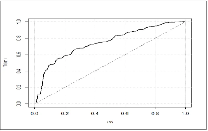
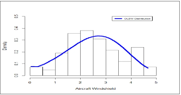
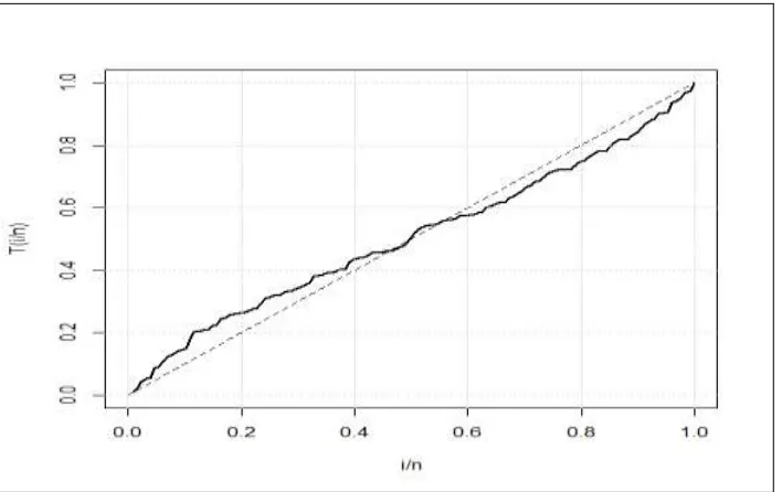
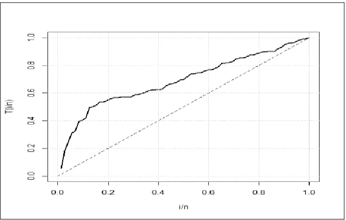
j and the yj 's values are the ordered observations. The required calculations are carried out via the R software. The MLEs and the corresponding standard errors (SE) (in parentheses) of the model parameters are given in Tables 2, 3, 4, and 5. The numerical values of the statistics *W and A* are listed in the same Tables. The histograms of the four data sets are displayed in Figures 4, 6, 8, and 10. the total time test (TTT) (see Aarset (1987)) are displayed in Figures 3, 5, 7, and 9
Application 1: Failure times of 84 aircraft windshield
The data consist of 84 observations. The data are: 0.0400, 1.8660, 2.3850, 3.4430, 0.3010, 1.8760, 2.481, 3.4670, 0.3090, 1.899, 2.6100, 3.478, 0.5570, 1.911, 2.6250, 4.570, 1.6520, 2.3000, 3.344, 4.6020, 1.757, 3.5780, 0.9430, 1.912, 2.6320, 3.595, 1.0700, 1.9140, 2.6460, 3.699, 1.1240, 1.9810, 2.661, 3.7790, 1.2480, 2.010, 2.2240, 3.1170, 4.485, 1.6520, 2.229, 3.1660, 2.688, 3.9240, 1.2810, 2.0380, 2.823, 4.0350, 1.281, 2.0850, 2.890, 4.1210, 1.303, 2.0890, 2.902, 4.1670, 1.432, 4.3760, 1.615, 2.2230, 3.114, 4.4490, 1.619, 2.0970, 2.934, 4.240, 1.4800, 2.135, 2.9620, 4.255, 1.5050, 2.154, 2.9640, 4.278, 1.50600, 2.190, 3.0000, 4.3050, 1.5680, 2.1940, 3.1030, 2.3240, 3.3760, 4.6630. Figure 3 gives the TTT plot for the data set I. From Figure 3, we note that the HRF of data set I is increasing.
Figure 3: TTT plots for data set I.
( ) 1 2 1 3
1
2 2
( ) 2 1 1 1
1 1
exp 1 exp
1 1 1 1
BrX E W x x x
x x
x x
f x x
− − − − − − − − − − − − = − − − − − − − − − − − −
e e e
e e
e e
the Beta-Weibull (B-W) (Lee et al., 2007)
( )
( )
1( )
1
( )
1 ( ), 1 ;
a
TM W x b x
f x B a b x
−
− = − − −e− e−
the Poisson Topp Leone-Weibull (PTL-W)
( ) 1 1 2 2 1 1 2
( ) 2 1 1 ;
b x
b b
PTL W b b x x
f x ba x e
− − − − − − = − − − − − − e
e e e
the Transmuted modified-Weibull (TM-W) (Khan and King, 2013)
( )
( )
(
1)
1 2 , 1;
TM W x x x x
f − x = + x− − + e− − e− −
Marshall Olkin extended-Weibull (MOE-W) (Ghitany et al., 2005)
( )
(
)
( ) 2 1 ( )( ) 1 1 ;
MOE W x x
f x x
−
− = − − − − −
e e
th transmuted exponentiated generalized Weibull (TExG-W) (Yousof et al., 2015)
( )
( )
1
1 ( ) ( )
( )
1
1 2 1 , 1.
b
TExG W a x a x
b a x
f x ab x
− − − − − − = − + − − e e e
the Gamma-Weibull (Ga-W) (Provost et al., 2011)
( ) / 1 1
(
)
1( ) 1 / ;
Ga W x
f − x = +− + x + −e−
the Weibull-Fréchet (W-Fr) (Afify et al., 2016c)
( ) ( )
( )
( ) ( )( )
1 1
( ) 1 exp ,
1 b x x x x b b b b b
f x ab x a
− + − − − + − − = − − − e e e e
the Kumaraswamy-Weibull (Kw-W) (Cordeiro et al., 2010)
( )
( )
1 1 ( ) 1 ( ) 1 1 ( ) 1;b
a a
W Fr x x x
f x ab x
− −
− = − − − − − − −
e e e
( )
(
)
1 ( ) ( )
1 2
( ) ( )
1
( ) ( )
( ) 1 2 1
1 1 1 1
1 1 1 ;
KwT W x x
b a
x x
a
x x
f x a b x
− − − − − − − − − − = + − − − + − − − − + − − e e e e e e
Modified beta-Weibull (MB-W) (Khan, 2015)
( )
( )
( )
( )
( )(
)
( )
1
1 1
, 1
1 1 1 ;
x x
x
a b
MB W a
a b b
f x B a b x
− − − − − − − − − − = − − − − e e e
the Mcdonald-Weibull (Mc-W) (Cordeiro et al., 2014),
( )
(
)
1 ( ) 1 1
1 ( )
1 ( )
( ) / ,
1 1 ;
a x
Mc W x
b c x
f x c B a c b x
− − −− − − − − − = − − e e e
distributions, whose PDFs (for x0 ). The parameters of the above densities are all positive real numbers except for the TM-W and TExG-W distributions. Some other extensions of the W distribution can also be used in this comparison, but are not limited to Yousof et al. (2015), Afify et al. (2016b, c), Yousof et al. (2016a, b), Cordeiro et al. (2017a, b), Yousof et al. (2017a, b, c, d, e), Korkmaz et al. (2018am b), Brito et al. (2017), Hamedani et al. (2017) and Hamedani et al. (2018a, b). The figures in Table 1 proves that the OLEW distribution yields the lowest values of *
W and A* , hence he OLEW distribution provides the best fit to the two data sets
Based on the figures in Table1 we conclude that thehe OLEW distribution provides adequate fits as compared to other Weibull models with small values for W⚫andA⚫ . The proposed lifetime model is better than the MOE-W, Ga-W, BrXE-W, PTL-W, Kw-W, KwT-Kw-W, MB-Kw-W, Mc-Kw-W, W-Fr, B-Kw-W, TM-Kw-W, and TExG-W models, and a good ersatz to these models.
Application 2: Cancer patient data
Figure 5: TTT plots for data set II.
We compare the fits of the OLEW distribution with other competitive models, namely: the McW, transmuted linear exponential (TL-E) (Tian et al., 2014)
( )
(
)
( 2)
( 2)
2 2
( ) 1 x x 1 2 x x , 1;
TL E
f x x
− + − +
− = + − − +
e e
The TMW, MBW, exponentiated transmuted generalized Rayleigh (ETGR) (Afify et al., 2015)
( )
( )
(
( ))
( )( )
(
)
2 2 2
2
1 1
( ) 2
1
1 1 1
2 , 1
1 2 1
x x x
ETG R
x
f x x
− −
− − −
−
− −
+ − − −
=
+ − −
e e e
e
and the W (Weibull, 1951)
( )W
( )
1 ( )xf x x
− −= e
transmuted additive Weibull distribution (TA-W) (Elbatal and Aryal, 2013)
( )
(
1 1)
(
)
(
)
( ) x x 1 2 x x ;
TA W
f x x x
− +
− +− = − + − e − + e
Figure 6: Estimated PDF for data set II.
Based on the figures in Table 2 we conclude that the proposed lifetime model is much better than the Mc-W, TL-E, W, TM-W, MB-W, TA-W, ETG-R models with small values for ?
Application 3: Survival times of Guinea pigs
The second real data set corresponds to the survival times (in days) of 72 guinea pigs infected with virulent tubercle bacilli reported by Bjerkedal (1960). The data are: 10, 33, 327, 342, 347, 361, 72,74, 77, 92, 93, 215, 216, 222, 113, 115, 116, 120, 121, 197, 230,231, 240, 245, 108, 108, 108, 109, 112, 122, 72, 176, 183, 122, 124, 130, 134, 136, 139, 144, 146, 153, 159, 160, 163, 163, 168, 171, 195, 96, 100, 100, 102, 105, 107, 107, 202, 213, 196, 251, 253, 254, 255, 278, 293, 402, 432, 458, 44, 56, 59, 555. Figure 7 gives the TTT plot for the data set III. From Figure 7, we note that the HRF of data set III is increasing.
Figure 7: TTT plots for data set III.
We shall compare the fits of the OLEW distribution with those of other competitive models, namely: Odd Weibull-Weibull (OW-W) (Bourguignon et al., 2014)
( )
( )
( ) 1 exp exp 1 ;
OW W
f − x = − − x −
the gamma exponentiated-exponential (GaE-E) (Ristic and Balakrishnan 2012)
( )
( )
1 1
( ) 1 log 1 ;
x
GaE E x x
f x
− − −
− = − − + − − −
e
e e
Figure 8: Estimated PDF for data set III.
Based on the figures in Table 3 we conclude that the proposed model is much better than the OW-W, WLog-W, GaE-E models, and a good alternative to these models in modeling survival times of Guinea pigs.
Application 4: Glass fibres data
Figure 9: TTT plots for data set IV.
For this data set, we shall compare the fits of the OLEW distribution with some competitive models like E-W, T-W:
( ) 1
( )
( )
( ) exp 1 2 1 exp , 1,
T W
f x x x a a x a
− = − − + − − −
and OLL W:
( )
( )
( )( )
( )1 1
2
( ) 1
1 .
OLLW x x
x x
f x x
−
− −
−
−
− −
= −
− +
e e
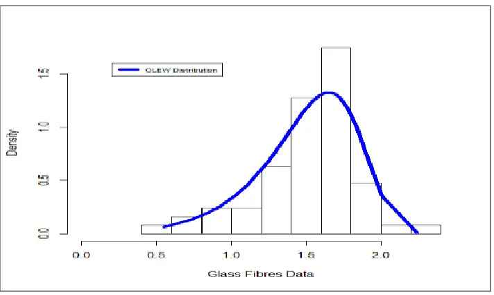
Figure 10: Estimated PDF for data set IV.
Based on the figures in Table 4 we conclude that the proposed model is much better than the E-W, T-W, OLL-W models, and a good alternative to these models in modeling glass fibres data.
Concluding remarks
In this article, we introduce and study a new three-parameter lifetime model called the Odd Lindley exponentiated Weibull (OLEW) model. The fundamental justification for the practicality of the OLEW lifetime model is established on the broad use of the Weibull and exponentiated Weibull models. We are also motivated to introduce the OLEW lifetime model since it exhibits increasing, decreasing and bathtub hazard rates. The new model can be viewed as a mixture of the E-W distribution. It can also be considered as a suitable model for fitting the symmetric, left skewed, right skewed, and unimodal data. We prove empirically the importance and flexibility of the new model in modeling four types of lifetime data, the new model provides adequate fits as compared to other Weibull models with small values for *
W andA* . The OLEW lifetime model is
transmuted-Weibull, the Odd Log Logistic-Weibull models, and a good alternate to these models in modeling Glass fibers data.
References
1. Aarset, M. V. (1987). How to identify a bathtub hazard rate. IEEE Transactions on Reliability, 36(1), 106-108.
2. Afify, A. Z., Cordeiro, G. M., Yousof, H. M. Alzaatreh, A., &Nofal, Z. M. (2016a). The Kumaraswamy transmuted-G family of distributions: properties and applications, 14, 245-270.
3. Afify, A. Z., Cordeiro, G. M., Yousof, H. M., AbdusSaboor& Ortega, E. M. M. (2016b). The Marshall-Olkin additive Weibull distribution with variable shapes for the hazard rate. Hacettepe Journal of Mathematics and Statistics, forthcoming. 4. Afify, A. Z., Nofal, Z. M. &Ebraheim, A. N. (2015). Exponentiated transmuted
generalized Rayleigh distribution: A new four parameter Rayleigh distribution. Pak.j.stat.oper.res, 11 (1), 115-134.
5. Afify, A. Z., Yousof, H. M., Cordeiro,G. M., Ortega, E. M. M. &Nofal, Z. M. (2016c). The Weibull Fréchet distribution and its applications, Journal of Applied Statistics, 43, 2608-2626.
6. Alzaatreh, A., Lee, C. &Famoye, F. (2013). A new method for generating families of continuous distributions, Metron 71, 63-79.
7. Bjerkedal, T. (1960). Acquisition of resistance in guinea pigs infected with different doses of virulent tubercle bacilli. American Journal of Hygiene, 72, 130-148.
8. Bourguignon, M., Silva, R.B. &Cordeiro, G.M. (2014). The Weibull--G family of probability distributions, Journal of Data Science 12, 53-68.
9. Brito, E., Cordeiro, G. M., Yousof, H. M., Alizadeh, M. &Silva, G. O. (2017). Topp-Leone Odd Log-Logistic Family of Distributions, Journal of Statistical Computation and Simulation, 87(15), 3040-3058.
10. Cordeiro, G. M., Afify, A. Z., Yousof, H. M., Pescim, R. R. &Aryal, G. R. (2017a). The exponentiated Weibull-H family of distributions: Theory and Applications. Mediterranean Journal of Mathematics, 14, 1-22.
11. Cordeiro, G.M., Afify, A. Z., Yousof, H. M., Cakmakyapan, S. &Ozel, G. (2018). The Lindley Weibull distribution: properties and applications, Anais da Academia Brasileira de Ciências, forthcoming.
12. Cordeiro, G. M., Hashimoto, E. M., Edwin, E. M. M. Ortega. (2014). The McDonald Weibull model. Statistics: A Journal of Theoretical and Applied Statistics, 48, 256--278.
14. Cordeiro, G. M., Yousof, H. M., Ramires, T. G. & Ortega, E. M. M. (2017b). The Burr XII system of densities: properties, regression model and applications. Journal of Statistical Computation and Simulation, 88(3), 432-456.
15. Elbatal, I. & Aryal, G. (2013). On the transmuted additive Weibull distribution. Austrian Journal of Statistics, 42(2), 117-132.
16. Hamedani G. G., Altun, E, Korkmaz, M. C., Yousof, H. M. and Butt, N. S. (2018a). A new extended G family of continuous distributions with mathematical properties, characterizations and regression modeling. Pak. J. Stat. Oper. Res., 14 (3), 737-758.
17. Hamedani, G. G. Yousof, H. M., Rasekhi, M., Alizadeh, M. & Najibi, S. M. (2017). Type I general exponential class of distributions. Pak. J. Stat. Oper. Res., XIV(1), 39-55.
18. Hamedani, G. G. Rasekhi, M., Najibi, S. M., Yousof, H. M. & Alizadeh, M. (2018c). Type II general exponential class of distributions. Pak. J. Stat. Oper. Res, forthcoming.
19. Khan, M. N. (2015). The modied beta Weibull distribution. Hacettepe Journal of Mathematics and Statistics, 44, 1553-1568.
20. Khan, M. S. & King, R. (2013). Transmuted modified Weibull distribution: a generalization of the modified Weibull probability distribution. European Journal of Pure and Applied Mathematics, 6, 66-88.
21. Kilbas, A. A., Srivastava, H. M. & Trujillo, J. J. (2006). Theory and Applications of Fractional DifierentialEqu.s. Elsevier, Amsterdam.
22. Korkmaz, M. C., Alizadeh, M., Yousof, H. M. and Butt, N. S. (2018a). The generalized odd Weibull generated family of distributions: statistical properties and applications. Pak. J. Stat. Oper. Res., 14 (3), 541-556.
23. Korkmaz, M. C. Yousof, H. M. and Hamedani G. G. (2018b). The exponential Lindley odd log-logistic G family: properties, characterizations and applications. Journal of Statistical Theory and Applications, forthcoming.
24. Lee, C., Famoye, F. & Olumolade, O. (2007). Beta-Weibull distribution: some properties and applications to censored data. Journal of Modern Applied Statistical Methods, 6, 17.
25. Mudholkar, G. S. & Srivastava, D. K. (1993). Exponentiated Weibull family for analyzing bathtub failure-rate data. IEEE Transactions on Reliability, 42, 299-302.
26. Mudholkar, G. S., Srivastava, D. K. & Freimer, M. (1995). The exponentiated Weibull family: A reanalysis of the bus-motor-failure data. Technometrics, 37, 436-445.
27. Murthy, D. N. P., Xie, M. & Jiang, R. (2004). Weibull Models. John Wiley and Sons, Hoboken, New Jersey.
29. Provost, S.B. Saboor, A. & Ahmad, M. (2011). The gamma--Weibull distribution, Pak. Journal Stat., 27, 111-131.
30. Rezaei, S., Nadarajah, S. &Tahghighnia, N. A (2013). new three-parameter lifetime distribution, Statistics, 47, 835-860.
31. Rinne, H. (2009). The Weibull Distribution: A Handbook. CRC Press, Boca Raton, Florida.
32. Silva, F. S., Percontini, A., de Brito, E., Ramos, M. W., Venancio, R. &Cordeiro, G. M. (2017). The Odd Lindley-G Family of Distributions. Austrian Journal of Statistics, 46(1) 65-87.
33. Ristic, M.M. & Balakrishnan, N. (2012). The gamma-exponentiated exponential distribution, Journal of Statistical Computation and Simulation, 82, 1191-1206. 34. Tian, Y., Tian, M. & Zhu, Q. (2014). Transmuted linear exponential distribution:
a new generalization of the linear exponential distribution. Communications in Statistics - Simulation and Computation, 43(10), 2661-2677.
35. Weibull, W. (1951). A statistical distribution function of wide applicability. J. Appl. Mech.-Trans, 18(3), 293-297.
36. Yousof, H. M., Afify, A. Z., Alizadeh, M., Butt, N. S., Hamedani, G. G. & Ali, M. M. (2015). The transmuted exponentiated generalized-G family of distributions. Pak. J. Stat. Oper. Res., 11, 441-464.
37. Yousof, H. M., Afify, A. Z., Alizadeh, M., Nadarajah, S., Aryal, G. R. & Hamedani, G. G. (2017a). The Marshall-Olkin generalized-G family of distributions with Applications. Communications in Statistics-Theory and Methods, forthcoming.
38. Yousof, H. M., Afify, A. Z., Cordeiro, G. M. Alzaatreh, A. & Ahsanullah, M. (2017b). A new four-parameter Weibull model, Journal of Statistical Theory and Applications, forthcoming.
39. Yousof, H. M., Afify, A. Z., Hamedani, G. G. & Aryal, G. (2016). the Burr X generator of distributions for lifetime data. Journal of Statistical Theory and Applications, forthcoming.
40. Yousof, H. M., Alizadeh, M., Jahanshahi, S. M. A., Ramires, T. G., Ghosh, I. & Hamedani G. G. (2017c). The transmuted Topp-Leone G family of distributions: theory, characterizations and applications, Journal of Data Science. 15, 723-740. 41. Yousof, H. M., Majumder, M., Jahanshahi, S. M. A., Ali, M. M. & Hamedani G.
G. (2017d). A new Weibull class of distributions: theory, characterizations and applications, Communications for Statistical Applications and Methods, forthcoming.