Nonlinear Processes in Geophysics (2005) 12: 363–371 SRef-ID: 1607-7946/npg/2005-12-363
European Geosciences Union
© 2005 Author(s). This work is licensed under a Creative Commons License.
Nonlinear Processes
in Geophysics
Parameter estimation in an atmospheric GCM using the Ensemble
Kalman Filter
J. D. Annan1, D. J. Lunt2, J. C. Hargreaves1, and P. J.Valdes2
1Frontier Research Centre for Global Change, Japan Agency for Marine-Earth Science and Technology, Yokohama, and
Proudman Oceanographic Laboratory, United Kingdom
2Bristol Research Initiative for the Dynamic Global Environment (BRIDGE), University of Bristol, United Kingdom
Received: 23 July 2004 – Revised: 9 December 2004 – Accepted: 22 February 2005 – Published: 25 February 2005 Part of Special Issue “Quantifying predictability”
Abstract. We demonstrate the application of an efficient multivariate probabilistic parameter estimation method to a spectral primitive equation atmospheric GCM. The method, which is based on the Ensemble Kalman Filter, is effective at tuning the surface air temperature climatology of the model to both identical twin data and reanalysis data. When 5 pa-rameters were simultaneously tuned to fit the model to re-analysis data, the model errors were reduced by around 35% compared to those given by the default parameter values. However, the precipitation field proved to be insensitive to these parameters and remains rather poor. The model is com-putationally cheap but chaotic and otherwise realistic, and the success of these experiments suggests that this method should be capable of tuning more sophisticated models, in particular for the purposes of climate hindcasting and pre-diction. Furthermore, the method is shown to be useful in determining structural deficiencies in the model which can not be improved by tuning, and so can be a useful tool to guide model development. The work presented here is for a limited set of parameters and data, but the scalability of the method is such that it could easily be extended to a more comprehensive parameter set given sufficient observational data to constrain them.
1 Introduction
Parameter estimation is an important part of the creation of a complex numerical model, and is especially critical for pre-diction of anthropogenically-forced climate change, since it is parameters (rather than initial conditions) which determine the model climate. Until recently, no practical and efficient method for automatic tuning was available, so researchers generally use a large number of trial-and-error direct pertur-bation sensitivity experiments in order to choose appropriate
Correspondence to: J. D. Annan
values for model parameters (e.g. Allen, 1999; Knutti et al., 2002). However, these brute-force methods are spectacularly inefficient for even modest problems, with the cost growing exponentially with the number of parameters. Variational pa-rameter estimation with an adjoint model does not work well for tuning the climate of chaotic models due to their sensi-tive dependence on initial conditions: some attempts have been made to ameliorate this problem but no wholly satisfac-tory method has yet been found (K¨ohl and Willebrand, 2002, 2003; Lea et al., 2000, 2002). Moreover, when used for cli-mate prediction purposes, parameter estimation is not merely a search for the optimal values (which an adjoint most read-ily generates) but a range of parameters that represents the uncertainty in their (joint) distribution, since this is what de-termines the uncertainty of the climate reponse for a given scenario.
The ensemble Kalman filter or EnKF (Evensen, 1994) is an efficient Monte Carlo approximation to the Kalman filter equations (Kalman, 1960). It has been widely used in near-operational forecasting, especially for short-term numerical weather and ocean prediction. A thorough description of the theory and basic methodology together with a survey of re-cent applications is provided in Evensen (2003). Although the EnKF has generally been used for sequential initial state estimation, parameter estimation can readily be included in the same framework, by the means of state space augmenta-tion (Derber, 1989; Anderson, 2001). The principle here is that the parameters can be considered to be part of the model state alongside the conventional variables, and then the co-variances sampled by the ensemble members can be used di-rectly to update parameters in exactly the same manner as for the state variables.
non-Gaussian probability distribution functions which arise. He found that a particle filter worked rather better, but this is generally much more computationally expensive for high-dimensional systems, and even that method will converge over time to a single set of (incorrect) parameter values un-less some form of noise is added to the system.
When noise is added, and the parameter values are there-fore allowed to vary through time, simultaneous parame-ter and state estimation can give good results via both the EnKF (Anderson, 2001) and particle filter (Losa et al., 2003). However, the need to add random noise, the amount of which is generally rather poorly determined, would greatly compli-cate any long-term forecasting and the model could be ex-pected to lose skill over climatological time scales. On the other hand, estimating temporally constant parameter values by fitting a long integration of a chaotic model to a time series of data is extremely challenging even for a perfect model (Pisarenko and Sornette, 2004) and impossible in all real applications with imperfect models.
Therefore, tuning of parameters for climatological fore-casting is generally treated from the standpoint of choos-ing temporally fixed values for which the model’s climatol-ogy matches observations (Allen, 1999; Giorgi and Mearns, 2002; Murphy et al., 2004). Although the model’s trajec-tory through state space is highly sensitive to initial condi-tions, the climate of a sufficiently long trajectory (for exam-ple, temporal means of particular model variables) is typi-cally much less sensitive to initial conditions, being essen-tially a sample of the underlying true model climate (i.e. the limit as integration time tends to infinity) contaminated by a small (and controllable) amount of deterministic noise due to the finite integration interval. For all practical purposes, this noise can be treated as truly stochastic, and it decreases in proportion to the square root of integration time (Lea et al., 2000).
Recently, Annan et al. (2005) have presented an effi-cient technique for parameter estimation using the ensemble Kalman filter. This has been applied to the simultaneous esti-mation of 12 parameters in the low-resolution (non-chaotic) coupled atmosphere-ocean model of Edwards and Marsh (2005), and also to the chaotic 3-variable Lorenz model (An-nan and Hargreaves, 2004).
These previous applications of this climatological param-eter estimation method have been limited to cases where the model is either devoid of internal chaotic dynamic or chaotic but very low-dimensional. Here, we extend these results to show that the method can also work successfully when applied to a realistic intermediate complexity atmospheric GCM. Our results suggest that this method could be used for practical applications with a range of sophisticated climate models.
In Sect. 2, we describe the model and outline the estima-tion method. Secestima-tion 3 describes an identical twin experi-ment, where the model is tuned towards a climate generated by a known set of parameters. Section 4 contains the results of the numerical experiments using reanalysis (i.e. based on observed) data. We conclude the paper in Sect. 5.
2 Model and methods
2.1 A simplified atmospheric GCM
The model we use is essentially that of de Forster et al. (2000), which has been used in a diverse range of stud-ies (e.g. Rosier and Shine, 2000; Highwood and Stevenson, 2003; Joshi et al., 2003). Some modifications have been made to the original model, which will be described below. The model is an intermediate resolution (T21) spectral prim-itive equation atmospheric general circulation model which was originally designed to efficiently examine the mecha-nisms of climate change and the robustness of model be-haviour under varying scenarios. To that end, it contains somewhat simplified parameterisations including a particu-larly efficient radiation scheme, in order to enable multiple, decadal-length integrations. However, due to the close rela-tionship with higher complexity models, it is not unreason-able to expect that its behaviour is largely consistent with them.
J. D. Annan et al.: Parameter estimation in an atmospheric GCM using the Ensemble Kalman Filter 365 circulation). However, its speed and dynamical similarity to
more complex GCMs makes it a highly suitable test-bed for investigations of parameter estimation methods which may be more widely applicable.
2.2 EnKF implementation
Previous applications of the EnKF for parameter estimation with the coupled 2D atmosphere – 3D ocean model are de-scribed in Annan et al. (2005) and Hargreaves et al. (2004). As mentioned in the Introduction, the model state of each ensemble member is augmented with parameter values and climatological diagnostics from a model run of specified du-ration, and time series output is not used directly.
For a steady state problem (i.e. tuning the model’s cli-matology), the Kalman Filter can in fact be simplified to a Wiener Filter (Press et al., 1994, Sect. 13.3) and the equa-tions can be solved in a single step. However, if this approach is attempted, the “curse of dimensionality” (Bellman, 1961) implies that the ensemble size would have to be very large in order for any of the prior sample to be close to the posterior. Moreover, if the problem is nonlinear, then this combined with the finite ensemble (and numerical approximations that are usually required for implementation) will tend to result in an inaccurate posterior estimate which does not satisfy the model equations (i.e. is unbalanced), as we show in a simple example below. We have therefore implemented an iterative approach which we now describe in more detail.
As shown in Evensen and Leeuwen (2000), data can in principle be assimilated in arbitrary order, together or sep-arately without affecting the final estimate, so long as there are assumed to be no correlations between observational er-rors on data which are assimilated in different batches. We can use this result to generate sets of artificial observations, which when all are assimilated is equivalent to the original data set, but which when assimilated sequentially in batches, reduces the inaccuracies due to nonlinearity and the curse of dimensionality by virtue of replacing a single huge jump between the prior and posterior with a sequence of smaller steps.
For example, if the original data set takes the values
xo with observational error covariance matrix R, then we can create 2 sets of artificial observations which both have the values xo and covariance matrices 2R, with the sets of observations assumed independent of each other (the fact that they actually take the same values does not mat-ter). These two sets of observations are exactly equiva-lent to the original set in terms of the posterior they gen-erate, since they could be combined, prior to assimila-tion, into the values xo+1/2(xo−xo)=xo with covariance matrix 2R(2R+2R)−12R=R (using the standard equations for optimal interpolation). Indeed, this is exactly how one would normally combine separate observations of the same model variable (say, duplicate independent observa-tions taken within a specific grid box and time interval). However, these data sets can also be assimilated sequentially into the model in two steps to generate the same posterior.
For a nonlinear model with relatively diffuse prior, the sin-gle step procedure is liable to be somewhat inaccurate and generate unbalanced solutions. However, when the data are assimilated in two stages, the loss of balance and resulting inaccuracy can be reduced by reintegrating the model equa-tions between performing the two analyses. We can gener-alise this approach toN sets of identical observations (for any whole numberN) with the covariance matricesNR, or even an infinite number of sets of observations, as we now show.
For convenience, we write(xo,Q)to denote the set of ob-servations which take the valuesxo (a vector) with covari-ance matrix Q. We consider the infinite series of sets of ob-servations
{(xo, ceiR)}i∈N,
wherecandeare real constants.
By induction, the firstN terms in this series can be com-bined into a single equivalent set of observations taking the same valuesxobut with the covariance matrix
ceN−1(e−1)
eN−1 R,
which converges to
c(e−1)
e R
in the limit asN→∞. Therefore, if we choosec=e/(e−1), the infinite series of observations is equivalent to the original set. In these equations,eandcare the squares of the “ex-pansion” and “correction” factors described in Annan et al. (2005). e>1 can be chosen arbitrarily, with smaller values giving a slower convergence but more accurate final solution to the problem in the presence of model nonlinearity. We have found that values in the range 1.05≤e≤1.2 generally give good results.
We can converge towards the posterior solution defined by this infinite sequence of sets of observations by starting from an arbitrary initial guess(i,S)and then repeating the sequence:
– Integrate the model to sample the climatology.
– Inflate the ensemble by a factor√eabout its mean (and thus increase the covariance matrix by the factore). – Assimilate the data set defined by(xo, cR).
AfterN iterations, the posterior is that given by interpola-tion of the data sets
(xo, cR), (xo, ceR), (xo, ce2R), . . . ,
(xo, ceN−1R), (i, eNS)
Fig. 1. Convergence of scheme for simple nonlinear problem. Thick solid lines indicate
ensemble means, and thinner dashed lines show the one standard deviation widths. Red and blue lines show the results of two different experiments, with the black lines indicating the true solution. Red: initial distributionx= 1±5, expansion factore= 1.1. Blue: initial
guessx= 20±10, expansion factore= 1.44.
21
Fig. 1. Convergence of scheme for simple nonlinear problem. Thick solid lines indicate ensemble means, and thinner dashed lines show the one standard deviation widths. Red and blue lines show the results of two different experiments, with the black lines indicating the true solution. Red: initial distributionx=1±5, expansion factor
e=1.1. Blue: initial guessx=20±10, expansion factore=1.44.
So far we have ignored the prior (the influence of the ini-tial ensemble decays with the iterative process). However, we can observe that a prior estimate is precisely equiva-lent to a set of observations with the same mean and co-variance matrix. Therefore, the prior can also be assimi-lated simultaneously by the same iterative scheme and the data sets(xo, cR)should be viewed as consisting of the ob-servations of model output (such as climatological values) together with prior estimates of parameter values. Conver-gence to the limit is linear (at least for a linear model), and the cost of each iteration barely changes with the number of parameters to be estimated (assuming that this number is substantially smaller than the total dimension of model and climatological fields) so this method has the potential to be extremely efficient compared to the alternatives which have been previously used.
We illustrate the process with the followng simple exam-ple. Our model takes a single input variable,x, for which we have a prior estimatex=30±10 (the indicated uncertainties are all one standard deviation, Gaussian, and assumed inde-pendent where possible) and generates the outputy via the slightly nonlinear equation
y=x+0.02x2. (1)
We have a single observationyo=12±1. The posterior distri-butions forxandycan be easily calculated numerically, and are given byxa=10.0±0.7, ya=12±1 to one decimal place (the posterior distributions are not perfectly Gaussian but ex-tremely close, and of course the uncertainties onxaandya are highly correlated). Even for such a near-linear problem, a single application of the EnKF equations (using an ensemble of 10 000 members to eliminate one possible source of error) gives the rather poor solutionxa=13±1.3, ya=12±1. The
estimate forxais very poor and moreover these values do not come close to satisfying the model equations (x=13±1.3 is mapped by the model toy=16.4±2). The source of this error is that the prior mean and covariance matrix cannot represent the full nonlinear distribution adequately, and this distorts the posterior even though the prior is very diffuse and should have minimal influence. Two experiments using our iterative method using an ensemble size of 100, with different ensem-ble expansion factors and initial guesses, are shown in Fig. 1. Both experiments converge to the correct solution and gen-erate well-balanced(x, y) pairs, in marked contrast to the single-step procedure.
An additional benefit of this scheme is that since prior in-formation is treated in an identical manner to observational data, it can be completely eliminated from the analysis if the observational constraints are adequate in themselves. This solves the problem of the double-counting of data through its inclusion in expert priors (Allen et al., 2002). Although it may seem rather inefficient to repeatedly integrate the ensemble members towards climatological convergence, in practice the integration interval within the iterative procedure can be kept quite short (significant stochastic noise in indi-vidual members can be tolerated due to the ensemble size) and so the total integration time is not so dissimilar from what would be required for a single integration of the en-semble to an accurate steady state. We use both 1 and 5 year iterative cycles in the work presented here, with reasonable convergence for the 1 year cycle requiring roughly 50 years in total per ensemble member, a time which is only a modest factor greater than the O(15–30) year integrations which are generally used to generate model climatologies.
J. D. Annan et al.: Parameter estimation in an atmospheric GCM using the Ensemble Kalman Filter 367
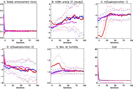
Fig. 2. Parameters converging in two identical twin tests for 1 and 5 year iteration, with
different starting points. Red, dark blue and magenta lines indicate different experiments
with 1, 1 and 5 year iterations respectively. Thick lines represent ensemble means, thin
dashed lines indicate ensemble width (1 standard deviation). Cyan dotted lines indicate
parameter values used to generate synthetic data set.
22
Fig. 2. Parameters converging in two identical twin tests for 1 and 5 year iteration, with different starting points. Red, dark blue and magenta lines indicate different experiments with 1, 1 and 5 year iterations respectively. Thick lines represent ensemble means, thin dashed lines indicate ensemble width (1 standard deviation). Cyan dotted lines indicate parameter values used to generate synthetic data set.
loading was improved to around 90% and the same integra-tion length only required 15 h, however in our experiments convergence of this system required more model-years in to-tal resulting in a longer overall integration time. Computing resources were not a limiting factor and the performance of our system may be some way from optimal. Further investi-gation may be worthwhile for application to more computa-tionally demanding models.
We chose 5 parameters to tune using this system, identi-fied via some preliminary sensitivity analyses which involved a series of 10-year integrations in which 29 tunable param-eters were varied individually, within ranges believed to be physically reasonable (with the other parameters held fixed at the default values). The tunable parameters were from the radiation, convection, and surface parameterisations. The 5 variables finally selected were those which were found to have most effect on a skill score which was determined by the quality of fit to the tuning targets of December–January– February (DJF) and June–July–August (JJA) surface air tem-perature and precipitation (4 two-dimensional data sets in to-tal). The parameters selected were (A) a non-dimensional linear multiplier of the sensible and latent heats, (B) the convective precipitation rate in mm/day at which convective clouds start to form, (C) the large-scale cloud supersatura-tion for the liquid water path calculasupersatura-tion, (D) the convective cloud supersaturation for the liquid water path calculation,
and (E) the relative humidity at which large-scale clouds are assumed to completely cover a grid-box. Three of the pa-rameters (B, C, and D) are constrained to be positive, but can otherwise vary by several orders of magnitude without inval-idating the model. For these, we use a logarithmic transfor-mation as in Annan et al. (2005), in order to avoid negative analysis values. The remaining two parameters (A and E) have a priori much more restricted ranges and therefore no transformation was necessary.
3 Identical twin testing
3.1 Experimental details
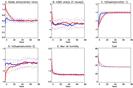
Fig. 3. Parameters converging in two experiments with reanalysis data (red and dark blue
lines as for Fig. 2).
23
Fig. 3. Parameters converging in two experiments with reanalysis data (red and dark blue lines as for Fig. 2).
This is because the short model integrations used in the iter-ative scheme will have a correspondingly larger component of chaotic noise, and so it is not possible for them even in principle to match the observed values to within this obser-vational accuracy. Attempting to fit the data more closely than is possible, forces the ensemble to collapse to a point in parameter space. Moreover, the spatial correlation of the model bias implies that the observational errors are not truly independent. Therefore, the error statistics were scaled up by a somewhat arbitrary factor of 20, the influence of which was checked by comparing the posterior model skill to the ex-pected value for a short integration with correct parameters. Clearly this ad-hoc adjustment is not an entirely satisfactory approach and further investigations are planned. The errors were also assumed spatially invariant.
The ensemble was initialised with each member having parameters chosen from a distribution some way removed from the truth run. Since the spin-up time of the model is so fast, there is no systematic dependence of the climatology on the initial fields even for a 1 year integration. Furthermore, the model appears to have a problem when initialised with an excessively cold state in the polar regions (which can arise in some analysed model states), so rather than attempting to corect this problem here we instead decided to re-initialise from a uniform state (“cold start”) rather than use the anal-ysed model fields throughout the iterative analysis procedure. Obviously, for a model with a longer spin-up time,
compu-tational efficiency would be improved by using the analysed state which should be in reasonable balance with the anal-ysed parameter set.
There are two primary adjustable controls on our assimila-tion scheme, being the length of integraassimila-tion between analysis steps, and the ensemble inflation factor. A longer integration interval gives more stable estimates of each ensemble mem-ber’s climatology, with the noise due to deterministic chaos decreasing in inverse proportion to the square root of the run length, as if it was truly random noise (Lea et al., 2000). A larger ensemble inflation factor also gives more rapid conver-gence but is potentially less accurate in nonlinear situations. In practice, run lengths of 1 and 5 years, with an inflation factor of 10%, gave good results which are now described further.
3.2 Identical twin results
J. D. Annan et al.: Parameter estimation in an atmospheric GCM using the Ensemble Kalman Filter 369
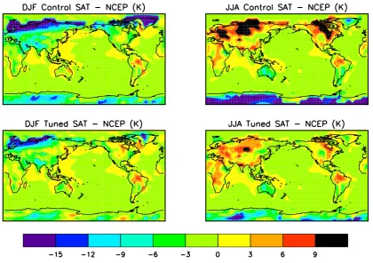
Fig. 4. Model SAT errors (degrees Kelvin), before and after tuning.
24
Fig. 4. Model SAT errors (degrees Kelvin), before and after tuning.distributions, consistent with the truth. Parameter D is not so clear, with perhaps some evidence of a continued mod-est drift to lower values, but again it is consistent with the value used to generate the identical twin data. Parameter B, however, is clearly not constrained in the 1 year experiments although there are some signs that it is converging with the 5 year iterations. Given that these parameters were initially selected to be those for which the model was most sensi-tive, this suggests that the data used are barely adequate for constraining as many as 5 parameters simultaneously. Even though there are 8196 data points in all, they only represent 2 types of measurement so this is a not entirely unexpected result. It is, however, also possible that the preselection of sensitive parameters (based around the default values) may not be valid close to this new optimum.
The cost function of an ensemble member is given by the sum of the squared differences between model and synthetic data fields, normalised by the number of model grid points. The cost function line plotted in Fig. 2 is the mean of the costs of the ensemble members (rather than the cost of their mean output). A typical cost of a little over 7 in the pos-terior ensemble for the 1 year iterations is made up of 5.5 for the two temperature fields (√5.5/2=1.4 K RMS error at each gridpoint) and 1.6 for the precipitation (0.9 mm/d RMS precipitation error). This is essentially the same as the vari-ability between model runs due to stochastic noise. For the 5 year integration, the cost is about 2, illustrating not a superior solution (the parameter distributions are essentially the same)
but the effect of the longer integration on reducing the magni-tude of the deterministic noise. At the true parameter values and arbitrary initial conditions, stochastic noise generates a cost of 1.7, so the range of parameter values in the posterior distribution is generating a marginally worse fit to the data than that due to stochastic noise alone. All ensembles have generated similar parameter distributions despite the differ-ent experimdiffer-ental conditions. This suggests that multiple lo-cal minima are not a significant problem in this application, if they exist at all.
4 Application using reanalysis data
We now apply the method using observational data. The sur-face air temperature and the precipitation both come from climatological monthly-mean NCEP reanalysis.
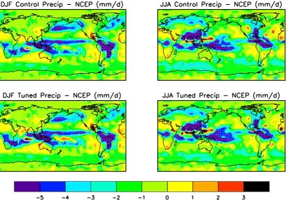
Fig. 5. Model precipitation error (mm/d), before and after tuning.
25
Fig. 5. Model precipitation error (mm/d), before and after tuning.forced to the edges of their ranges, there were fewer remain-ing effective degrees of freedom and less nonlinearity in the parameter space. Again, repeat runs under different condi-tions did not find any different solucondi-tions. Figure 3 shows the evolution of the parameter distributions and cost functions for two experiments.
The ensemble mean temperature matches the data fairly well (Fig. 4), with a typical RMS error of 3K at each grid-point. However, it should be noted that in tuning to reanalysis data, we have chosen a somewhat easier target than if we had used pure observations. Substantial cold biases over the high plateaux (especially Tibet) are present in almost all AGCMs, including that used for the NCEP reanalysis. This compari-son therefore gives an optimistic impression of model skill by masking the same failing in our model. In contrast to the rea-sonable temperature fields, precipitation remains poor in all simulations (Fig. 5), with an RMS error as high as 3mm per day. In fact, even attempting to tune to precipitation alone, completely ignoring the fit to the temperature data, did not improve that result. The model parameters appear to have very little effect on precipitation patterns, despite several of them relating directly to hydrology. Re-examining the re-sults from the univariate sensitivity analysis indicated that the wider range of 29 parameters tested all had a minimal effect on the precipitation. Disabling the convection scheme entirely, changed the model precipitation more substantially (and in fact led to an overall improvement). Clearly this points to a significant structural deficiency and research is
now under way to investigate alternative convection schemes. Although the model output is disappointing in this respect, the power of this multivariate tuning method is still appar-ent here in efficiappar-ently and rigorously idappar-entifying the limit of the parameter tuning and thereby motivating investigation of structural changes which are now under way.
The overall fit to the data, using our unweighted cost func-tion, dropped from a value of 78 for the default parameters, to 33 for the tuned ensemble, representing an improvement of about 1−√33/78=35% in the typical model-data mismatch.
5 Conclusions
J. D. Annan et al.: Parameter estimation in an atmospheric GCM using the Ensemble Kalman Filter 371 proved its worth by showing that parameter tuning will not
improve this aspect of model behaviour, and we expect it to contribute futher in the creation of the coupled atmosphere-ocean model. With more data sources, there are no obvious reasons why many more parameters could not be simultane-ously tuned as the computational time appears to only scale slowly with the number of free parameters.
Although the model as presented here is not directly suited to climate prediction (being created as one component of an Earth system model), the success of the method in this appli-cation strongly suggests that there are no fundamental rea-sons why future applications to prediction using more com-plete models should not be successful.
Acknowledgements. Supercomputer facilities and support were
provided by JAMSTEC. This research was partly supported by both the GENIE project (http://www.genie.ac.uk/), which is funded by the Natural Environment Research Council (NER/T/S/2002/00217) through the e-Science programme, and the NERC RAPID pro-gramme.
Edited by: S. Vannitsem Reviewed by: two referees
References
Allen, M.: Do it yourself climate prediction, Nature, 401, 642, 1999.
Allen, M., Kettleborough, J., and Stainforth, D.: Model er-ror in weather and climate forecasting, in Proceedings of the 2002 ECMWF predictability seminar,ECMWF, Reading, United Kingdom, 275–294, 2002.
Anderson, J. L.: An ensemble adjustment Kalman filter for data assimilation, Monthly Weather Review, 129, 2884–2902, 2001. Annan, J. D. and Hargreaves, J. C.: Efficient parameter estimation
for a highly chaotic system, Tellus, 56A, 520–526, 2004. Annan, J. D., Hargreaves, J. C., Edwards, N. R., and Marsh, R.:
Parameter estimation in an intermediate complexity Earth Sys-tem Model using an ensemble Kalman filter, Ocean Modelling, 8, 135–154, 2005.
Bellman, R.: Adaptive Control Processes: A Guided Tour, Prince-ton University Press, 1961.
de Forster, P. M., Blackburn, M., Glover, R., and Shine, K. P.: An examination of climate sensitivity for idealised climate change experiments in an intermediate general circulation model, Cli-mate Dynamics, 16, 833–849, 2000.
Derber, J.: A variational continuous assimilation scheme, Monthly Weather Review, 117, 2437–2446, 1989.
Edwards, N. R. and Marsh, R.: Uncertainties due to transport-parameter sensitivity in an efficient 3-D ocean-climate model, Climate Dynamics, in press, 2005.
Evensen, G.: Sequential data assimilation with a nonlinear quasi-geostrophic model using Monte Carlo methods to forecast error statistics, J. Geophys. Res., 99, 10 143–10 162, 1994.
Evensen, G.: The ensemble Kalman filter: theoretical formulation and practical implementation, Ocean Dynamics, 53, 343–367, 2003.
Evensen, G. and Leeuwen, P. J. V.: An Ensemble Kalman Smoother for nonlinear dynamics, Monthly Weather Review, 128, 1852– 1867, 2000.
Giorgi, F. and Mearns, L.: Calculation of average, uncertainty range, and reliability of regional climate changes from AOGCM simulations via the “reliability ensemble averaging” (REA) method, Journal of Climate, 15, 1141–1158, 2002.
Hargreaves, J. C., Annan, J. D., Edwards, N. R., and Marsh, R.: Cli-mate forecasting using an intermediate complexity Earth System Model and the ensemble Kalman filter, Climate Dynamics, 23, 745–760, 2004.
Highwood, E. J. and Stevenson, D. S.: Atmospheric impact of the 1783-1784 Laki eruption. Part II - Climatic effect of sulphate aerosol, Atmos. Chem. Phys., 3, 1177—1189, 2003,
SRef-ID: 1680-7324/acp/2003-3-1177.
Joshi, M., Shine, K., Ponater, M., Stuber, N., Sausen, R., and Li, L.: A comparison of climate respone to different radiative forcings in three general circulation modles: towards an improved metric of climate change, Climate Dynamics, 20, 843–854, 2003. Kalman, R. E.: A new approach to linear filtering and prediction
problems, J. Basic Engineering, 82D, 33–45, 1960.
Keppenne, C. L.: Data assimilation into a primitive-equation model with a parallel ensemble Kalman filter, Monthly Weather Review, 128, 1971–1981, 2000.
Kivman, G. A.: Sequential parameter estimation for stochastic sys-tems, Nonlin. Proc. Geophys., 10, 253–259, 2003,
SRef-ID: 1607-7946/npg/2003-10-253.
Knutti, R., Stocker, T. F., Joos, F., and Plattner, G.-K.: Constraints on radiative forcing and future climate change from observations and climate model ensembles, Nature, 416, 719–723, 2002. K¨ohl, A. and Willebrand, J.: An adjoint method for the
assimila-tion of statistical characteristics into eddy-resolving ocean mod-els, Tellus, 54A, 406–425, 2002.
K¨ohl, A. and Willebrand, J.: Variational assimilation of SSH variability from TOPEX/POSEIDON and ERS1 into an eddy-permitting model of the North Atlantic, Journal of Geophysical Research, C3, art. num. 3092, 2003.
Lea, D. J., Allen, M. R., and Haine, T. W. N.: Sensitivity analysis of the climate of a chaotic system, Tellus, 52A, 523–532, 2000. Lea, D. J., Haine, T. W. N., Allen, M. R., and Hansen, J. A.:
Sensi-tivity analysis of the climate of a chaotic ocean circulation model, Q. J. R. Meteorological Soc., 128, 2587–2605, 2002.
Losa, S. N., Kivman, G. A., Schr¨oter, J., and Wenzel, M.: Sequen-tial weak constraint parameter estimation in an ecosystem model, Journal of Marine Systems, 43, 31–49, 2003.
Murphy, J. M., Sexton, D. M. H., Barnett, D. N., Jones, G. S., Webb, M. J., Collins, M., and Stainforth, D. A.: Quantification of mod-elling uncertainties in a large ensemble of climate change simu-lations, Nature, 430, 768–772, 2004.
Nozawa, T., Emori, S., Numaguti, A., Tsushima, Y., Takemura, T., Nakajima, T., Abe-Ouchi, A., and Kimoto, M.: Projections of Future Climate Change in the 21st Century Simulated by the CCSR/NIES CGCM under the IPCC SRES Scenarios, in Present and Future of Modeling Global Environment Change, edited by: Matsuno, T. and Hideji, K., Terra Scientific Publishing Company, 15–28, 2001.
Pisarenko, V. F. and Sornette, D.: Statistical methods of parame-ter estimation for deparame-terministically chaotic time series, Physical Review E, 69, 036122, 2004.
Press, W. H., Teukolsky, S. A., Vetterling, W. T., and Flannery, B. P.: Numerical recipes in Fortran: the art of scientific com-puting, Cambridge University Press, 1994.