https://doi.org/10.5194/tc-11-2847-2017
© Author(s) 2017. This work is distributed under the Creative Commons Attribution 4.0 License.
Snowmelt response to simulated warming across a large elevation
gradient, southern Sierra Nevada, California
Keith N. Musselman1,a, Noah P. Molotch2,3, and Steven A. Margulis4
1National Center for Atmospheric Research, Boulder, CO, USA
2Department of Geography, Institute of Arctic and Alpine Research, University of Colorado, Boulder, CO, USA 3Jet Propulsion Laboratory, California Institute of Technology, Pasadena, CA, USA
4Department of Civil and Environmental Engineering, University of California, Los Angeles, CA, USA anow at: Institute of Arctic and Alpine Research, University of Colorado, Boulder, CO, USA
Correspondence:Keith N. Musselman ([email protected]) Received: 29 June 2017 – Discussion started: 18 July 2017
Revised: 16 October 2017 – Accepted: 27 October 2017 – Published: 11 December 2017
Abstract.In a warmer climate, the fraction of annual melt-water produced at high melt rates in mountainous areas is projected to decline due to a contraction of the snow-cover season, causing melt to occur earlier and under lower energy conditions. How snowmelt rates, including extreme events relevant to flood risk, may respond to a range of warming over a mountain front is poorly known. We present a model sensitivity study of snowmelt response to warming across a 3600 m elevation gradient in the southern Sierra Nevada, USA. A snow model was run for three distinct years and ver-ified against extensive ground observations. To simulate the impact of climate warming on meltwater production, mea-sured meteorological conditions were modified by +1 to
+6◦C. The total annual snow water volume exhibited lin-ear reductions (−10 %◦C−1)consistent with previous stud-ies. However, the sensitivity of snowmelt rates to successive degrees of warming varied nonlinearly with elevation. Mid-dle elevations and years with more snowfall were prone to the largest reductions in snowmelt rates, with lesser changes sim-ulated at higher elevations. Importantly, simsim-ulated warming causes extreme daily snowmelt (99th percentiles) to increase in spatial extent and intensity, and shift from spring to winter. The results offer insight into the sensitivity of mountain snow water resources and how the rate and timing of water avail-ability may change in a warmer climate. The identification of future climate conditions that may increase extreme melt events is needed to address the climate resilience of regional flood control systems.
1 Introduction
Seasonal snow accumulation and melt in mountainous ar-eas are critical components of the regional hydrologic cy-cle with important controls on climate, ecosystem function, flood risk, and water resources (Bales et al., 2006; Barnett et al., 2005). Warmer temperatures are expected to reduce snowpack volume and persistence (Gleick, 1987; Knowles and Cayan, 2004; Mote et al., 2005) by shifting precipitation from snowfall to rain (Knowles et al., 2006) and causing ear-lier snowmelt (Stewart et al., 2004). Studies of historical ob-servations in the western USA have identified recent declines in spring snowpack (Mote et al., 2005), diminished snowmelt runoff volumes (Dettinger and Cayan, 1995; McCabe and Clark, 2005), and earlier spring runoff (Stewart et al., 2004). Most of these studies have attributed the observed trends to anomalously warm spring and summer temperatures of re-cent decades. Fyfe et al. (2017) report that the rere-cent snow-pack declines are not replicable with climate model simula-tions forced by natural changes alone, but are resolved when both natural and anthropogenic changes are considered.
et al., 2004; Godsey et al., 2013; Knowles and Cayan, 2002; Lettenmaier and Gan, 1990). It is not well understood how present-day snowmelt rates may respond to the range of pro-jected warmer temperature scenarios and, particularly, how those changes will impact water availability over large eleva-tion gradients.
Elevation is a dominant explanatory variable of moun-tain snow-cover persistence (Girotto et al., 2014b), ranking in importance above solar radiation and terrain aspect for many basins in the western USA (Molotch and Meromy, 2014). Snowpack response to warmer temperatures exhibits strong nonlinear elevation dependencies (Brown and Mote, 2009; Knowles and Cayan, 2004). For example, slight warm-ing can cause drastic hydrologic response at lower eleva-tions as rain becomes the predominant hydrologic input and snow cover becomes seasonally intermittent or negligible (Hunsaker et al., 2012; Marty et al., 2017; Nolin and Daly, 2006). At higher and cooler elevations, snowmelt may re-main a substantial component of the annual hydrologic in-put in a warmer climate, but the timing and rate of melt are altered. Rapid and prolonged spring snowmelt is unique to these mountain environments (Trujillo and Molotch, 2014). This efficient runoff generation mechanism (Barnhart et al., 2016) produces water resources of vast economic impor-tance (Sturm et al., 2017). Improved understanding of re-gional elevation-dependent snowmelt response to warming is a key step toward better predicting and interpreting model estimates of basin-wide runoff.
In a warmer climate, the fraction of meltwater produced at high melt rates is projected to decrease due to a con-traction of the historical melt season to a period of lower available energy (Musselman et al., 2017). Because stream-flow is a nonlinear response to hydrologic input, slight re-ductions in snowmelt rates may disproportionately reduce runoff. Despite recent advances in process understanding, the sensitivity of snowmelt rates to a range of potential warm-ing over a foothills-to-headwaters elevation profile remains poorly known. The topic is a key determinant of changes in how precipitation is partitioned amongst soil storage, evap-otranspiration, and runoff, with implications for ecological response (Tague and Peng, 2013; Trujillo et al., 2012) and regional water resources (Gleick and Chalecki, 1999; Vano et al., 2014).
We present a climate sensitivity experiment to investigate how carefully verified model simulations of historical snow water equivalent (SWE) and melt rates respond to succes-sively warmer temperatures that span the range of projected wintertime warming over western North America for this century (Van Oldenborgh et al., 2013). A controlled exper-iment with a physically based snow model promotes a de-tailed analysis of the following research questions: (1) how do SWE and snowmelt rates vary with elevation and how do those gradients vary amongst dry, average, and wet snow seasons? (2) How do historical SWE and snowmelt rates re-spond to successive degrees of warming?
2 Methods
To evaluate the response of SWE and snowmelt dynamics to warmer temperatures, we conduct a reanalysis of historical snow seasons using the physically based Alpine3D (Lehn-ing et al., 2006) snow model run at 100 m grid spac(Lehn-ing over a mountainous region spanning a 3600 m elevation gradient in the southern Sierra Nevada, California. Snowpack simu-lations for three historical snow seasons were first verified against multi-scale, ground-based observations. Simulated snowpack characteristics over discrete elevation bands were then examined for their sensitivity to warmer conditions us-ing a delta-change approach in which observed air tempera-ture values and the longwave radiative equivalent were aug-mented by+1 to+6◦C in+1◦C increments. Given the rela-tively small (< 10 %) precipitation changes projected for cen-tral and southern California (Cayan et al., 2008), and a lack of agreement of climate models on the sign of projected pre-cipitation changes (Seager et al., 2013), the focus of the cur-rent study is on the snowpack response to simulated warming rather than combined changes in temperature and precipita-tion. Sensitivity was examined for three historical snow years representative of the climatological range in snowfall (years with below-average, average, and above-average snowfall), snow-cover duration, and precipitation timing. The following sub-sections describe the details of our model experiment, verification, and analysis methods.
2.1 Study domain
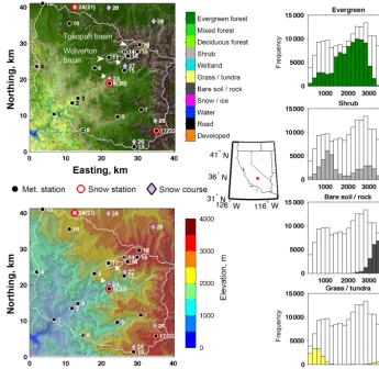
Figure 1.The elevation and land cover distribution of the model domain encompassing the Kaweah River basin (outlined) on the western side of the southern Sierra Nevada, California. Locations of the forested Wolverton and largely alpine Tokopah research basins are indicated. The locations of 19 automated meteorological stations (filled circle markers), three automated snow stations (red circles), and seven monthly snow survey transects (diamond markers) are shown. Station numbers correspond to those in Table 1. The histograms illustrate the elevation distribution of the four primary land cover types (colored bars) relative to the elevation of the model domain (empty bars).
with sparse alpine vegetation and snow cover typically per-sists from November to July.
The domain includes two research basins: the 7.22 km2 forested Wolverton basin and the 19.1 km2 largely alpine Tokopah basin (Fig. 1). The Wolverton basin is representative of regional forested mid-elevations. A detailed description of the Wolverton basin instrumentation is provided in Mus-selman et al. (2012b). The 19.1 km2 Tokopah basin is rep-resentative of regional small headwater basins (Tonnessen, 1991). It is instrumented with numerous meteorological sta-tions and has been the subject of many studies on snow dis-tribution (Elder et al., 1988; Girotto et al., 2014a; Jepsen et al., 2012; Marks et al., 1992; Molotch et al., 2005) and biogeochemistry (Perrot et al., 2014; Sickman et al., 2003; Williams and Melack, 1991). We use ground-based observa-tions from these research basins to verify the model as de-scribed in Sect. 2.4.
2.2 Snow model
uncal-Table 1.Meteorological station and snow measurement details. Station numbers are ranked by station elevation and correspond to those mapped in Fig. 1. The variables measured at each location are listed: air temperature (Ta), relative humidity (RH), wind speed (ws),
precipi-tation (ppt), snow water equivalent (SWE), and snow depth (depth).
No. Station name Elev., m Measured variables* Operating agency**
Automated met. stations
1 D0117 263 Ta, RH, ws APRSWXNET
2 C4177 378 Ta, RH, ws APRSWXNET
3 Ash Mountain 527 Ta, RH, ws, ppt NPS
4 Shadequarter 1323 Ta, RH, ws CDF
5 Wolverton 1598 Ta, RH, ws NPS
6 Lower Kaweah 1926 Ta, RH, ws, ppt NPS
7 Atwell 1951 ppt USACE
8 Case Mountain 1967 Ta, RH, ws BLM
9 Giant Forest 2027 Ta, ppt USACE
10 Bear Trap Meadow 2073 ppt USACE
11 Wolverton Meadow 2229 Ta, RH, ws SNRI
12 Park Ridge 2299 Ta, RH, ws NPS
13 Hockett Meadows 2592 ppt USACE
14 Marble Fork 2626 Ta ERI
15 Panther Meadow 2640 Ta, RH, ws SNRI
16 Emerald Lake 2835 Ta, RH, ws ERI
17 Farewell Gap 2896 Ta USACE
18 Topaz Lake 3232 Ta, RH, ws, SW, LW ERI
19 M3 3288 Ta, RH, ws ERI
Automated snow stations
20 Giant Forest 1951 SWE USACE
21 Big Meadows 2317 SWE USACE
22 Farewell Gap 2896 SWE, depth USACE
Monthly snow courses
23 Giant Forest 1951 SWE, depth NPS
24 Big Meadows 2317 SWE, depth CADWP
25 Mineral King 2439 SWE, depth NPS
26 Hockett Meadow 2592 SWE, depth NPS
27 Panther Meadow 2622 SWE, depth NPS
28 Rowell Meadow 2698 SWE, depth KRWA
29 Scenic Meadow 2942 SWE, depth KRWA
* Meteorological variables used in this study.
* Agency abbreviations: APRSWXNET: Automatic Position Reporting System as a Weather NETwork; NPS: National Park Service (Sequoia and Kings Canyon National Parks); CDF: California Department of Forestry; USACE: United States Army Corps of Engineers; BLM: Bureau of Land Management; SNRI: Sierra Nevada Research Institute, University of California Merced; ERI: Earth Research Institute, University of California Santa Barbara; CADWP: California Department of Water and Power; KRWA: Kaweah River Water Association.
ibrated. Model decisions and parameters were chosen based on their successful application in previous studies.
The bottom (soil) boundary conditions were treated with a constant geothermal heat flux of 0.06 W m−2applied at the base of a six-layer soil module (see Musselman et al., 2012a). In the case of vegetation cover, the surface–atmosphere boundary conditions were solved for in a single-layer canopy module (Musselman et al., 2012a). Wind transport of snow is not considered in this model implementation. New-snow density and snow albedo parameterizations used in previ-ous studies in the European Alps (Bavay et al., 2013) were
2.3 Model input data
2.3.1 Topography and land-cover data
The elevation and land-cover across the domain were rep-resented at 100 m grid spacing. Land-cover classification (Fig. 1) was specified from the National Land Cover Database (NLCD; Fry et al., 2011). In addition to the land-cover classes listed in Fig. 1, forest-land-covered grid cells were aggregated into coniferous, mixed, and deciduous categories based on the dominant species within each cell. The NLCD canopy density values, used to parameterize canopy snow interception and snow surface energy fluxes, were binned from 5 to 85 % in 10 % intervals. Grid elements contain-ing vegetation were specified to have an effective leaf area index and canopy height, respectively, of 0.5 m2m−2 and 1.5 m for shrub/chaparral, 1.2 m2m−2 and 20 m for decid-uous, 2.0 m2m−2and 30 m for mixed, and 2.7 m2m−2and 40 m for coniferous forests.
2.3.2 Meteorological data
Hourly meteorological observations were available from 19 stations within the domain (Fig. 1 and Table 1). Sixteen sta-tions recorded hourly air temperature and six reported pre-cipitation (Table 1). The Ash Mountain station at 527 m a.s.l. provided the only low-elevation precipitation measurements. The Lower Kaweah, Atwell, Giant Forest, and Bear Trap Meadow stations are located within a narrow elevation band of 1926 to 2073 m a.s.l. (Fig. 1 and Table 1). Data from a single higher station (Hockett Meadow; 2592 m a.s.l.) were not used because of gauge error for the time period of inter-est. Precipitation gauge catch efficiency was specified as 0.95 for rain and 0.6 for snow, using the 1.2◦C air temperature threshold as a determinant of precipitation phase. Incoming shortwave radiation was provided from the Topaz Lake mete-orological station (Fig. 1; Table 1). The direct beam was ad-justed for grid-cell-specific terrain shading and elevation de-pendency and the diffuse component was assumed spatially uniform for each time step (see Bavay et al., 2013 for details). The shortwave radiation data are well correlated with mea-surements at middle elevations (Musselman et al., 2012b) and are used to model the full domain.
The remaining meteorological variables required spatial interpolation from station locations to all grid cells. Because elevation can have a profound influence on many of the me-teorological variables, several of the interpolation methods used linear elevation trends. Interpolations were conducted with the data access and pre-processing library MeteoIO (Bavay and Egger, 2014) and computed with an inverse dis-tance weighting (IDW) algorithm with elevation lapse rate adjustments for air temperature, wind speed, and precipita-tion. Lapse rates were computed for each hourly time step us-ing a regression technique (Bavay and Egger, 2014) applied to observations from all available stations. If the correlation
coefficient was less than 0.6, then a constant elevation lapse rate of−0.008◦C m−1was used for air temperature, and a
standardized elevation trend of 0.0006 m−1was used for
pre-cipitation. The incoming longwave radiation measured at the Topaz Lake station was distributed to all grid cells with a constant elevation lapse rate of−0.03125 W m−2m−1as in Bavay et al. (2013). Relative humidity was interpolated as in Liston and Elder (2006). The sensitivity of Alpine3D re-sults to meteorological interpolation and model decisions are addressed in Schlögl et al. (2016).
2.4 Snow observations and validation data
2.4.1 Seasonal basin-scale snow surveys
Snow surveys were conducted in the two research basins for three snow seasons: 2008, 2009, and 2010. Three snow sur-veys of the forested Wolverton basin were conducted each in 2008 and 2009. The survey timing coincided with peri-ods of accumulation (mid-February), maximum accumula-tion (mid-March), and melt (late April). In all three years, early April surveys of the alpine Tokopah basin were con-ducted. In 2009, two additional Tokopah basin surveys cap-tured accumulation (early March) and melt (mid-May). Sur-veys were conducted with graduated probes to measure snow depth at waypoint locations on a 250 m grid. Surveyors nav-igated to the waypoints using GPS units. At each waypoint, three snow depth measurements separated by 5 m were made along a north–south axis. In total over the 3 years, 1494 way-points were surveyed. During each survey, snow density was recorded from snow pits conducted at lower and upper ele-vations to capture the basin range of snow density; only one snow pit was dug during the 2010 Tokopah survey. An undis-turbed snow face was excavated to ground and snow density in duplicate columns was measured in 10 cm vertical inter-vals by weighing snow samples acquired with a 1000 cm3 cutter. In total, 26 snow pits were measured over the 3 years. The average snow density at all pits made during a survey was used to estimate SWE at waypoint locations, which rep-resent the average of three depth measurements. This ap-proach assumes that basin-scale snow density varies less than snow depth (López-Moreno et al., 2013).
Simulated SWE at model grid elements containing way-point positions are evaluated against the snow survey values. Three model evaluation metrics are reported. The model bias is computed as the average difference (“modeled minus mea-sured”) ofnsurvey measurements for each waypoint mea-surement SWEoi and corresponding model grid cell SWEmi. The root-mean-square error (RMSE) is computed as
RMSE= v u u t
1 n
n
X
i=1
SWEmi−SWEoi
2
and the normalized mean square error (NMSE) value is com-puted as
NMSE=(SWEm−SWEo) 2
SWEmSWEo
, (2)
where the over bars denote the mean over all waypoint loca-tions. The NMSE metric facilitates model performance com-parisons amongst basins, months, and years.
2.4.2 Monthly plot-scale snow surveys
Monthly (1 February–1 May) manual SWE measurements in the Sierra Nevada are made by the California Cooperative Snow Survey (CCSS) program to monitor regional water re-sources. Seven snow course sites are located within the study domain (Table 1); the sites range in elevation from 1951 to 2942 m. At each snow course, linear transects of approxi-mately 10 SWE measurements made with Federal snow tube samplers are averaged to represent the mean SWE over a dis-tance similar to the 100 m grid cell spacing. The survey mea-surements thus provide a SWE estimate that is arguably more representative of the average value within a corresponding model grid cell than the three point-measurements of the basin-scale surveys or a single automated SWE station mea-surement. Modeled SWE values for each survey date at the grid cells corresponding to each snow course location were evaluated against measured values.
2.4.3 Automated snow depth sensor network
In addition to the repeated basin- and plot-scale manual snow surveys, the Wolverton basin includes a network of 24 ultra-sonic snow depth sensors. Four research sites at different el-evations (2253, 2300, 2620, and 2665 m a.s.l.) each include six snow depth sensors and each site falls within a differ-ent 100 m×100 m model grid cell. The range of snow depth measured at the six sensors provides a robust estimate of the snow depth, and thus model skill, at four grid cells spanning slope, aspect, forest density, and elevation in the basin. 2.4.4 Automated SWE stations
Daily SWE observations were available from three CCSS au-tomated stations (i.e., snow “pillows”) at middle elevations: Giant Forest (1951 m a.s.l.), Big Meadows (2317 m a.s.l.), and Farewell Gap (2896 m; Table 1 and Fig. 1). Modeled SWE fields were evaluated against these station observations using the RMSE and bias metrics described above. The cli-matological mean SWE record (26 years at Giant Forest and Big Meadows; 15 years at Farewell Gap) was used to evalu-ate how the three snow seasons studied here compare to the long-term average.
2.5 Experimental design
The model was run to simulate seasonal snow dynamics for three reference water years (1 October 2007–30 September 2010) for which the extensive ground-based observations were available. Model estimates of snow depth and SWE were evaluated against the observations.
Six warmer temperature scenarios for each of the three ref-erence years were simulated by increasing the hourly mea-sured air temperature from the 19 regional meteorological stations by +1 to +6◦C in 1◦C increments. The lower (+1◦C) and upper (+6◦C) limits of simulated warming cor-respond to the average winter air temperature increases pro-jected for the year 2100 in western North America in the Representative Concentration Pathway (RCP) emissions sce-narios 2.6 (lowest emissions) and 8.5 (highest emissions), respectively (see top-right panel in Fig. A1.16 in Van Old-enborgh et al., 2013). For each warmer temperature scenario (+n◦C) and hourly time step (t), the incoming longwave ra-diation LW↓t (W m−2) measured at the Topaz Lake station
was adjusted for the increase in effective radiative tempera-ture resulting from the warmer air. The in situ atmospheric emissivityt was estimated from the hourly air temperature
Tat (
◦C):
t=
LW↓t
σ (Tat+273.15)4
, (3)
where σ is the Stefan–Boltzmann constant (5.670373×
10−8W m−2K−4). The longwave radiation was adjusted for an effective radiative temperature increase ofn(◦C) as LW↓t(Ta+n)=tσ (Tat+273.15+n)
4. (4)
Relative humidity was held constant to allow water vapor pressure to vary in a manner consistent with the ideal gas law (Rasouli et al., 2015). The in situ atmospheric emissiv-ity is assumed to be constant for the perturbed temperature scenarios. A lack of clear projected wintertime precipitation response to climate change in the southern Sierra Nevada (see Fig. A1.18 in Van Oldenborgh et al., 2013) prompted our focus on temperature sensitivity rather than a combina-tion of temperature and precipitacombina-tion. Observed and adjusted meteorological variables representative of the warmer sce-narios were interpolated to domain grid cells as described in Sect. 2.3.2. The model was run as in the reference scenarios (Sect. 2.2).
snowmelt (hereafter, snowmelt rate). The total annual melt-water is then the annual sum of daily snowmelt.
To evaluate how SWE and melt in each scenario varied with elevation, metrics were averaged or summed into 200 el-evation bands, each encompassing∼18 vertical meters, with a mean of 823 grid cells per elevation band (maximum of 1412). Rice et al. (2011) found that snow disappearance in the Sierra Nevada occurred 20 days later for each 300 m rise in elevation. The 18 m elevation discretization captures this variability at approximately 1 day per elevation band. For each warmer scenario, the total annual meltwater volume is reported as the fraction of that simulated in the nominal (i.e., unperturbed) case. For all scenarios, we report the annual meltwater in three ways: the average meltwater volume and melt rate within each elevation band, the sum of annual water within each elevation band, and the total annual melt-water summed over the entire model domain. The sensitivity of total domain-wide annual meltwater to simulated warming is examined with a (linear) regression analysis of the fraction of historical total meltwater for each warmer scenario of the three years.
To evaluate the effect of simulated warming on melt rates over the elevation profile for the three years, we report the elevation-specific mean fraction of total annual melt-water produced at high (≥15 mm day−1) melt rates, re-ported as a percent change relative to the nominal case. The 15 mm day−1 threshold was selected as a compromise be-tween the 12.5 mm day−1 threshold above which positive streamflow anomalies were reported by Barnhart et al. (2016) and a 20 mm day−1 classification of very heavy rainfall (Klein Tank et al., 2009) used by Musselman et al. (2017). To examine how daily snowmelt rates respond to simulated warming, we present a quantile analysis of the 25th, 50th, 75th, 90th, 95th, and 99th percentiles of daily snowmelt rates
≥ 1 mm day−1from the warmer scenarios compared to those from the nominal case. For this analysis, the model domain was divided into three elevation bands: 1500 to 2250, 2250 to 2800, and > 2800 m a.s.l., and percentiles of daily snowmelt were computed for all grid cells in each elevation band. The analysis was conducted separately for each of the three wa-ter years and seven scenarios. Lastly, we present an analysis of the meteorological conditions that control the response of snowmelt rates to successive degrees of simulated warming.
3 Results
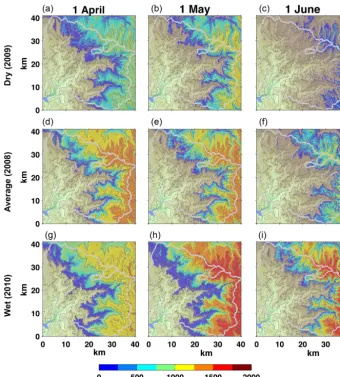
Maps of simulated SWE on 1 April, 1 May, and 1 June (Fig. 2) highlight seasonal and interannual SWE patterns and illustrate the great variability of SWE with elevation. The lowest elevations were consistently snow-free during the spring. Middle elevations included a transition zone from snow-free to seasonally persistent snow cover; that transi-tion occurred at progressively higher elevatransi-tions later in the melt season and occurred earlier (later) in the drier
(wet-Table 2.Average (hourly) air temperature and shortwave radiation values measured at the alpine Topaz Lake meteorological station in the Tokopah Basin for JFM and AMJ of the moderately dry year (2009), near-average year (2008), and moderately wet year (2010).
Air temperature,◦C Shortwave, W m−2
JFM AMJ JFM AMJ
2009 −3.2 3.3 163 279
2008 −3.6 3.4 166 317
2010 −4.0 1.3 152 306
ter) snow years. The upper elevations contained the great-est SWE and most persistent spring snow cover (Fig. 2). The 3-year observation period captured years with below-average snowfall (2009; 23 % below-below-average SWE; hereafter “moderately dry year”), average snowfall (2008; 7 % above-average SWE; hereafter “above-average year”), and above-above-average snowfall (2010; 54 % above-average SWE; hereafter “mod-erately wet year”) as determined from regional automated SWE records (Fig. 3 and Table S1 in the Supplement). The average (hourly) air temperature and shortwave radiation val-ues measured at the alpine Topaz Lake station in January– February–March (JFM; the accumulation season) and April– May–June (AMJ; the melt season) provide more insight into the meteorological differences amongst the three years. The drier and average years exhibited similar average air temper-atures, but the AMJ mean shortwave radiation was lower in the moderately dry year (Table 2) due to higher spring cloud-cover (see Fig. 6 in Musselman et al., 2012b). The AMJ pe-riod in the moderately wet year was > 2◦C colder than the other years (Table 2) due to a series of large snowfall events in mid-April (Fig. 3) that prolonged snow cover well into June (see Figs. 2 and 3). By comparison, snow cover mea-sured by the automated SWE stations generally disappeared in May in both the drier and average years (Fig. 3).
3.1 Model evaluation against observation
Compared to automated snow pillow SWE measurements, the model performed favorably (RMSE≤100 mm; bias bet-ter than±85 mm) at all elevations in 2008 and 2010 (Fig. 3). In 2009, the model underestimated SWE compared to mea-surements made at the two higher-elevation stations, but accurately simulated SWE at the lower Giant Forest sta-tion (RMSE=34 mm; bias= −4 mm; Fig. 3). The greatest model error occurred in 2009 at the Big Meadows station (2317 m a.s.l.) resulting from a significant underestimation of all snow events, possibly due to sensor error, and errors were less at the higher and lower-elevation stations in this year (Fig. 3).
dynam-Figure 2.Simulated SWE over the greater Kaweah River basin on the first of April(a, d, h), May(b, e, i), and June(c, f, j)for a moderately dry water year (2009;a, b, c), near-climatological-average water year (2008;d, e, f), and a moderately wet water year (2010;g, h, i).
ics, including maximum accumulation, the rate of depletion, and the date of snow disappearance (Fig. 4; note that simu-lated snow depth is generally within the measurement enve-lope). The underestimation of SWE in 2009 was not apparent in the verification against the six automated depth measure-ments at four sites in the Wolverton basin (Fig. 4).
The early April surveys of the alpine Tokopah basin show 2009, 2008, and 2010 being the drier (849±401 mm SWE), average (1000±476 mm SWE), and wetter (1265±310 mm SWE) snow seasons, respectively (Table S2). Model SWE er-rors (NMSE) were highest during the melt season when the measured variability was high relative to the mean, and low-est during the accumulation season (Table S2). On average, the forested Wolverton and alpine Tokopah basins exhibited similar NMSE values of∼0.14 at maximum accumulation. In general, the model tended to overestimate SWE with the exception of the February 2009 Wolverton survey, for which modeled SWE was negatively biased (Table S2). The survey
mean bias values were typically much less than the standard deviation of the biases.
In general, model SWE errors were lower when evalu-ated against the CCSS snow course measurements (Table S3) than the basin-wide survey measurements (Table S2). The large underestimation of SWE in 2009 seen in the compari-son against the automated SWE stations (Fig. 3) is also seen in comparison to SWE measured at the two lowest eleva-tion snow course sites (Table S3). Conversely, comparison to the two highest elevation snow course sites indicated a slight positive model bias in 2009. Overall, the model performed best in regions closest to precipitation gauges used to force the model; SWE RMSE values were better explained by this metric than by elevation alone (Fig. S1).
Figure 3. Measured and simulated SWE at the three automated snow stations spanning the middle elevations of the greater Kaweah River basin. The error metrics RMSE and bias, in millimeters, are provided for each station-year. The thin gray line indicates the long-term climatological mean SWE based on 26 years of data (1988– 2014) collected at the Giant Forest and Big Meadows stations and a 15-year record (2000–2014) at the Farewell Gap station.
the three years. Persistent seasonal snowpack was simulated > 1800 m a.s.l. in all years. Maximum annual SWE increased with elevation (colors in the top row panels of Fig. 5); how-ever, the date of maximum SWE exhibited a complex rela-tionship with elevation, snowfall magnitude and timing, and snowpack persistence that all varied amongst years (Fig. 5). Generally, maximum SWE occurred later with increasing el-evation but progressed in a step-wise manner, often with lit-tle change over hundreds of vertical meters interspersed with abrupt jumps of 1 to 2 months (Fig. 5; note the occasional large horizontal spacing between “X” markers of adjacent elevation bands).
Simulated daily melt was episodic in nature with the high-est rates (> 35 mm day−1; red in the bottom panels of Fig. 5) generally confined to elevations > 2000 m a.s.l. and the late spring and early summer. The highest elevations and years with more/later snow had the highest melt rates. In all three years, winter melt was generally low (< 5 mm day−1)with rare, episodic, and more intense melt events confined to lower elevations (Fig. 5).
3.3 Elevation-dependent snowpack and snowmelt response to warming
In the nominal case, the total meltwater volume summed over each elevation band was consistently greatest between
2500 m and 2800 m a.s.l. (see Fig. 6; right panels), corre-sponding to the peak in the regional hypsometry (see his-tograms in Fig. 1). Under the warmer scenarios, the maxi-mum meltwater volume, inferred from the peaks in Fig. 6, shifts upward in elevation by∼600 m to the regional tree line (see Fig. 1). This upward elevation shift occurred under
+2, +3, and +4◦C warming for the dry, average, and wet snow seasons, respectively. Additional warming reduced the total melt volume but did not change the elevation at which the maximum volume occurred.
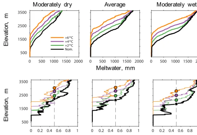
Lower and middle elevations were prone to large reduc-tions in the fraction of historical meltwater volume (see line graphs in Fig. 6). At 2000 m a.s.l., only 50 % of the historical water in the form of snow remained in a+3◦C scenario, fur-ther reducing to 20 % in the+5◦C scenario. Overall, snow at the upper elevations in the moderately dry snow season was more susceptible to large reductions (Fig. 6). Conversely, up-per elevation snowpack during the average and higher snow-fall seasons was more resilient to warming. For example, at 2700 m a.s.l.,+1◦C warming reduced annual meltwater vol-ume by 1, 3, and 11 % in the wetter, average, and drier snow seasons, respectively; those values increased to 7, 21, and 28 % in the+3◦C scenario.
Despite elevation-dependent nonlinear meltwater response to warming, the domain-total meltwater volume exhibited linear response to successive warming. Figure 7 shows lin-ear regressions fit to the fraction of the nominal-case total meltwater for each scenario and year (see Table S4). The dry and average years were slightly more susceptible to warm-ing (−10.5 to−10.8 % change per◦C) than the wetter year (−9.3 % change per◦C). Sublimation estimates ranged from 5 to 9 % in the nominal case to 8 to 14 % in the+6◦C sce-nario (Table S4).
Warmer temperatures impact not only the total annual meltwater, but also the rate at which meltwater is pro-duced. Figure 8 shows the fraction of the total meltwater per unit area over the elevation profile that is produced at high (≥15 mm day−1)melt rates; the complement of that fraction occurs at lower (< 15 mm day−1)rates. Consistently, meltwa-ter production at upper elevations is dominated by high melt rates, while at lower-elevations melt rates are predominately low. At∼2200 m a.s.l., melt in the nominal cases occurred equally at low and high rates; above this middle elevation zone, melt occurs at high rates (≥15 mm day−1)and at low rates (< 15 mm day−1)below this elevation (see black circle markers in Fig. 8). Warming greatly decreases the fraction of meltwater produced at high melt rates and increases that pro-duced at low rates (see lower colored graphs in Fig. 8). As a result, the elevation at which meltwater is produced equally at low and high rates is pushed upward by ∼150 m◦C−1 (Fig. 8). The greatest melt rate reductions occur at forested elevations with generally lesser change in alpine areas above
∼3300 m a.s.l.
2008
2009
2010
2253
m
2300
m
2620
m
2665
m
In
cr
ea
si
ng
e
le
va
ti
on
Sno
w
dep
th
cm
Sno
w
dep
th
cm
Obs. range Obs. mean Simulated
Figure 4.Comparison of three years (panel columns) of daily (xaxes) simulated (red lines) snow depth and the six-sensor observed range (gray lines) and mean (bold lines) snow depth measured by automated sensors at four research sites (panel rows) at different elevations in the Wolverton basin.
O N D J F M A M J J 500
1500 2500 3500
Elevation, m
0 500 1000 1500 2000
SWE, mm
O N D J F M A M J J 500
1500 2500 3500
Elevation, m
O N D J F M A M J J
O N D J F M A M J J
O N D J F M A M J J
O N D J F M A M J J
NA 0 10 20 30 40 50+
Melt, mm day-1
Moderately dry year Average year Moderately wet year
maximum SWE X
Moderately wet year Average year
Moderately dry year
(a) (b) (c)
(d) (e) (f)
0 0.5 1 500 1500 2500 3500 0 0.01 0.02 500 1500 2500 3500
0 0.5 1
500 1500 2500 3500 0 0.01 0.02 500 1500 2500 3500
0 0.5 1
500 1500 2500 3500 0 0.01 0.02 500 1500 2500 3500
Meltwater volume, km3
El
ev
at
ion,
m
Fraction of historical meltwater volume
Moderately wet year
+6 C +5 C +4 C +3 C +2 C +1 C Nom. Average year Moderately dry year El ev at ion, m (a) (b) (c)
Figure 6.The elevation distribution (yaxes) of simulated annual meltwater volume (right bar graphs) and the fraction of that histor-ical meltwater (line graphs) for each warmer scenario (colors; see legend) for the(a)moderately wet,(b)average, and(c)moderately dry snow seasons. The total meltwater was summed within the same elevation bins used in Fig. 5.
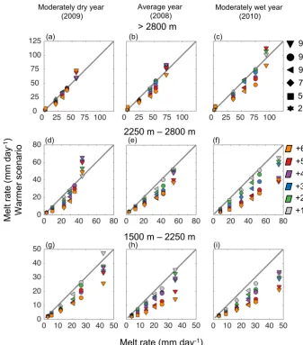
and the year with the most snowfall (and latest storm events) prone to the greatest reductions (Fig. 9). There are notable exceptions. For a majority of the simulations, extreme melt rates (99th percentiles; downward-facing triangles in Fig. 9) actually increase (inferred from markers plotting above the 1:1 line) at elevations > 2800 m a.s.l. in all years (top pan-els) and in the drier year at elevations > 2250 m a.s.l. To better understand why these extreme melt rates differ in trend from the lower percentiles, we provide a brief analysis of 2009 ex-treme melt events. The analysis is limited to elevations above
Nom. +1° C +2° C +3° C +4° C +5° C +6° C Scenario 0.4 0.5 0.6 0.7 0.8 0.9 1
Fraction of historical
total meltwater
Mod. wet year Average year Mod. dry year
y = -0.093x + 1.113
y = -0.105x + 1.099
y = -0.108x + 1.121
Figure 7.The fraction of simulated domain-wide historical meltwa-ter (yaxis), relative to the nominal case, for each warmer temper-ature scenario (xaxis) for the three years (marker type and color). The colored lines and associated regression equations show linear fits to the data. For each year, theR2value was > 0.99 and thep value was1×10−6.
2250 m a.s.l. where a threshold of 40 mm day−1 designates extreme (99th percentiles) melt rates (see Fig. 9).
In the spring, extreme melt affected a very limited portion of the domain on any given day (inferred from blue colors on the right in the top panel of Fig. 10), and the spatial extent of extreme melt generally decreased in response to warm-ing. Conversely, three distinct extreme melt events on 21 Jan-uary, 22 FebrJan-uary, and 1 March 2009 (arrows in Fig. 10) ex-hibit large increases in the fraction of the domain affected, with the January and March events increasing in spatial ex-tent until+4◦C before decreasing with additional warming. The simulated melt events were not associated with sub-stantial rainfall, but rather cloudy and/or windy conditions with high longwave radiation that generally occurred under warmer-than-average temperatures in the nominal case. Mea-sured meteorological conditions for these days are provided in Table 3. These warm and cloudy winter conditions were insufficient to produce widespread extreme melt in the nom-inal case; melt was limited to elevations < 2000 m a.s.l. and generally did not exceed the 99th percentile (Table 3). Ad-ditional warming caused extreme rates of melt to occur at increasingly higher elevations at a time of substantial snow cover (Fig. 10).
4 Discussion
4.1 Snowmelt response to simulated warming
0 500 1000 1500 2000 500
1500 2500 3500
+6 C +4 C +2 C nom.
0 0.2 0.4 0.6 0.8 1 500
1500 2500 3500
0 0.2 0.4 0.6 0.8 1 0 0.2 0.4 0.6 0.8 1 0 500 1000 1500 2000 0 500 1000 1500 2000
-30 30 500 1500 2500 3500
-30 30 -30 30 -30 30 -30 30 -30 30 -30 30 -30 30 -30 30 0 500 1000 1500 2000
500 1500 2500 3500
+6 C +4 C +2 C Nom.
0 0.2 0.4 0.6 0.8 1 500
1500 2500 3500
0 0.2 0.4 0.6 0.8 1 0 0.2 0.4 0.6 0.8 1 0 500 1000 1500 2000 0 500 1000 1500 2000
-30 30 500 1500 2500 3500
-30 30 -30 30 -30 30 -30 30 -30 30 -30 30 -30 30 -30 30
Meltwater, mm
El
eva
tion
,
m
El
eva
tion
,
m
El
eva
tion
,
m
Fraction of meltwater ≥15 mm day-1
Difference relative to nominal case, %
Moderately dry Average Moderately wet
Moderately dry Average Moderately wet
Figure 8. Top row of panels: the elevation distribution (y axes) of the average total depth of annual meltwater (xaxes) simulated for the nominal case (black lines) and select perturbed temperature scenarios (colored lines). Second row of panels: the fraction of annual meltwater produced at snowmelt rates≥15 mm day−1. The colored circles indicate elevations at which simulated melt occurs equally at rates ≥15 mm day−1 and < 15 mm day−1. The lower panels of colored graphs show the differences from the nominal case, reported in percent of annual meltwater, produced at snowmelt rates≥15 mm day−1for the three select scenarios. Results are shown for the moderately dry (2009; left column of plots), near-average (2008; middle column of plots), and moderately wet (2010; right column of plots) snow seasons.
sensitivity. Despite the simplicity of our climate sensitivity method, the predicted sensitivity of total snow volume to warming of −9.3 to −10.8 %◦C−1 is consistent with pre-vious studies using either statistical and dynamical down-scaling of GCM output (Sun et al., 2016;−9.3 %◦C−1)or a simple statistical snow model trained on observations (Howat and Tulaczyk, 2005;−10 %◦C−1). The consistency suggests that these models of varying complexity adequately treat the warming-induced shift from snowfall to rain. This confirms recent findings by Schlögl et al. (2016) that snow model
mag-Melt rate (mm day-1)
Nominal case
Me
lt
ra
te
(mm
da
y
-1)
W
ar
m
er
sce
na
ri
o +6°C
+5°C +4°C +3°C +2°C +1°C Moderately dry year
(2009)
Moderately wet year (2010) Average year
(2008)
1500 m – 2250 m 2250 m – 2800 m
> 2800 m
99th
95th
90th
75th
50th
25th
(a) (b) (c)
(d) (e) (f)
(g) (h) (i)
Figure 9.Quantile plots of simulated melt rates for the nominal (xaxes) and warmer scenarios (yaxes) for model grid cells characterized as high elevation (> 2800 m;a, b, c), middle elevation (2250–2800 m;d, e, f), and lower elevation (1500–2250 m) regions for the moderately dry year(a, d, g), average year(b, e, h), and moderately wet year(c, f, i). Marker colors correspond to the six different temperature perturbations. Plotted in each graph are the 25th, 50th, 75th, 90th, 95th, and 99th percentiles (marker shapes) of daily snowmelt rates≥1 mm day−1for all grid cells within each water year and elevation range. The 1:1 lines are plotted for reference.
nitude (±20 %) did not affect the relative snowpack climate sensitivity to warming. Thus, snowmelt rates may be more sensitive to changes in the seasonal timing of precipitation than to changes in precipitation magnitude. This supports the conclusions of Cooper et al. (2016) that record low snowpack years may not serve as appropriate analogues for the climate sensitivity of snow.
In a warmer climate, shifts from snowfall to rain are likely to combine with shifts in snowmelt timing to cause earlier water availability relative to the historical period. As a re-sult, the ephemeral snow zone is expected to progress up-ward in elevation (Minder, 2010) and shift the areal distribu-tion of SWE toward higher, unmonitored elevadistribu-tions. Indeed, the+3◦C scenario shifted the elevation of maximum annual meltwater volume above that of the highest regional SWE
fS
C
A
F
ra
ct
io
n
o
f d
o
m
a
in
S
ce
n
a
rio
S
ce
n
a
rio
2009
(a)
(b)
Figure 10.Daily extreme snowmelt in 2009 (melt rates > 40 mm day−1at model grid cells > 2250 m a.s.l., corresponding to extreme melt rates,≥99th percentile; see Fig. 8) as simulated by the nominal (Nom.) and six perturbed temperature scenarios (yaxes) shown as the(a)
fraction of the area undergoing extreme melt. The lower panel shows the fraction of snow-covered area (fSCA) for the same time period and domain. Arrows indicate (winter) melt events (see Table 3 for meteorological conditions and averages).
Table 3.Mean daily values of hourly measured meteorological vari-ables (nominal mean) during the three mid-winter melt events in 2009 (see Fig. 10) compared to the average conditions measured at eight stations > 2250 m a.s.l. computed on 11 days centered on the event dates, averaged over the three years of the study. Precipitation is reported as the daily sum of measured values. Melt rates simu-lated in the nominal case are reported as the mean value computed over all grid elements > 2250 m a.s.l. and the maximum value over the full domain with the corresponding elevation.
Met. variable 21 Jan 22 Feb 1 Mar
Air temp.,◦C 2.8/−0.5 −0.7/0.6 4.4/1.0 Shortwave, W m−2 57/96 83/152 163/176 Longwave, W m−2 292/232 297/226 266/217 Wind, m s−1 4.0/4.3 4.6/4.0 7.2/4.4 Precipitation, mm 0.0 4.3 0.0 Mean melt rate, mm d−1 6.5 1.5 4.7 nom. sim. (> 2250 m)
Max. melt rate, mm d−1 30.6 (1897) 28.3 (1586) 44.0 (1741) nom. sim. (elev., m)
elevations, and in wetter, compared to drier snow seasons, is an important factor in interpreting snowmelt temperature sensitivity results.
We show a general tendency toward lower melt rates in re-sponse to warming. In contrast to Musselman et al. (2017), which evaluated mean snowmelt response to a single green-house gas emissions scenario at 4 km resolution, we evaluate a range of potential warming, examine the percentile distri-bution of snowmelt response, and elucidate the process along elevational gradients most relevant to basin-wide runoff. This is a critical advancement in understanding how and where
meltwater production is impacted by warming, an evaluation that cannot be achieved with the type of “high-resolution” climate modeling used in Musselman et al. (2017). Impor-tantly, we report an emergence (i.e., not present in the his-torical simulations) and spatial expansion of extreme winter melt events and, conversely, a decline in extreme melt dur-ing sprdur-ing. Increases in extreme winter melt occurred under warm and cloudy conditions, and decreases in extreme spring melt were due to reduced snow-cover persistence. This is an important new finding with implications on flood hazard and reservoir management. The general tendency toward slower snowmelt rates and higher extreme values is analogous to the expected climate change impacts on precipitation, where high-intensity events are expected to increase despite pro-jected declines in total (e.g., summer) precipitation (Prein et al., 2017; Trenberth, 2011).
4.2 Hydrologic implications
lim-ited area (generally < 30 % of land area above 2250 m a.s.l.) at any given time. This is likely due to snowpack cold con-tent and/or cool air temperatures limiting melt at upper eleva-tions and low snow-cover fraction limiting melt at lower ele-vations. Compared to the historical period, warming doubles the basin area that experiences extreme melt, and shifts its oc-currence from spring to winter. The increased spatial extent, intensity, and frequency of extreme winter snowmelt events may have significant implications for antecedent moisture conditions and associated flood risk.
Snowmelt rates have been mechanistically linked to streamflow production (Barnhart et al., 2016), but less un-derstood are the potential implications of climate-induced changes in snowmelt rates on subsurface water storage, evap-otranspiration, and streamflow response. For example, recent empirical evidence that a precipitation shift from snow to-wards rain will lead to a decrease in streamflow (Berghuijs et al., 2014) lacks definitive causation. Compared to soil, snow cover exhibits different water routing mechanisms. For example, lateral downslope flow of water along snowpack layers has been shown to explain the observed rapid deliv-ery of water to streams and anomalously high contributions of event water to the hydrograph during rain on snow and snowmelt (Eiriksson et al., 2013). One hypothesis is that as snow cover becomes less persistent in a warmer world, and snowmelt rates decline, this rapid slope-scale redistribution of water toward stream channels will slow or cease, increas-ing the soil residence time of water. Longer soil residence time can increase the partitioning of water to evapotranspi-ration, and thus decrease streamflow. While not available in this region, snowmelt lysimeters may be useful additions to long-term research sites to better characterize variability and trends in the flux of water to the soil system.
Other empirical and modeling studies have reported de-clines in summertime streamflow due to earlier snowmelt runoff and earlier depletion of shallow aquifers (Hunting-ton and Niswonger, 2012; Luce and Holden, 2009). Catch-ment wetness (i.e., soil moisture content and shallow ground-water levels) has substantial impact on runoff response in mountainous areas with distinct thresholds determining re-lationships amongst wetness, streamflow, and contributing area (Penna et al., 2011), with behavior controlled by soil type, subsurface storage capacity, and climate. These factors are also important drivers of evapotranspiration (Christensen et al., 2008; Lundquist and Loheide, 2011) and the regional variability of hydrologic sensitivity to climate change (Tague et al., 2008). In this regard, percentage reductions in future streamflow may be more substantial than the meltwater re-ductions reported here because slower snowmelt is less effi-cient at generating streamflow.
4.3 Sources of uncertainty and caveats
Improved model error characterization for the baseline (nom-inal) years is a critical step toward informed interpretation of
the results of our climate change sensitivity analysis. While snow model errors may be less important when relative cli-mate sensitivity metrics are evaluated (Schlögl et al., 2016), runoff simulations require accurate representation of snow-pack volume and melt rates. Simulated snow depth values were within the range of observations from automated sen-sors at four sites spanning elevation, forest density, slope and aspect. This verification provides confidence in the model to capture accumulation, melt rates, and the date of snow disap-pearance across spatial and temporal scales.
Notwithstanding the abovementioned, there are inherent strengths and weaknesses of the different validation data sets. For example, automated SWE stations were often co-located with meteorological stations used to force the model; thus, the full potential for model error may not be evalu-ated at these locations. A fairer model assessment is pos-sible when using data from the plot- and basin-scale snow surveys, which can be farther away from the local meteo-rological stations. In another example, the plot-scale survey design samples many SWE measurements within a 100 m grid cell, while the basin-scale surveys sampled snow depth at only three measurement points, relying on extrapolation from a few density measurements to estimate SWE. The au-tomated SWE stations only sample a single point. The degree to which these point samples represent the average value over an area consistent with the model grid scale is a source of in-herent discrepancy between models and observations, inde-pendent of model skill (Trujillo and Lehning, 2015). Over-all, the model performed best in regions closest to precipi-tation gauges used to force the model (Fig. S1) and tended to slightly overestimate SWE at upper elevations (Table S3) where no precipitation measurements are available. The re-sults complement our finding that the current precipitation and snowpack observation network may be insufficient in a warmer world where the majority of snow water resources shift to higher, unmonitored elevations where snow model error is greatest.
Min-der, 2015; Pepin and Lundquist, 2008), it is possible that we underestimate regional air temperature changes toward the end of the melt season in the warmer scenarios. Such nega-tive temperature biases would cause underestimation of the snow depletion rate and, ultimately, the snowpack sensitivity to warming. However, these biases may be partially mitigated by our assumption that the winter and spring, and nighttime and daytime, air temperatures warm uniformly.
Sublimation estimates of 5 to 9 % in the nominal case to 8 to 14 % in the+6◦C scenario (Table S4) are on the lower-to-middle end of the reported regional values of 2 to 3 % (West and Knoerr, 1959) to 20 % (Marks and Dozier, 1992). The large range highlights challenges and disparities in mea-suring (e.g., Molotch et al., 2007; Sexstone et al., 2016) and modeling (Etchevers et al., 2004) turbulent exchange, which are further compounded in mountainous terrain due to the challenges of wind-flow simulation (Musselman et al., 2015). The simulated reductions in snowmelt volume due to increased sublimation are very small compared to reduc-tions caused by the warming induced shift from snow to rain. However, by not considering blowing snow and subsequent sublimation losses (i.e., overestimating alpine snowpack), we may further underestimate snowpack sensitivity to warming. In light of the potential errors discussed above, our results should be considered somewhat conservative. Longer-term snow and runoff simulations at scales sufficient to resolve mountain climate elevation gradients are needed both as analysis to understand historical conditions (e.g., snow re-analysis by Margulis et al., 2016) and forced by large suites of future climate scenarios (e.g., Eyring et al., 2016) that dy-namically resolve different model realizations of climate re-sponse to different greenhouse gas emissions scenarios. Such efforts will best inform, and constrain the uncertainty of, potential impacts of climate change on flood risk and wa-ter availability. Toward this goal, our work makes inroads to quantify how snowpack and melt dynamics respond to incre-mental warming over an elevation profile characteristic of a foothills-to-headwaters mountain front. The results offer in-sight into the sensitivity of snow water resources to climate change in the Sierra Nevada, California, with implications for other regions as well.
5 Conclusions
We present a climate sensitivity experiment to investigate how historical snow water resources and melt rates respond to successively warmer temperatures over a large elevation gradient in the southern Sierra Nevada, California. Good agreement between simulations and an unprecedented array of ground-based observations of SWE (RMSE≤100 mm; bias better than ±85 mm) and snow depth (within multi-sensor range) is shown. Three primary findings emerge from the simulations. First, the sensitivity of total snow–water vol-ume to warming is−9.3 to−10.8 % per◦C. The snow
sea-son characterized by above-average snowfall and cold spring storm events was most resilient to warming; however, it also exhibited the greatest shift toward slower melt. Thus, snowmelt rates may be more sensitive to changes in the sea-sonal timing of precipitation than to changes in precipitation magnitude. Second, the middle elevations, which are domi-nated by forest cover and comprise a disproportionately large basin area, exhibit the greatest snowpack reductions and the largest shift toward slower snowmelt. Hence, warming-related impacts on runoff production and ecosystem function may be particularly acute in these areas. Third, increases in the frequency, intensity, and spatial extent of extreme win-ter melt events occur with successive warming. Warming-induced extreme (winter) melt impacts an area nearly twice as large as that simulated at any time in the historical period. The changes in extreme snowmelt events have implications for antecedent moisture conditions and associated flood risk. When considered together, the elevation-dependent climate sensitivity of snowmelt revealed herein has broad implica-tions for water supply monitoring, streamflow production, flood control, and ecosystem function in a warmer world.
Data availability. All data and model output presented herein are available upon request from the corresponding author.
The Supplement related to this article is available online at https://doi.org/10.5194/tc-11-2847-2017-supplement.
Competing interests. The authors declare that they have no conflict of interest.
Matt Cooper.
Edited by: Ross Brown
Reviewed by: Brian Henn and Eric Sproles
References
Bales, R. C., Molotch, N. P., Painter, T. H., Dettinger, M. D., Rice, R., and Dozier, J.: Mountain hydrology of the western United States, Water Resour. Res., 42, W08432, https://doi.org/10.1029/2005WR004387, 2006.
Barnett, T. P. and Pierce, D. W.: Sustainable water deliveries from the Colorado River in a changing climate, P. Natl. Acad. Sci., 106, 7334–7338, 2009.
Barnett, T. P., Adam, J. C., and Lettenmaier, D. P.: Potential impacts of a warming climate on water availability in snow-dominated regions, Nature, 438, 303–309, 2005.
Barnhart, T. B., Molotch, N. P., Livneh, B., Harpold, A. A., Knowles, J. F., and Schneider, D.: Snowmelt rate dictates stream-flow, Geophys. Res. Lett., 43, 8006–8016, 2016.
Bartelt, P. and Lehning, M.: A physical SNOWPACK model for the Swiss avalanche warning: Part I: numerical model, Cold Reg. Sci. Technol., 35, 123–145, 2002.
Bavay, M. and Egger, T.: MeteoIO 2.4.2: a preprocessing library for meteorological data, Geosci. Model Dev., 7, 3135–3151, https://doi.org/10.5194/gmd-7-3135-2014, 2014.
Bavay, M., Lehning, M., Jonas, T., and Löwe, H.: Simulations of fu-ture snow cover and discharge in Alpine headwater catchments, Hydrol. Process., 23, 95–108, 2009.
Bavay, M., Grünewald, T., and Lehning, M.: Response of snow cover and runoff to climate change in high Alpine catchments of Eastern Switzerland, Adv. Water Res., 55, 4–16, 2013. Berghuijs, W., Woods, R., and Hrachowitz, M.: A precipitation shift
from snow towards rain leads to a decrease in streamflow, Nat. Clim. Change, 4, 583–586, 2014.
Brown, R. D. and Mote, P. W.: The response of northern hemisphere snow cover to a changing climate*, J. Climate, 22, 2124–2145, 2009.
Cayan, D. R., Maurer, E. P., Dettinger, M. D., Tyree, M., and Hay-hoe, K.: Climate change scenarios for the California region, Cli-matic change, 87, 21–42, 2008.
Christensen, L., Tague, C. L., and Baron, J. S.:, Spatial patterns of simulated transpiration response to climate variability in a snow dominated mountain ecosystem, Hydrol. Process., 22, 3576– 3588, 2008.
Cooper, M. G., Nolin, A. W., and Safeeq, M.:Testing the re-cent snow drought as an analog for climate warming sensitiv-ity of Cascades snowpacks, Environ. Res. Lett., 11, 084009, https://doi.org/10.1088/1748-9326/11/8/084009, 2016.
Dettinger, M.: Climate Change, Atmospheric Rivers, and Floods in California – A Multimodel Analysis of Storm Frequency and Magnitude Changes, J. Am. Water Resour. As., 47, 514–523, 2011.
Dettinger, M. D. and Cayan, D. R.: Large-scale atmospheric forcing of recent trends toward early snowmelt runoff in California, J. Climate, 8, 606–623, 1995.
Dettinger, M. D., Cayan, D. R., Meyer, M. K., and Jeton, A. E.: Sim-ulated hydrologic responses to climate variations and change in
the Merced, Carson, and American River basins, Sierra Nevada, California, 1900–2099, Clim. Change, 62, 283–317, 2004. Eiriksson, D., Whitson, M., Luce, C. H., Marshall, H. P., Bradford,
J., Benner, S. G., Black, T., Hetrick, H., and McNamara, J. P.:An evaluation of the hydrologic relevance of lateral flow in snow at hillslope and catchment scales, Hydrol. Process., 27, 640–654, 2013.
Elder, K., Dozier, J., and Michaelsen, J.: Spatial and temporal varia-tion of net snow accumulavaria-tion in a small alpine watershed, Emer-ald Lake basin, Sierra Nevada, California, USA, Ann. Glaciol., 13, 56–63, 1988.
Etchevers, P., Martin, E., Brown, R., Fierz, C., Lejeune, Y., Bazile, E., Boone, A., Dai, Y.-J., Essery, R., and Fernandez, A.: Vali-dation of the energy budget of an alpine snowpack simulated by several snow models (SnowMIP project), Ann. Glaciol., 38, 150– 158, 2004.
Eyring, V., Bony, S., Meehl, G. A., Senior, C. A., Stevens, B., Stouffer, R. J., and Taylor, K. E.: Overview of the Coupled Model Intercomparison Project Phase 6 (CMIP6) experimen-tal design and organization, Geosci. Model Dev., 9, 1937–1958, https://doi.org/10.5194/gmd-9-1937-2016, 2016.
Flerchinger, G., Xaio, W., Marks, D., Sauer, T., and Yu, Q.: Comparison of algorithms for incoming atmospheric long wave radiation, Water Resour. Res., 45, W03423, https://doi.org/10.1029/2008WR007394, 2009.
Fry, J. A., Xian, G., Jin, S., Dewitz, J. A., Homer, C. G., Limin, Y., Barnes, C. A., Herold, N. D., and Wickham, J. D.: Completion of the 2006 national land cover database for the conterminous United States, Photogr. Eng. Remote Sens., 77, 858–864, 2011. Fyfe, J. C., Derksen, C., Mudryk, L., Flato, G. M., Santer,
B. D., Swart, N. C., Molotch, N. P., Zhang, X., Wan, H., and Arora, V. K.: Large near-term projected snowpack loss over the western United States, Nature Commun., 8, 14996, https://doi.org/10.1038/ncomms14996, 2017.
Girotto, M., Margulis, S. A., and Durand, M.: Probabilistic SWE re-analysis as a generalization of deterministic SWE reconstruction techniques, Hydrol. Process., 28, 3875–3895, 2014a.
Girotto, M., Cortés, G., Margulis, S. A., and Durand, M.: Exam-ining spatial and temporal variability in snow water equivalent using a 27 year reanalysis: Kern River watershed, Sierra Nevada, Water Resour. Res., 50, 6713–6734, 2014b.
Gleason, K. E., Nolin, A. W., and Roth, T. R.: Developing a representative snow-monitoring network in a forested moun-tain watershed, Hydrol. Earth Syst. Sci., 21, 1137–1147, https://doi.org/10.5194/hess-21-1137-2017, 2017.
Gleick, P. H.: The development and testing of a water balance model for climate impact assessment: modeling the Sacramento basin, Water Resour. Res., 23, 1049–1061, 1987.
Gleick, P. H. and Chalecki, E. L.: The impacts of climate changes for water resources of the Colorado and Sacramento-San Joaquin River basins, J. Am. Water Resour. As., 35, 1429–1441, 1999. Godsey, S., Kirchner, J., and Tague, C.: Effects of changes in
winter snowpacks on summer low flows: case studies in the Sierra Nevada, California, USA, Hydrol. Process., 28, 5048– 5064, 2013.
Howat, I. M. and Tulaczyk, S.: Climate sensitivity of spring snow-pack in the Sierra Nevada, J. Geophys. Res.-Earth Surface, 110, https://doi.org/10.1029/2005JF000356, 2005.
Hunsaker, C. T., Whitaker, T. W., and Bales, R. C.: Snowmelt runoff and water yield along elevation and temperature gradients in Cal-ifornia’s Southern Sierra Nevada1, edited, Wiley Online Library, 2012.
Huntington, J. L. and Niswonger, R. G.: Role of surface water and groundwater interactions on projected summertime streamflow in snow dominated regions: An integrated modeling approach, Water Resour. Res., 48, https://doi.org/10.1029/2012WR012319, 2012.
Jepsen, S. M., Molotch, N. P., Williams, M. W., Rittger, K. E., and Sickman, J. O.: Interannual variability of snowmelt in the Sierra Nevada and Rocky Mountains, United States: Ex-amples from two alpine watersheds, Water Resour. Res., 48, https://doi.org/10.1029/2011WR011006, 2012.
Klein Tank, A., Zwiers, F. W., and Zhang, X.: Guidelines on anal-ysis of extremes in a changing climate in support of informed decisions for adaptation, C. D. a. Monitoring, p. 56, World Me-teorological Organization, 2009.
Knowles, N. and Cayan, D. R.: Potential effects of global warming on the Sacramento/San Joaquin watershed and the San Francisco estuary, Geophys. Res. Lett., 29, 38-31–38-34, 2002.
Knowles, N. and Cayan, D. R.: Elevational dependence of projected hydrologic changes in the San Francisco estuary and watershed, Clim. Change, 62, 319–336, 2004.
Knowles, N., Dettinger, M. D., and Cayan, D. R.: Trends in Snow-fall versus RainSnow-fall in the Western United States, J. Climate, 19, 4545–4559, 2006.
Kobierska, F., Jonas, T., Magnusson, J., Zappa, M., Bavay, M., Bosshard„ T., Paul, F., and Bernasconi, S. M.: Climate change effects on snow melt and discharge of a partly glacierized wa-tershed in Central Switzerland (SoilTrec Critical Zone Observa-tory), Appl. Geochem., 26, Supplement, S60–S62, 2011. Kobierska, F., Jonas, T., Zappa, M., Bavay, M., Magnusson, J., and
Bernasconi, S. M.: Future runoff from a partly glacierized water-shed in Central Switzerland: a two-model approach, Adv. Water Res., 55, 204–214, 2013.
Lehning, M., Völksch, I., Gustafsson, D., Nguyen, T. A., Stähli, M., and Zappa, M.: ALPINE3D: a detailed model of mountain surface processes and its application to snow hydrology, Hydrol. Process., 20, 2111–2128, 2006.
Letcher, T. W. and Minder, J. R.: Characterization of the Simu-lated Regional Snow Albedo Feedback Using a Regional Climate Model over Complex Terrain, J. Climate, 28, 7576–7595, 2015. Lettenmaier, D. P. and Gan, T. Y.: Hydrologic sensitivities of the
Sacramento San Joaquin River Basin, California, to global warm-ing, Water Resour. Res., 26, 69–86, 1990.
Lettenmaier, D. P., Wood, A. W., Palmer, R. N., Wood, E. F., and Stakhiv, E. Z.: Water resources implications of global warming: A US regional perspective, Climatic Change, 43, 537–579, 1999. Liston, G. E. and Elder, K.: A Meteorological Distribution System for High-Resolution Terrestrial Modeling (MicroMet), J. Hy-drometeorol., 7, 217–234, 2006.
Liu, C., Ikeda, K., Rasmussen, R., Barlage, M., Newman, A. J., Prein, A. F., Chen, F., Chen, L., Clark, M., and Dai, A.: Continental-scale convection-permitting modeling of the current
and future climate of North America, Clim. Dynam., 49, 71–95, https://doi.org/10.1007/s00382-016-3327-9, 2017.
López-Moreno, J. I., Fassnacht, S., Heath, J., Musselman, K., Re-vuelto, J., Latron, J., Morán-Tejeda, E., and Jonas, T.: Small scale spatial variability of snow density and depth over complex alpine terrain: Implications for estimating snow water equivalent, Adv. Water Res., 55, 40–52, 2013.
López-Moreno, J. I., Mott, R., Faure, F., Lehning, M., Löwe, H., Hynek, B., Michlmayer, G., Prokop, A., and Schöner, W.: Dif-ferent sensitivities of snowpacks to warming in Mediterranean climate mountain areas, Environ. Res. Lett., 49, 155–160, 2017. Luce, C. H. and Holden, Z. A.: Declining annual streamflow dis-tributions in the Pacific Northwest United States, 1948–2006, Geophys. Res. Lett., 36, https://doi.org/10.1029/2009GL039407, 2009.
Lundquist, J. D. and Loheide, S. P.: How evaporative water losses vary between wet and dry water years as a function of elevation in the Sierra Nevada, California, and critical factors for modeling, Water Resour. Res., 47, https://doi.org/10.1029/2010WR010050, 2011.
Magnusson, J., Farinotti, D., Jonas, T., and Bavay, M.: Quantitative evaluation of different hydrological modelling approaches in a partly glacierized Swiss watershed, Hydrol. Process., 25, 2071– 2084, 2011.
Margulis, S. A., Cortés, G., Girotto, M., and Durand, M.: A Landsat-Era Sierra Nevada Snow Reanalysis (1985–2015), J. Hydrometeorol., 17, 1203–1221, 2016.
Marks, D. and Dozier, J.: Climate and energy exchange at the snow surface in the alpine region of the Sierra Nevada: 2. Snow cover energy balance, Water Resour. Res., 28, 3043–3054, 1992. Marks, D., Dozier, J., and Davis, R. E.: Climate and energy
ex-change at the snow surface in the Alpine Region of the Sierra Nevada: 1. Meteorological measurements and monitoring, Water Resour. Res., 28, 3029–3042, 1992.
Marty, C., Schlögl, S., Bavay, M., and Lehning, M.: How much can we save? Impact of different emission scenarios on fu-ture snow cover in the Alps, The Cryosphere, 11, 517–529, https://doi.org/10.5194/tc-11-517-2017, 2017.
McCabe, G. J. and Clark, M. P.: Trends and variability in snowmelt runoff in the western United States, J. Hydrometeorol., 6, 476– 482, 2005.
Michlmayr, G., Lehning, M., Koboltschnig, G., Holzmann, H., Zappa, M., Mott, R., and Schöner, W.: Application of the Alpine 3D model for glacier mass balance and glacier runoff studies at Goldbergkees, Austria, Hydrol. Process., 22, 3941–3949, 2008. Minder, J. R.: The Sensitivity of Mountain Snowpack Accumulation
to Climate Warming, J. Climate, 23, 2634–2650, 2010.
Molotch, N., Colee, M., Bales, R., and Dozier, J.: Estimating the spatial distribution of snow water equivalent in an alpine basin using binary regression tree models: the impact of digital eleva-tion data and independent variable seleceleva-tion, Hydrol. Process., 19, 1459–1479, 2005.
Molotch, N. P. and Meromy, L.: Physiographic and climatic con-trols on snow cover persistence in the Sierra Nevada Mountains, Hydrol. Process., 28, 4573–4586, 2014.