www.the-cryosphere.net/8/345/2014/ doi:10.5194/tc-8-345-2014
© Author(s) 2014. CC Attribution 3.0 License.
The Cryosphere
A range correction for ICESat and its potential impact on ice-sheet
mass balance studies
A. A. Borsa1, G. Moholdt1, H. A. Fricker1, and K. M. Brunt2,3 1Scripps Institution of Oceanography, San Diego, California, USA 2Morgan State University, Baltimore, Maryland, USA
3GESTAR, NASA Goddard Space Flight Center, Greenbelt, Maryland, USA
Correspondence to: A. A. Borsa ([email protected])
Received: 25 July 2013 – Published in The Cryosphere Discuss.: 30 August 2013 Revised: 16 January 2014 – Accepted: 16 January 2014 – Published: 3 March 2014
Abstract. We report on a previously undocumented range er-ror in NASA’s Ice, Cloud and land Elevation Satellite (ICE-Sat) that degrades elevation precision and introduces a small but significant elevation trend over the ICESat mission pe-riod. This range error (the Gaussian-Centroid or “G-C” off-set) varies on a shot-to-shot basis and exhibits increasing scatter when laser transmit energies fall below 20 mJ. Al-though the G-C offset is uncorrelated over periods≤1 day, it evolves over the life of each of ICESat’s three lasers in a series of ramps and jumps that give rise to spurious ele-vation trends of−0.92 to−1.90 cm yr−1, depending on the time period considered. Using ICESat data over the Ross and Filchner–Ronne ice shelves we show that (1) the G-C offset introduces significant biases in ice-shelf mass balance esti-mates, and (2) the mass balance bias can vary between re-gions because of different temporal samplings of ICESat. We can reproduce the effect of the G-C offset over these two ice shelves by fitting trends to sample-weighted mean G-C off-sets for each campaign, suggesting that it may not be nec-essary to fully repeat earlier ICESat studies to determine the impact of the G-C offset on ice-sheet mass balance estimates.
1 Introduction
NASA’s Ice, Cloud, and land Elevation Satellite (ICESat) (Schutz et al., 2005) was an Earth-orbiting laser altimeter mission that operated from 2003–2009. ICESat’s primary task was to repeatedly measure surface elevations along fixed ground tracks over Earth’s polar regions to help quantify the contribution of the ice sheets to contemporary sea level
change. Many studies have used ICESat elevation data to estimate volume/mass changes of glaciers (Gardner et al., 2013), ice shelves (Pritchard et al., 2012), and ice sheets (Shepherd et al., 2012), and ICESat data have been com-bined with other measurements to increase the spatiotem-poral coverage and resolution of surface change estimates. These complementary data include airborne laser altime-try from NASA’s Operation IceBridge mission (Koenig et al., 2010; Kwok et al., 2012; Schenk and Csathó, 2012), gravity from the NASA/DLR GRACE mission (Riva et al., 2009), and elevations from ESA’s ERS-1, ERS-2 and Envisat radar altimeters (Zwally et al., 2011; Hurkmans et al., 2012). ICESat will provide benchmark elevations for the planned ICESat-2 mission (Abdalati et al., 2010), which is planned for launch in 2017 and will extend the satellite laser altime-ter record to 17 yr or more.
(Fricker et al., 2005). ICESat post-launch elevation valida-tion included crossover analysis to determine ICESat’s initial precision and accuracy (Shuman et al., 2006; Brenner et al., 2007), followed by long-term elevation comparisons with re-spect to stable and/or independently characterized reference surfaces (Fricker et al., 2005, Urban and Schutz, 2005; Borsa et al., 2007, 2008; Shuman et al., 2009).
Although ICESat was originally intended to be oper-ated continuously throughout its mission (Abshire et al., 2003), concerns about laser reliability after the failure of the first ICESat laser led to it being operated campaign-style, whereby data were acquired in a series of ∼33-day cam-paigns spaced 4–6 months apart (Table 1). The ICESat val-idation effort focused largely on documenting changes in ICESat elevation accuracy from campaign to campaign and between different releases of ICESat data (e.g., Fricker et al., 2005). Despite ongoing refinements in elevation retrieval (reflected in higher product release numbers), multiple stud-ies have documented persistent instrument-related elevation biases between campaigns (Gunter et al., 2009; Riva et al., 2009; Siegfried et al., 2011). More importantly, these “inter-campaign biases” exhibit statistically significant (albeit dif-ferent) trends over the ICESat mission period (Urban et al., 2012). Furthermore, in the absence of a definitive set of in-tercampaign biases, researchers estimating ice volume/mass balance using ICESat data have taken different approaches with respect to intercampaign bias correction, with some making no correction (Pritchard et al., 2009; Gardner et al., 2013) and others applying biases from one of several sources (e.g., Gunter et al., 2009; Riva et al., 2009; Zwally et al., 2011; Shepherd et al., 2012).
This paper describes a previously unrecognized compo-nent of the ICESat intercampaign biases, an inadvertent range error (called the Gaussian-Centroid or “G-C” offset) that was introduced during the processing of Level 1 data. Correcting for this error improves the precision of individual elevation measurements and removes a small but significant anomalous elevation trend from ICESat data. Using global statistics for the GC offset and case studies over the salar de Uyuni in Bolivia and two Antarctic ice shelves, we demon-strate the potential impact that the correction has on ICESat elevation accuracy and ice sheet mass balance estimates.
2 Data and analysis
2.1 ICESat campaigns
Data collection during the ICESat mission took place dur-ing 18 separate campaigns between February 2003 and Oc-tober 2009 (Table 1). In this paper, we refer to these cam-paigns using the standard convention of pairing the number of the operational laser with a letter designating each consec-utive campaign for that laser (e.g., L2a is the first campaign for Laser 2, L3b is the second campaign for Laser 3, etc.).
Laser 1 operated for only 56 days before it failed and was flown only in ICESat’s 8-day exact-repeat calibration orbit. Most published studies use data from L2a onwards (after the spacecraft had transitioned to its 91-day repeat orbit) so we will focus primarily on Lasers 2 and 3. To clarify the time sequence of the laser campaigns, we note that Laser 2 was switched off after L2c and then back on again after Laser 3 failed, which is why campaigns L2d–L2f took place after L3k (the final Laser 3 campaign).
2.2 ICESat data products
ICESat data are publically available from the National Snow and Ice Data Center (NSIDC, http://nsidc.org/data/icesat/ index.html). Most users of ICESat elevation data choose one of several Level 2 data products containing the geolocated positions of individual laser footprints: GLA06 (Global El-evation Data), GLA12 (Antarctic and Greenland Ice Sheet Altimetry data), GLA13 (Sea Ice Altimetry Data), GLA14 (Global Land Surface Altimetry Data), and GLA15 (Ocean Surface Altimetry Data). Different assumptions about sur-face characteristics and the needs of investigators resulted in differentiation between these data products. Relevant to this study, elevations for GLA06, GLA12, GLA13 and GLA15 were calculated assuming laser reflection from smooth sur-faces such as oceans and ice sheets, which generate simple return waveforms that can be represented accurately by a sin-gle Gaussian peak. Elevations for GLA14 were calculated as-suming complex return waveforms that are best summarized by the centroid of the entire waveform, a distinction that will be discussed later.
In our work, we also used the Level 1A GLA01 (Global Altimetry Data) product to access the individual transmit and return waveforms for each laser shot; the Level 1B GLA05 (Global Waveform-based Range Correction Data) product for waveform parameters such as centroid, Gaussian fit, and skewness; and the Level 1B GLA06 product for instrument pointing, laser energy, surface reflectance, and various cor-rections. Although most users need only Level 2 data (pro-cessed geophysical variables) in their work, access to data in Level 1B (processed instrument) and Level 1A (raw in-strument) products allows investigators such as ourselves to contribute to ICESat calibration and validation efforts. 2.3 Elevation validation at the salar de Uyuni
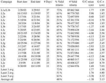
Table 1. ICESat campaign metadata and G-C offset statistics. Campaigns are listed sequentially in time and are named as described in the
text. Laser 2 campaigns are shown in grey to highlight the switching that occurs between lasers during the mission. The valid returns column gives the percentage of shots for which a surface elevation was recorded, which tends to drop as laser energy decreases.
Campaign Start date End date # Days % Valid # Valid G-C mean G-Cσ
returns returns (cm) (cm)
L1a/L1b 2/20/03 3/29/03 37 73 % 85 862 366 1.77 1.99 L2a 10/13/03 11/19/03 37 63 % 80 770 785 5.90 1.83 L2b 2/17/04 3/21/04 33 64 % 72 697 059 0.60 2.07 L2c 5/18/04 6/21/04 34 53 % 62 361 334 −0.16 3.70 L3a 10/3/04 11/8/04 36 64 % 79 437 302 −0.58 1.93 L3b 2/17/05 3/24/05 35 67 % 79 778 747 −1.37 1.95 L3c 5/20/05 6/23/05 34 65 % 75 890 428 −3.44 2.46 L3d 10/21/05 11/24/05 34 63 % 71 662 990 −4.06 2.56 L3e 2/22/06 3/28/06 34 65 % 74 789 938 −4.13 2.10 L3f 5/24/06 6/26/06 33 62 % 71 172 594 −3.72 2.27 L3g 10/25/06 11/27/06 33 61 % 70 179 600 −4.07 2.45 L3h 3/12/07 4/14/07 33 63 % 73 058 093 −3.93 2.23 L3i 10/2/07 11/5/07 34 59 % 68 161 111 −3.86 2.38 L3j 2/17/08 3/21/08 33 63 % 71 872 084 −3.91 2.57 L3k 10/4/08 10/19/08 15 59 % 29 447 798 −4.13 2.66 L2d 11/25/08 12/17/08 22 54 % 40 865 517 −0.11 5.36 L2e 3/9/09 4/11/09 33 39 % 44 606 427 2.65 8.79 L2f 9/30/09 10/11/09 11 35 % 12 844 976 1.69 7.03
Laser 1 avg 73 % 1.77 1.99
Laser 2 avg 51 % 1.76 4.80
Laser 3 avg 63 % −3.38 2.32
Average all 60 % −1.38 3.13
laser footprints from each track fall within the DEM bound-aries. In 2009, we resurveyed the salar de Uyuni to check for topographic change that might impact ICESat elevation validation and found that the DEM – whose error we esti-mate to be less than 2.3 cm root mean square (Borsa et al., 2008) – had risen by an average of 2.5 cm (Brunt et al., 2009). Since we have no information about the nature of the surface change between 2002 and 2009 other than the small change in our DEMs, our best estimate of the actual surface at any intermediate epoch is a linear interpolation between the two DEMs. For the analysis used in this paper, we account for the effect of the surface change by linearly interpolating (node-by-node) between the 2002 and 2009 DEMs to the date of each ICESat pass over the salar, creating a slightly different reference DEM for each track in each campaign.
At the salar de Uyuni, intercampaign biases for the latest release of the ICESat data (R633) ranged over 10 cm, with el-evation biases of up to 17 cm between repeated tracks within a single campaign (see Fricker et al., 2005 for a summary of our methods). These values are of similar magnitude to estimates by other investigators in different locations (Shu-man et al., 2009; Siegfried et al., 2011; Urban et al., 2012). The salar de Uyuni is an ideal validation site – high-elevation (smaller tropospheric delay correction) with negligible cloud cover (little or no multiple scattering) and no topography (lit-tle or no elevation impact from pointing errors) – so we
ex-pected higher accuracy in our elevation recovery than we ob-served. At the same time we realized that with such a large range of observed biases, we had an opportunity to use the salar de Uyuni to search for candidates for the unidentified error sources still affecting ICESat elevations.
2.4 Correlations between transmit pulse parameters and ICESat elevations
For this study, we undertook a systematic examination of the elevation impact of a number of ICESat instrument pa-rameters, motivated by observations made by our group and other investigators that some of these parameters var-ied systematically from campaign to campaign (e.g., Fricker et al., 2005; Shuman et al., 2009). We hypothesized that at the salar de Uyuni we would be able to observe corre-lations between these parameters and the elevation biases still remaining after improvements in ICESat orbit determi-nation, pointing and ranging over the mission lifetime (see http://nsidc.org/data/icesat/past_releases.html). Although we recorded and tracked instrument and environmental informa-tion as part of our validainforma-tion activities, we had not previously looked for quantitative correlations between these parame-ters and the ICESat elevation biases over Uyuni.
-40 -20 0 20 40 relative elevation (cm)
Track 1320
Track 241
Track 360
Track 85 N
10 km
Fig. 1. The reference DEM used in this study, located on the salar de
Uyuni in Bolivia. Topographic relief across the 45-by-54 km DEM is only 80 cm, making this region of the salar one of the flattest natural surfaces on Earth. ICESat tracks 85 (descending) and 360 (ascending) cross the DEM and are used for range validation.
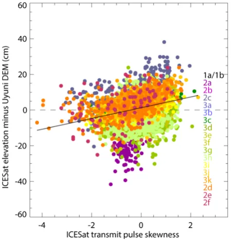
elevations) for all 8371 valid ICESat returns over the salar de Uyuni DEM, without regard to their chronological or-der. We regressed these misfits against a number of instru-ment/waveform parameters and found significant non-zero correlation between the misfits and (1) transmit pulse skew-ness, (2) transmit pulse eccentricity, (3) transmit gain, (4) transmit pulse energy, and (5) receive pulse energy. In the case of transmit pulse skewness, visual examination of the scatterplot between skewness and misfit (Fig. 2a) shows that the two are linearly correlated, with stronger correlations for individual campaigns than for the entire data set. Quantita-tively, the linear Pearson correlation coefficientR between skewness and misfit is 0.30 (and statistically significant) for the entire data set, with values for individual campaigns that reach 0.64 for L2b and L3c. Since parameters 1–2 are re-lated to the transmit pulse shape, and parameters 3–5 are di-rectly or indidi-rectly related to transmit pulse amplitude, we concluded that characteristics of the transmit pulse were af-fecting ICESat range determination and were able to identify a potential mechanism for this effect in the ICESat Range Algorithm Theoretical Basis Document (ATBD) (Brenner et al., 2003).
ICESat’s transmit and return pulses are recorded as his-tograms of energy versus time, with each histogram bin span-ning 1 ns (equivalent to 15 cm in range). Following conven-tion, we refer to these histograms as laser waveforms. ICESat Level 1 data post-processing identifies the times associated with reference points on the transmit and return waveforms and differences the two to obtain the pulse travel time, which is then scaled to obtain the range from ICESat to the surface.
Fig. 2a. Scatterplot of ICESat elevation misfits versus the transmit
pulse skewness for each shot, with the linear correlation between the two indicated by the black line. The Pearson correlation coeffi-cientR is 0.30 for the whole data set, with higher coefficients for most of the individual campaigns – up to 0.64 for L2b and L3c (see campaign color code at right of plot).
Two types of reference point are used in ICESat processing: the centroid of the waveform (yielding timeCTfor the trans-mit waveform or timeCRfor the return waveform) and the
peak position of the Gaussian fit to the waveform (timesGT orGR). For consistency, travel times should be calculated us-ing the same type of reference point on both the transmit and the return waveforms (e.g.,T =CR−CTorT =GR−GT). We noticed, however, that two different reference points were specified in a figure in the ICESat Range ATBD, with the range calculated from the Gaussian-Centroid time difference
GR−CT (see Fig. 3). This is problematic because any dif-ference between the transmit centroid and transmit Gaussian peak location also appears in the return centroid and Gaus-sian. While this has no effect when pulse travel time is calcu-lated between centroids or between Gaussians, when mixed reference points are used it results in a range error that prop-agates through the ICESat geolocation process to yield an elevation error of opposite sign.
2.5 An ICESat range error: the Gaussian-Centroid (G-C) offset
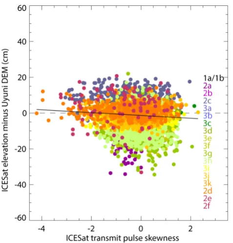
Fig. 2b. Same as Fig. 2a, but using G-C-corrected ICESat
eleva-tions.Ris now only−0.09 for the whole data set, indicating that the G-C correction has removed most of the spurious correlation between transmit pulse skewness and ICESat elevations.
ICESat products except GLA14 (land surface elevations). As discussed earlier, in the case of GLA14 the expectation was that over land the reflecting surface would be complex and the elevation of the laser footprint location would be best summarized by the centroid of the return waveform. GLA14 elevations were therefore implemented using centroid-to-centroid (CR−CT)timing and are not impacted by the G-C offset. For GLA06, GLA12, GLA13, and GLA15, where re-turn waveforms were expected to be primarily single-peaked and Gaussian-shaped, a Gaussian fit was used to determine the time of the return waveform and was (incorrectly) differ-enced with the centroid of the transmit waveform.
Fortunately, the range error in these four data products due to G-C timing (henceforth the “G-C offset”) can be exactly reproduced using the transmit pulse parameters available in the ICESat GLA05 data product:
G−C offset(m)=(GLA05.d_parmTr(2)
−GLA05.d_locTr)·c/2, (1) where d_locTr is the time in ns corresponding to the transmit waveform centroid (parameter names are those used in the GLA05 data product), d_parmTr(2) is the time in ns of the peak of the Gaussian fit to the transmit waveform, andcis the speed of light defined as 0.30 m ns−1. The elevation im-pact of the G-C offset can be removed by adding the offset from (1) directly to ICESat elevations, a step we will refer to as the “G-C correction” hereafter. Alternatively, investigators
GR GT
CT
CR
Return Waveform Range = (GR – CT) *c/2
Transmit Waveform
Return Gaussian Transmit
Gaussian Transmit Pulse
Return Pulse
Fig. 3. ICESat range determination illustration, adapted from
Bren-ner et al. (2003). The transmit and return waveforms are shown in black, and the Gaussian fits to those waveforms are shown in green. The centroids of the transmit (CT)and return (CR)waveforms are indicated by the solid black vertical lines, and the peak locations of the Gaussian fits to the transmit (GT)and return (GR)waveforms are indicated by the dotted green vertical lines. The ICESat range determination algorithm that was implemented through data release R633 used the time difference between the return Gaussian peak and the centroid of the transmit waveform (multiplied by the speed of lightcand divided by 2 to get one-way range), which introduces a range error equal to (GT–CT).
can apply the G-C correction from files provided by the Na-tional Snow and Ice Data Center (http://nsidc.org/data/icesat/ correction-to-product-surface-elevations.html). Technically, the G-C offset/correction should also be scaled by the cosine of the laser pointing angle measured from nadir, but since this angle is rarely over 3◦, the scaling is < 1 mm and is negligible in most cases.
After calculating and applying the G-C correction to ICE-Sat returns from the salar de Uyuni, we revisited our analysis in Sect. 2.4 and confirmed that the G-C offset was responsi-ble for most of the observed correlation between ICESat el-evations and the listed waveform/instrument parameters. As Fig. 2b illustrates for transmit pulse skewness, we observed that correlations drop to nearly zero after the G-C correction is applied to ICESat elevations.
2.6 G-C offset characteristics for ICESat’s three lasers
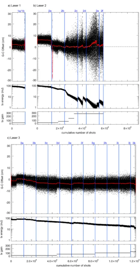
We took the entire ICESat data set and used Eq. (1) to calcu-late the G-C offset for all laser shots that resulted in a valid surface return. Ordering the pulses sequentially by laser shot, we found significant and systematic differences in the G-C offset over the life of each laser and between the three lasers (Fig. 4; Table 1).
Fig. 4. The G-C offset, transmit energy, and transmit gain for Laser
1 (a), Laser 2 (b), and Laser 3 (c), ordered sequentially by the cu-mulative number of shots for each laser. The red line in the top plot is the 10 000-shot moving average of the G-C offset. ICESat cam-paigns are named in blue at the top of the plots and are delineated by blue lines marking the end of each campaign period. The scatter in the G-C offset grows as transmit energy drops, especially below 20 mJ.
low transmit energy because the accompanying decrease in the signal-to-noise ratio of the laser waveforms (once the transmit gain can no longer be increased to compensate) de-grades the precision of centroid determination and Gaussian fitting (Fricker et al., 2005). In addition, there were signif-icant changes in the moving average of the G-C offset (red line in Fig. 4), including (1) a 5 cm drop at the end of L2a that is associated with an instantaneous 10 mJ fall in transmit
Fig. 5. G-C offset campaign means and trend estimates for selected
data spans from Table 2, Trend A. The box symbols indicate the mean values of the G-C offset for each campaign, the error bars show the offset standard deviations, and the different lines are G-C offset trends estimated for different data periods using inverse-variance weighing. The G-C offset has a bigger impact on elevation trends when campaigns at the end of the mission are excluded.
power and is probably due to the failure of one of the diode pump bars, (2) a large negative spike at the beginning of L2b during the period ICESat was in sun acquisition mode, and (3) an inverse correlation with transmit power beginning in L2d, which was when transmit energy fell and remained be-low 10 mJ.
By contrast, Laser 3 showed much more stable G-C off-set behavior, due in part to its higher transmit energies (Fig. 4c). Overall, Laser 3 had a lower mean G-C offset value (−3.38 cm) than the other two lasers and a relatively constant standard deviation (2.32 cm) whose value was close to that of Laser 1. The G-C offset moving average started around 0 cm, jumped 3 cm in the middle of L3a (when the laser tempera-ture was increased from 13.8 to 16.0◦C), and then gradually dropped by 4 cm through L3d and remained consistent up to the end of L3k.
3 Results and discussion
3.1 Trend in the G-C offset over the ICESat mission
There are two direct effects of the G-C offset: (1) it increases the shot-to-shot variability of ICESat elevations (especially at low transmit energies) and (2) it shifts the mean elevation for most campaigns. Of greater relevance to ice-sheet mass balance studies is a secondary effect due to the fact that when ordered in time, the changes in the mean G-C offset between campaigns exhibit time-correlated behavior over the mission period (Fig. 5) that could potentially be interpreted as real surface elevation change. In particular, the high values of the G-C offset for all three campaigns at the end of the mission (L2d–L2f) generate erroneously low elevations that could be interpreted as suddenly higher ice sheet mass-loss rates at the end of the mission period.
Table 2. G-C offset trend estimates (and formal 1-sigma errors) using different data periods and different least-squares weighting applied
to each campaign. Trend A uses inverse-variance weighting derived from the G-C offset statistics in Table 1, Trend B uses uniform weight-ing, and Trend C uses weights derived from global ICESat sampling by campaign. These trend estimates represent the impact of the G-C correction on dh/dt, indicating that all ICESat-derived ice elevation change estimates should become more negative once the G-C offset is removed.
Begin End G-C Trend A G-C Trend B G-C Trend C campaign campaign (cm yr−1) (cm yr−1) (cm yr−1)
L2a L3i −2.13 ±0.53 −1.90 ±0.48 −1.90 ±0.51 L2a L3j −1.88 ±0.47 −1.62 ±0.41 −1.76 ±0.47 L2a L3k −1.64 ±0.41 −1.39 ±0.36 −1.55 ±0.42 L2a L2d −1.54 ±0.40 −1.00 ±0.32 −1.17 ±0.38 L2a L2e −1.48 ±0.40 −0.62 ±0.29 −1.05 ±0.37 L2a L2f −1.38 ±0.40 −0.36 ±0.26 −0.92 ±0.36
area (Schenk and Csathó, 2012 offer an alternative method-ology that accounts for non-linear features in elevation time series). Since we wanted to understand how the G-C offset might have impacted these mass balance estimates, we es-timated the trend of the G-C offset trend over several time periods. First, we performed a linear regression against time of the global mean G-C offsets for campaigns L2a to L2f (the entire mission), with inverse-variance weights for each campaign calculated from the G-C offset standard deviations (all data are from Table 1). This choice of weighting low-ers the contribution of high-variance data points, which in this case are the three Laser 2 campaigns at the end of the mission. For the L2a–L2f period, we obtained a trend of
−1.4±0.4 cm yr−1, which is statistically different from zero at the 3-sigma level. Since many published studies do not in-clude the later ICESat campaigns in their analysis, we also report trends for other data periods (Table 2, Trend A). As Table 2 and Fig. 5 show, the fewer campaigns used at the end of the ICESat mission, the more negative the trend of the G-C offset: up to−2.1±0.5 cm yr−1in the case of data spanning only the period between L2a to L3i.
3.2 Potential impact of the G-C offset on ICESat elevation trends
The negative trend in the G-C offset contributes an erroneous positive trend in ICESat elevations that could be interpreted as real surface change. However, the trends we calculated in Sect. 3.1 are not our best estimate of the actual effect of the G-C offset on ICESat-derived elevation change because of differences in linear regression weighting, as we discuss below.
ICESat investigators typically estimate volume change by integrating many independent elevation trend estimates over a region of interest. If ICESat elevation data are not corrected for the G-C offset, the G-C offsets on all the individual laser shots will propagate through the linear regression used to es-timate elevation trends and will introduce an error. Impor-tantly, this trend error is highly dependent on the weighting
applied to the elevations in the regression (see Appendix A). Since most investigators use constant weighting for all re-turns (e.g., Shepherd et al., 2012), we repeated the linear regressions from Sect. 3.1 using a uniform weight on each campaign of 1/4 cm−2(corresponding to a 2.0 cm standard deviation). The result was less negative G-C offset trends (Table 2, Trend B), with the biggest change for the longest data periods (e.g., for L2a–L2e and L2a–L2f). Using a differ-ent value for the uniform weight will not change these trend estimates, although it will change the formal error.
In addition, the number of ICESat measurements in each campaign (i.e., spatio-temporal sampling) also affects how the G-C offset will affect elevation trend estimates. For ex-ample, campaign L2f had fewer returns than any other cam-paign because it was only 11 days long and because its low laser transmit energy resulted in a low percentage of valid re-turns being recorded due to attenuation by clouds. There are relatively few L2f elevations included in the many thousands of elevation trend estimates made over an ice sheet, which means that campaign L2f elevations (and therefore the G-C offset for L2f) are typically underweighted in the overall ice sheet elevation trend.
3.3 Power spectrum of the G-C offset
To determine if there is regional variation in the G-C off-set, we examined the G-C offset power spectrum to look for temporal correlations that could map into spatial patterns. For this analysis we could not use G-C offsets calculated from the centroid and Gaussian parameters in the GLA05 data product, since shots without a valid return (see Table 1) did not undergo Gaussian fitting during ICESat data process-ing. Spectral estimation requires continuous time series, so we retrieved transmit waveform records from the GLA01 data product, estimated Gaussian fits for every ICESat trans-mit pulse, and recalculated the G-C offset using Eq. (1) and the original GLA05 centroids. The G-C offsets calcu-lated this way deviate from the GLA05-derived offsets by 0.0±2.5 mm (1-sigma) overall and are continuous over each campaign.
We made G-C offset power spectral density (PSD) esti-mates for each of the 18 ICESat campaigns using a single-window Fast Fourier Transform (FFT) with a Hamming ta-per. In all cases, the power spectra are flat at frequencies higher than 10−5Hz, except for narrow spectral peaks at 0.000173 Hz (the orbital frequency of ICESat) and various multiples thereof (Fig. 6). If there were any jumps or ramps in the G-C offset time series during a campaign, these are manifested as a ramp in the spectrum at frequencies lower than 10−5Hz (e.g., Fig. 6, left). What these results indicate is that the G-C offset generally behaves like white noise over periods shorter than a day (about 15 full orbits), with super-imposed sinusoidal variability over distances≤1 orbit. Al-though this implies some degree of along-track correlation, because successive ICESat ground tracks fill in between ear-lier tracks, changes in the G-C offset are almost uniformly distributed over a broad area such as an ice sheet. The global characteristics of the G-C offset should thus be a good first approximation to how it manifests in any regional analysis. 3.4 Impact of the G-C Offset on ICESat dh/dtestimates
over ice shelves
In order to test our assumptions about the impact of the G-C offset on ICESat trend estimates, we did an analysis of data over the Ross and Filchner–Ronne ice shelves in Antarctica. These ice shelves are large, relatively featureless, and are a good analogue for the low-relief interiors of the ice sheets. For each ice shelf we estimated elevation trends for cam-paigns L2a–L2f using ICESat data with and without the G-C offset. For this analysis, we followed the standard approach of simultaneously estimating planar slopes (dh/dx, dh/dy)
and temporal trends (dh/dt )for nearby footprints along seg-ments of ICESat repeat tracks using least-squares estima-tion with unit weighting (e.g., Smith et al., 2009; Gardner et al., 2013). We used saturation-corrected and tide-corrected elevations from the ICESat GLA12 data product, “retided” the elevations using a more accurate tide-model (Padman et
al., 2002; Fricker and Padman, 2006), and estimated dh/dt
only for tracks that were repeated during four or more cam-paigns. Finally, for each ice shelf and data set, we calculated a latitude-weighted average dh/dtvalue by applying an em-pirical function of the satellite orbit convergence towards the geographical poles (Gardner et al., 2013). This provides a weighted estimate of dh/dt that is consistent with gridding methods, although without the need for spatial interpolation. For both ice shelves, the impact of the G-C correction was that the average dh/dt value became more negative, on the order of 0.6 cm yr−1. For the Ross Ice Shelf, the aver-age dh/dt value changed by −0.68 cm yr−1 after applying the G-C correction (from+0.16 cm yr−1to−0.52 cm yr−1). For the Filchner–Ronne Ice Shelf, the average dh/dt value changed by−0.49 cm yr−1after applying the G-C correction (from+1.78 cm yr−1to+1.29 cm yr−1). The reason the im-pact of the G-C correction is different on each ice shelf is because the spatio-temporal sampling in each campaign is different. Most relevant is the undersampling of the Filchner– Ronne Ice Shelf in campaign L2a relative to the Ross Ice Shelf (see Table 3), which slightly flattens the G-C correc-tion trend. This can be understood by observing that reduc-ing the weight of L2a in Fig. 5 will mitigate the impact of its high G-C offset and thus flatten the slope of the linear fit to the G-C offsets. Sampling in campaigns L3g and L3i is also different on the two ice shelves, but these differences matter less because L3g and L3i are close to the center of the time series and because their mean G-C offset values are similar to those of nearby campaigns.
The G-C correction significantly changed the mass bal-ance of the two ice shelves we examined. Because of hy-drostatic equilibrium, a given change in surface elevation equates to about nine times more change in ice thickness, greatly magnifying the mass balance impact of systematic measurement errors. In the case of the Ross Ice Shelf, the
−0.68 cm yr−1 change in average dh/dt from the G-C cor-rection implied a mass balance corcor-rection of−29 Gt yr−1 af-ter accounting for hydrostatic equilibrium. The mass balance correction for the Filchner-Ronne Ice Shelf was 18 Gt yr−1.
For comparison, we also approximated the impact of the G-C correction on the ice shelf elevation trend using linear fits to the mean G-C offsets of each campaign. For each ice shelf, we linearly regressed the mean G-C offsets from Ta-ble 1 against time, using the campaign sampling from TaTa-ble 3 to derive appropriate weights via Eq. (A10) (Appendix A). Our estimates for the impact of the G-C correction using this method were−0.61 cm yr−1for the Ross Ice Shelf and
Table 3. ICESat sampling of the Ross and Filchner–Ronne ice
shelves for the elevation trend estimates in Sect. 3.4. We list the number of shots used by campaign over the entire ice sheet (Si in
Eq. A10), as well as the relative campaign sampling weights (ex-pressed as a percentage of the maximum number of shots on that ice shelf for any campaign). There are large differences in relative campaign sampling between the two ice shelves for L2a, L3g and L3j, which results in different estimates for the elevation trend im-pact of the G-C offset.
Campaign Ross Filchner–Ronne # Shots used % Max # Shots used % Max
L2a 395 218 96 179 955 68
L2b 285 648 69 198 316 75
L2c 378 640 92 244 073 92
L3a 377 854 91 245 864 93
L3b 335 248 81 202 618 77
L3c 363 814 88 264 081 100
L3d 358 902 87 197 763 75
L3e 291 486 71 151 919 58
L3f 368 413 89 234 540 89
L3g 413 425 100 169 199 64
L3h 329 989 80 227 046 86
L3i 384 517 93 235 922 89
L3j 262 832 64 220 324 83
L3k 160 299 39 127 620 48
L2d 189 205 46 123 881 47
L2e 261 577 63 190 585 72
L2f 104 189 25 49 165 19
3.5 Impact of the G-C offset on ICESat intercampaign biases
There have been many independent estimates made of ICE-Sat intercampaign biases (e.g., Siegfried et al., 2011; Zwally et al., 2011; Shepherd et al., 2012; Ewert et al., 2012; Gunter et al., 2013; Hofton et al., 2013), many of which were di-rectly compared in Urban et al. (2012). There is little con-sensus between estimates of individual biases or bias trends: the seven estimates considered in Urban et al. (2012) yielded biases that differed by up to 20 cm for any single campaign and bias trends that ranged from−0.3 to+2.2 cm yr−1over the L2a–L2f period. Given the different surface types, data locations, spatial sampling, and methodologies used in these estimates, it is not surprising that the estimated biases dif-fer. However, since the intercampaign bias trends (or their underlying biases) are supposed to be applied as corrections to all ICESat data, it is important to understand the reasons for and implications of the variability between the different estimates.
We identify three components of the measured intercam-paign biases: (1) the contribution of the G-C offset; (2) bias due to all other instrument error sources; and (3) bias esti-mation errors due to actual elevation/range changes from un-modeled physical processes such as surface change and at-mospheric scattering over the selected calibration surfaces.
The contributions of all three components will vary accord-ing to the data and methodology used in the bias estimation. For instance, we demonstrated in Sect. 3.4 how the impact of the G-C offset differs by a few mm yr−1between two ice shelves on the same continent because of different spatio-temporal data sampling. We might also expect, for example, differences between land-, ocean- and ice-determined biases due to systematic differences in cloud cover or surface ge-ometry (e.g., sea-state effects). Larger differences are likely if biases are being estimated over surfaces that are assumed to be stable but are not, or over surfaces whose time variance is imperfectly known.
Applying the G-C correction removes the first component of the intercampaign biases and thus will alter existing in-tercampaign bias estimates. Specifically, we can expect the G-C correction to decrease intercampaign bias trends by 0.92 to 1.90 cm yr−1depending on the campaigns used (Table 2, Trend C). This means that the G-C offset is a significant contributor to the intercampaign biases, although the large spread of the intercampaign bias estimates suggests that sig-nificant residual variability will remain in all estimates af-ter the G-C correction – at the level of individual campaign biases and/or in the overall trends themselves. Validation using the two ICESat tracks that cross the salar de Uyuni DEM (Fig. 1) confirms that the impact on the fitted eleva-tion trend from applying the G-C correceleva-tion to individual ICESat shots is almost the same as what we predict from the global analysis in Sect. 3.2 (−0.92 cm yr−1predicted vs.
−1.17 cm yr−1actual for L2a–L2f). However, the magnitude of the Uyuni intercampaign bias trend (which changed from 0.67±0.47 cm yr−1to−0.50±0.36 cm yr−1) did not appre-ciably drop, which illustrates our point that post-correction errors are likely to remain despite improvements in accuracy and precision.
Of importance to previous studies that used data contain-ing the G-C offset, recent studies have suggested (e.g., Rig-not et al., 2013) that applying a set of intercampaign biases implicitly corrects for the impact of the G-C offset, at least at the level of the mean elevation for each campaign. While technically true, we are concerned that this is not a satisfac-tory way to make the G-C correction. Applying empirical intercampaign biases may partially correct the effect of the G-C offset, but the variability of intercampaign biases from different sources suggests that this approach can introduce additional errors in dh/dtestimates. We recommend instead that investigators explicitly correct for the known G-C offset using one of the methods described in Sect. 2.4.
Finally, we consider whether intercampaign biases should be applied after making the G-C correction. Investigators should be aware that:
1. There is still no authorized or consensus set of inter-campaign biases.
Fig. 6. Power spectrum of G-C offset for campaigns L3a (left) and L3c (right), showing a flat spectrum beyond 10−5Hz, narrow spectral peaks at harmonics of the orbital frequency of ICESat, and different behavior at lower frequencies. The main difference between the two campaigns is that the moving average of the G-C offset jumps abruptly in L3a while it is flat in L3c (see Fig. 4b).
3. Bias estimates must be G-C-corrected before being ap-plied to G-C-corrected elevations.
4. The biases for each campaign should be applied to in-dividual elevations before dh/dt is estimated. Those who wish to apply intercampaign bias trends directly to dh/dtestimates should be aware that they must cor-rect bias trends for sampling effects and the weights used in the dh/dtcalculation, as discussed earlier.
4 Conclusions and outlook
We have reported on a range correction to the ICESat Level 1 data that removes the effect of an erroneous travel time calculation in the Level 1 data (the G-C offset). The impact of the G-C offset on ice-sheet elevation trends (dh/dt )can vary substantially depending on the time span of investiga-tion and the data sampling in each observainvestiga-tion campaign. If those factors are carefully considered, we have shown that it is possible to reproduce the effect of the G-C off-set to within a few mm yr−1 at a regional scale. Ideally, users should apply the G-C offset corrections to the data themselves based on the GLA05 data product or use cor-rection files provided by NSIDC (http://nsidc.org/data/icesat/ correction-to-product-surface-elevations.html) until a final release of the ICESat data becomes available.
Additional work is still needed to characterize the eleva-tion errors that will remain after the G-C offset is removed. This work includes the revision and ultimate reconciliation of various estimates of ICESat intercampaign biases, which
will change as a result of the G-C offset correction. The large variation in existing estimates of intercampaign biases sug-gests that the problem of estimating empirical errors is not necessarily any easier than uncovering the root sources of those errors. We also wonder if the formalization of the in-tercampaign bias as a description for otherwise unmodeled and persistent errors in ICESat elevations may have diverted attention away from the need for a more systematic and me-thodical effort to identify outstanding error sources in the ICESat data. In particular, we are concerned that a single “universal” set of intercampaign biases (were one to become available) would not be equally relevant across a range of studies using different spatial subsets of data or different data sampling/editing.
Appendix A
Linear regression of mean G-C offsets to estimate the G-C impact on ICESat elevation trends
We take the chi-square merit function for the linear fit toN
pairs of time/elevation data to be
χ2(a, b)=
N−1
X
i=0
(h
i+1hi)−(a+bti)
σi
2
, (A1)
where the ti are points in time corresponding to different
ICESat campaigns,hi are the true surface elevations, 1hi
are the corresponding G-C offsets, andσi are the standard
deviations assumed for (hi+1hi). The maximum likelihood
estimate of the slope (or trend)bof the linear fit is the closed-form solution obtained from minimizing A1 (Press et al., 2007) b= P i 1
σi2
P
i
(hi+1hi)ti
σi2
− P i ti
σi2
P
i hi+1hi
σi2
P
i
1
σi2
P
i ti2 σi2
− P i ti
σi2
2 . (A2)
Since A2 is linear inh+1hi, it can be rewritten as the
sum of separate solutions forhand1hi
b=
P
i
1
σi2
P
i hiti
σi2
− P i ti
σi2
P
i hi
σi2
P
i
1
σi2
P
i t2
i
σi2
− P i ti
σi2
2 + P i 1
σi2
P
i 1hiti
σi2
− P i ti
σi2
P
i 1hi
σi2
P
i
1
σi2
P
i t2
i
σi2
− P i ti
σi2
2 (A3)
or
b=bsurface+bG−C. (A4)
The contribution of the G-C offset to the trend in the data can therefore be considered separately from the contribution of the surface elevations themselves, although the weighting will be the same in both cases.
To scale these conclusions from a single evaluation cell to an entire study area, we note that the ice volume change for a given region is calculated by summing the contribution of many independent trend estimates
dV
dt = X
j
bjAj=
X
j
bsurfacej+bG−Cj
Aj
=X
j
h
bsurfacejAj+bG−CjAj
i
(A5)
with separate terms for the true surface volume change and volume change from the G-C offset. If we make the simplify-ing assumption that the areaAjof each evaluation cell is the
same (most studies interpolate volume/mass estimates to the nodes of a regular grid) and takeMto be the number of cells, the G-C volume change term from Eq. (A5) can be written
dVG−C dt =A
M−1
X
j=0
bG−Cj=MA
M−1
X
j=0
bG−Cj
M . (A6)
Substituting into Eq. (A6) the linear regression solution for
bG−Cfrom Eq. (A3), taking the values forti andσi to be the
same everywhere for a given campaign (although different between campaigns), and distributing the summation overj
gives dVG−C
dt =
MA
P
i
1
σi2
P
i ti
σi21
¯ hi − P i ti
σi2
P
i
1
σi21
¯ hi P i 1 σ2 i P i ti2 σ2 i − P i ti σ2 i 2 (A7) where
1h¯i=
M−1
X
j=0
1hij
M (A8)
is the mean G-C offset value for the campaign indexed byi, and
P
i
1
σi2
P
i ti
σi21
¯ hi − P i ti
σi2
P
i
1
σi21
¯ hi P i 1 σ2 i P i ti2 σ2 i − P i ti σ2 i 2 (A9)
is the maximum likelihood estimate of the G-C offset trend from the mean G-C offsets1h¯i.
Estimates of1h¯i are given in Table 1 (mean G-C offset by
campaign), which our analysis in Sect. 3.3 suggests should be valid anywhere on Earth. Equation (A9) is evaluated by estimating the linear trend1h¯i ordered in time (using
what-everσi were chosen for the surface change analysis) and the
result is used in A7 to estimate the impact of the G-C offset on ICESat elevation change trends assuming identical sam-pling of the various ICESat campaigns.
it is beyond the scope of this paper to offer a proof, boot-strap analysis will confirm that a weighting that accounts for non-uniform sampling is
σi2=σ
2
i
Si
P Si
N , (A10)
where theSiare the number of samples for a given campaign
in the study area andNis the total number of campaigns (as in Eq. A1). This formulation roughly preserves the value of the formal error on the slope estimate obtained from uniform-variance weighting. In the uniform-uniform-variance scenario typical for ICESat, what matters for the trend estimate is the rela-tive number of samples between campaigns, not the absolute numbers.
Acknowledgements. The authors would like to acknowledge the
valuable critique and feedback provided by J. Zwally and his group at NASA’s Goddard Space Flight Center on an earlier version of this manuscript. We would also like to thank M. Siegfried of the Scripps Institution of Oceanography for an early internal review of the manuscript, and B. Csatho and an anonymous reviewer for their helpful review comments. This work was supported by NASA’s Research Opportunities in Space and Earth Sciences program under grant number NNX12AG67G.
Edited by: I. M. Howat
References
Abdalati, W., Zwally, H. J., Bindschadler, R., Csatho, B., Far-rell, S., Fricker, H., Harding, D., Kwok, R., Lefsky, M., Markus, T., Marshak, A., Neumann, T., Palm, S., Schutz, B., Smith, B., Spinhirne, J., and Webb, C.: The ICESat-2 laser altimetry mission, Proceedings of the IEEE, 98, 735–751, doi:10.1109/JPROC.2009.2034765, 2010.
Abshire, J. B., Sun, X., Riris, H., Sirota, M., McGarry, J., Palm, S., Ketchum, E. A., and Follas, R. B.: Geoscience Laser Altime-ter System (GLAS) on the ICESat Mission: Pre-launch and on-orbit measurement performance, Geoscience and Remote Sens-ing Symposium, 2003, ProceedSens-ings, 21–25, July 2003.
Borsa, A. A., Minster, J. B., Bills, B. G., and Fricker, H. A.: Model-ing long-period noise in kinematic GPS applications, J. Geodesy, 81, 157–170, doi:10.1007/s00190-006-0097-x, 2007.
Borsa, A. A., Fricker, H. A., Bills, B. G., Minster, J. B., Caraba-jal, C. C., and Quinn, K. J.: Topography of the salar de Uyuni, Bolivia from kinematic GPS, Geophys. J. Int., 172, 31–40, doi:10.1111/j.1365-246X.2007.03604.x, 2008.
Brenner, A. C., Zwally, H. J., Bentley, C. R., Csathó, B. M., Hard-ing, D. J., Hofton, M. A., Minster, J.-B., Roberts, L. A. Saba, J. L., Thomas, R. H., and Yi, D.: Derivation of range and range distributions from laser pulse waveform analysis for sur-face elevations, roughness, slope, and vegetation heights, Al-gorithm Theoretical Basis Document, version 4.1 (available at: http://www.csr.utexas.edu/glas/atbd.html), Cent. for Space Res., Univ. of Tex., Austin, 2003.
Brenner, A. C., DiMarzio, J., and Zwally, H. J.: Precision and Ac-curacy of Satellite Radar and Laser Altimeter Data Over the
Continental Ice Sheets, IEEE T. Geosci. Remote, 45, 321–331, doi:10.1109/TGRS.2006.887172, 2007.
Brunt, K. M., Borsa, A. A., and Fricker, H. A.: Repeated GPS sur-veys of the salar de Uyuni for continued calibration of ICESat altimeter data, Fall Meeting, AGU, San Francisco, CA, 14–18 December, 2009.
Ewert, H., Popov, S. V., Richter, A., Schwabe, J., Scheinert, M., and Dietrich, R.: Precise analysis of ICESat altimetry data and as-sessment of the hydrostatic equilibrium for subglacial Lake Vos-tok, East Antarctica, Geophys. J. Int., 191, 557–568, 2012. Fricker, H. A., Borsa, A., Minster, B., Carabajal, C., Quinn,
K., and Bill, B.: Assessment of ICESat performance at the salar de Uyuni, Bolivia, Geophys. Res. Lett., 32, L21S06, doi:10.1029/2005GL023423, 2005.
Fricker, H. A. and Padman, L.: Ice shelf grounding zone structure from ICESat laser altimetry, Geophys. Res. Lett., 33, L15502, doi:10.1029/2006GL026907, 2006.
Gardner, A. S., Moholdt, G., Cogley, J. G., Wouters, B., Arendt, A. A., Wahr, J., Berthier, E., Hock, R., Pfeffer, W. T., Kaser, G., Ligtenberg, S. R. M., Bolch, T., Sharp, M. J., Hagen, J. O., van den Broeke, M. R., and Paul, F.: A Reconciled Estimate of Glacier Contributions to Sea Level Rise: 2003 to 2009, Science, 340, 852–857, doi:10.1029/2011GL046583, 2013.
Gunter, B., Urban, T., Riva, R., Helsen, M., Harpold, R., Poole, S., Nagel, P., Schutz, B., and Tapley, B.: A comparison of coincident GRACE and ICESat data over Antarctica, J. Geodesy, 83, 1051– 1060, doi:10.1007/s00190-009-0323-4, 2009.
Gunter, B. C., Didova, O., Riva, R. E. M., Ligtenberg, S. R. M., Lenaerts, J. T. M., King, M. A., van den Broeke, M. R., and Urban, T.: Empirical estimation of present-day Antarctic glacial isostatic adjustment and ice mass change, The Cryosphere Dis-cuss., 7, 3497–3541, doi:10.5194/tcd-7-3497-2013, 2013. Hofton, M. A., Luthcke, S. B., and Blair, J. B.: Estimation of
ICESat intercampaign elevation biases from comparison of li-dar data in East Antarctica, Geophys. Res. Lett., 40, 5689–5703, doi:10.1002/2013GL057652, 2013.
Hurkmans, R. T. W. L., Bamber, J. L., and Griggs, J. A.: Brief com-munication “Importance of slope-induced error correction in vol-ume change estimates from radar altimetry”, The Cryosphere, 6, 447–451, doi:10.5194/tc-6-447-2012, 2012.
Koenig, L., Martin, S., Studinger, M., and Sonntag, J.: Polar Air-borne Observations Fill Gap in Satellite Data, EOS Trans. AGU, 91, 38, 2010.
Kwok, R., Cunningham, G. F., Manizase, S. S., and Krabill, W. B.: Arctic sea ice freeboard from IceBridge acquisitions in 2009: Estimates and comparisons with ICESat, J. Geophys. Res., 117, C02018, doi:10.1029/2011JC007654, 2012.
Luthcke, S. B., Rowlands, D. D., Williams, T. A., and Sirota, M.: Reduction of ICESat systematic geolocation errors and the im-pact on ice sheet elevation change detection, Geophys. Res. Lett., 32, L21S05, doi:10.1029/2005GL023689, 2005.
Magruder, L. A., Webb, C. E., Urban, T. J., Silverberg, E. C., and Schutz, B. E.: ICESat altimetry data product verification at white sands space harbor, IEEE T. Geosci. Remote, 45, 147–155, doi:10.1109/TGRS.2006.885070, 2007.
Padman, L., Fricker, H. A., Coleman R., Howard S. L., and Ero-feeva, S.: A new tide model for the Antarctic ice shelves and seas, Ann. Glaciol., 34, 247–254, 2002.
Press, W. H., Teukolsky, S. A., Vetterling, W. T., and Flannery, B. P.: Numerical Recipes: The Art of Scientific Computing, 3rd Edn., Cambridge University Press, New York, 2007.
Pritchard, H. D., Arthern, R. J., Vaughan, D. G., and Edwards, L. A.: Extensive dynamic thinning on the margins of the Greenland and Antarctic ice sheets, Nature, 461, 971–975, doi:10.1038/nature08471, 2009.
Pritchard, H. D., Ligtenberg, S. R. M., Fricker, H. A., Vaughan, D. G., Van den Broeke, M. R., and Padman, L.: Antarctic ice-sheet loss driven by basal melting of ice shelves, Nature, 484, 502–505, doi:10.1038/nature10968, 2012.
Rignot, E., Jacobs, S., Mouginot, J. and Scheuchl, B.: Ice shelf melting around Antarctic, Science, 341, 266–270, doi:10.1126/science.1235798, 2013.
Riva, R. E. M., Gunter, B. C., Urban, T. J., Vermeersen, B. L. A., Lindenbergh, R. C., Helsen, M. M., Bamber, J. L., van de Wal, R. S. W., van den Broeke, M. R., and Schutz, B. E.: Glacial isostatic adjustment over Antarctica from combined ICESat and GRACE satellite data, Earth Planet. Sc. Lett., 288, 516–523, doi:10.1016/j.epsl.2009.10.013, 2009.
Schenk, T. and Csathó, B.: A New Methodology for Detecting Ice Sheet Surface Elevation Changes From Laser Altimetry Data, Geoscience and Remote Sensing, IEEE T. Geosci. Remote, 50, 3302–3316, doi:10.1109/TGRS.2011.2182357, 2012.
Schutz, B. E., Zwally, H. J., Shuman, C. A., Hancock, D., and Di-Marzio, J. P.: Overview of the ICESat Mission, Geophys. Res. Lett., 32, L21S01, doi:10.1029/2005GL024009, 2005.
Shepherd, A., Ivins, E. R., Geruo, A., Barletta, V. R., Bentley, M. J., Bettadpur, S., Briggs, K. H., Bromwich, D. H., Forsberg, R., Galin, N., Horwath, M., Jacobs, S., Joughin, I., King, M. A., Lenaerts, J. T. M., Li, J., Ligtenberg, S. R. M., Luckman, A., Luthcke, S. B., McMillan, M., Meister, R., Milne, G., Mouginot, J., Muir, A., Nicolas, J. P., Paden, J., Payne, A. J., Pritchard, H., Rignot, E., Rott, H., Sørensen, L. S., Scambos, T. A., Scheuchl, B., Schrama, E. J. O., Smith, B., Sundal, A. V., van Angelen, J. H., van de Berg, W. J., van den Broeke, M. R., Vaughan, D. G., Velicogna, I., Wahr, J., Whitehouse, P. L., Wingham, D. J., Yi, D., Young, D., and Zwally, H. J.: A reconciled esti-mate of ice-sheet mass balance, Science, 338, 6111, 1183–1189, doi:10.1126/science.1228102, 2012.
Siegfried, M. R., Hawley, R. L., and Burkhart, J. F.: High-resolution ground-based GPS measurements show intercampaign bias in ICESat elevation data near Summit, Greenland, IEEE T. Geosci. Remote, 49, 3393–3400, doi:10.1109/TGRS.2011.2127483, 2011.
Shuman, C. A., Zwally, H. J., Schutz, B. E., Brenner, A. C., Di-Marzio, J. P., Suchdeo, V. P., and Fricker, H. A.: ICESat Antarctic elevation data: preliminary precision and accuracy assessment, Geophys. Res. Lett., 33, L07501, doi:10.1029/2005GL025227, 2006.
Shuman, C. A., Harding, D. J., Dimarzio, J. P., Sun, X., Suchdeo, V. P., and Brenner, A.: Empirical correction of residual error in the ICESat-1 altimetry time series at Lake Vostok, Fall Meeting, AGU, San Francisco, CA, 14–18 December, 2009.
Smith, B. E., Fricker, H. A., Joughin, I. R., and Tulaczyk, S.: An inventory of active subglacial lakes in Antarctica detected by ICESat (2003–2008), J. Glaciol., 55, 573–595, doi:10.3189/002214311795306682, 2009.
Urban, T. J. and Schutz, B. E.: ICESat sea level comparisons, Geo-phys. Res. Lett., 32, L23S10, doi:10.1029/2005GL024306, 2005. Urban, T., Borsa, A., Brunt, K., Felikson, D., Fricker, H., Hawley, B., Hofton, M., Luthcke, S., Pie, N., Schutz, B., Shuman, C., Yi, D., and Zwally, J.: Summary of ICESat-1 inter-campaign el-evation biases and detection methods, Fall Meeting, AGU, San Francisco, CA, 3–7 December, 2012.
Zwally, H. J., Schutz, B. E., Abdalati, W., Abshire, J. B., Bentley, C. R., Brenner, A. C., Bufton, J. L., Dezio, J.,Hancock, D., Harding, D. J., Herring, T. A., Minster, J. B., Quinn, K., Palm, S., Spin-hirne, J. D., and Thomas, R. H.: ICESat’s laser measurements of polar ice, atmosphere, ocean and land, J. Geodyn., 34, 405–445, doi:10.1016/S0264-3707(02)00042-X, 2002.