Abstract-- Trajectory planning is the most crucial part in robot design especially for exoskeleton robot. The suitable trajectory will directly affect safety, health, and comfort of the wearer. In trajectory generation profile of lower limb exoskeleton robot, the cubic polynomial is commonly used to generate smooth trajectory generation profile. Whereas, the quintic polynomial is not widely used due to complexity. This paper aims to make comparative studies between cubic and quintic polynomials. Whereas, the accuracy of generated profile will be investigated and analyzed to understand the gap of knowledge. Based on that, the gait cycle motion is divided into seven sub-phases. Each sub-phase is presented by one polynomial equation either cubic or quintic. Accuracy analysis was involved in order to show either cubic or quintic polynomial is accurately matched to human walking motion profile. The result shows that quintic generates an accurate profile motion of ankle, knee, and hip joints with 0.48520,0.42830, 0.39170 RMS error respectively. Meanwhile, cubic polynomial generates the trajectory motion profile of ankle, knee, hip joints with 0.84170, 0.97280, 0.26390 RMS error respectively. Thus, the quintic polynomial is more accurate than cubic polynomial to generate trajectory profile with the smooth transition.
Index Term-- Trajectory Generation, Cubic Polynomial, Quintic Polynomial, Exoskeletons Robot, Gait Cycle Motion.
1. INTRODUCTION
Most of the robots, such as exoskeleton robot, assistant surgical robot, and humanoid robot need a guidance of human. The trajectory of this robot can be categorized into three types: trajectory planning, path planning, and joint angle tracking. The trajectory planning is used to generate the trajectory based on the joint space by setting the desired joint angles. The path planning is used to generate the trajectory by obtaining the initial point to the final point of the path. The joint angle tracking is used to generate the trajectory by using the PD/PID controller in order to make the joints tracking the desired angles that are generated by trajectory planning [1].
Most of the researchers implement task space [2-6]. They need to solve the robot inverse kinematics which requires knowledge of each end effector position and may have an empty solution space. The approximate solution relies on iterative optimization. There are a few researchers that implement joint space to generate trajectories [7, 8].
Whereas the trajectory generation using joint space is associated with time, and the trajectory generation in task space gives space relation [9].
The trajectory generation of the exoskeleton robot can be divided into three levels: off-line, on-line, and combination of off-line and on-line [10].
The trajectory is described as the desired motion of a manipulator in multidimensional space. At the same time, the trajectory can be described in term of position, velocity, and acceleration with considering time for each degree of freedom [11]. Furthermore, More complex trajectories are able to satisfy desired kinematics parameters constraints such as velocity, acceleration and as well as jerk [12]. The trajectory can be generated by one of the trajectory generation methods categories such as polynomial, trigonometric, and exponential or by the combination of them [12].
Polynomial trajectory algorithm based on Hermite Spline interpolation has been used to generate walking trajectories for different topography condition [13]. It is applied to a biped robot of 10 DOFs. Cubic spline and Hermite polynomial interpolation are also used to generate walking trajectory for 8 Degrees of freedom Biped Robot [14].
Third-order spline interpolation based trajectory planning method is used to generate the smooth trajectory of biped swing leg by reducing the impact effect of instant velocity change during the swing leg touch the ground [15].
Other implemented cubic polynomial to generate the trajectory generation either for biped robot or exoskeleton robot [16-18]. However, the limitation of the cubic polynomial can be noticed when generating linear acceleration profile that leads to infinite spikes jerk at initial and final of the gait cycle motion.
The quintic polynomial has been suggested by [17, 19, 20-22] to be able specifying the position, velocity, and acceleration at the started and ended points of each path. It is also used to solve the linearity of the acceleration that occurred in the cubic polynomial. The quintic polynomial has been used for human trajectory generation for lower limb based on sub-phases [23].
In this paper, comparison on the trajectory generation profile using quintic and cubic polynomial was discussed.
Comparative Study Between Quintic and
Cubic Polynomial Equations Based Walking
Trajectory of Exoskeleton System
1
MARWAN QAID MOHAMMED,
2MUHAMMAD FAHMI MISKON,
3MOHD BAZLI BIN
BAHAR,
4SARI ABDO ALI.
1,2,3,4 Center of Excellence in Robotic and Industrial Automation Fakulti Kejuruteraan Elektrik, Universiti Teknikal Malaysia Melaka, Hang Tuah Jaya,76100 Durian Tunggal, Melaka, Malaysia.
profile. This comparison leads to the identification of which method performs high accuracy profiling that can accurately match to human trajectory profile.
This paper is organized as follows: section 2 presents Methodology; section 3 presents result and discussion; section 4 presents the conclusion of this paper.
2. METHODOLOGY
In this part, the methodology of generating trajectory profile for three joints at lower limb (ankle, knee, and hip) will be illustrated based on cubic and quintic polynomial.
2.1 Quintic Polynomial Equation
The quintic polynomial equation is a fifth-degree polynomial equation which is formulated as shown in Equation (1). The quintic polynomial equation can be used to represent angular position profile of hip, knee and ankle joints.
𝜃(𝑡) = 𝑎0+ 𝑎1𝑡 + 𝑎2𝑡2+ 𝑎3𝑡3+ 𝑎4𝑡4
+ 𝑎5𝑡5 (1)
By differentiating Equation (1), the velocity profile is obtained as shown in Equation (2).
𝜃̇(𝑡) = 𝑎1+ 2𝑎2𝑡 + 3𝑎3𝑡2+ 4𝑎4𝑡3
+ 5𝑎5𝑡4 (2)
By differentiating Equation (2), the acceleration profile is obtained based on Equation (3).
𝜃̈(𝑡) = 2𝑎2+ 6𝑎3𝑡 + 12𝑎4𝑡2+ 20𝑎5𝑡3 (3)
2.2 Cubic Polynomial Equation
Cubic polynomials are a method of moving the tool from its initial position to the desired position in a definite amount of time. It is a third-degree polynomial equation that is formulated as illustrated in Equation (4).
𝜃(𝑡) = 𝑎0+ 𝑎1𝑡 + 𝑎2𝑡2+ 𝑎3𝑡3 (4)
The velocity and the acceleration profile along the trajectory of human gait are generated based on Equation (5) and Equation (6).
𝜃̇(𝑡) = 𝑎1+ 2𝑎2𝑡 + 3𝑎3𝑡2 (5)
𝜃̈(𝑡) = 2𝑎2+ 6𝑎3𝑡 (6)
Furthermore, acceleration profile of cubic polynomials varies with time linearly but it is continuous. Thus, the trajectory does not require infinite accelerations.
2.3 Trajectory Generation
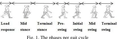
Walking is a complex motion. To allow quintic and cubic to represent a complete walking motion, the motion needs to be separated into several phases. Each phase will be represented by a quintic and cubic equation (see Figure 1).
Fig. 1. The phases per gait cycle
To achieve the smooth transition from one phase to another, the boundary conditions for the initial and final position, velocity and acceleration must be satisfied.
Related to quintic polynomial, the boundary conditions of initial and final position, velocity and acceleration must be satisfied in order to achieve a smooth transition from one phase to another as shown in Equation (7).
𝜃(𝑡0) = 𝜃0
𝜃̇(𝑡0) = 𝑣0
𝜃̈(𝑡0) = 𝑎0
𝜃(𝑡𝑓) = 𝜃𝑓
𝜃̇(𝑡𝑓) = 𝑣𝑓
𝜃̈(𝑡𝑓) = 𝑎𝑓
(7)
Related to cubic polynomial, the boundary conditions of initial and final position and velocity must be satisfied in order to achieve the smooth transition from one phase to another as shown in (8).
𝜃(𝑡0) = 𝜃0
𝜃̇(𝑡0) = 𝑣0
𝜃(𝑡𝑓) = 𝜃𝑓
𝜃̇(𝑡𝑓) = 𝑣𝑓
(8)
The coefficients value was stated in Table II and III obtained from the angular position, velocity, and acceleration values of real human walking for different sub phases of one gait cycle based on Table I.
Table I
Data of angular position, velocity, and acceleration for hip, knee, and ankle joint [24,25]. Sub-phases Time
instant Ankle joint
Knee joint
Hip joint Ang.pos
(D)
Ang.Vel (D/s)
Ang.Acc (D/s2)
Ang.pos (D)
Ang.Vel (D/s)
Ang.Acc (D/s2)
Ang.pos (D)
Ang.Vel (D/s)
Ang.Acc (D/s2)
Initial Contact 0% -26.217 0 0 4.3385 0 0 23.5332 0 0
Opp. Toe Off 10% -26.352 75.5274 868.2251 16.3274 50.8729 -2117.138 19.1885 -77.4824 -768.1465
Heel Rise 30% -15.353 35.5110 166.7023 7.8702 -48.7919 178.3133 -3.4331 -115.4348 147.4428
Opp. I.C. 50% -18.6765 -193.075 -3251.44 14.6468 130.5277 1099.215 -18.7007 -11.2649 1294.918
Toe Off 60% -42.7966 -148.097 4547.119 39.1988 328.1925 980.110 -10.5379 157.4401 1549.463
Feet Adjacent 73% -27.7267 170.506 -1852.074 59.8753 -72.599 -3871.23 13.9594 165.216 -894.0506
Tibia Vertical 87% -21.4686 -25.7715 -995.502 21.6284 -368.176 341.644 24.4748 -6.6616 -1019.859
Initial Contact 100% -25.9495 -32.6601 -1011.35 3.1826 118.317 2301.588 22.6209 -3.0761 -130.997
Table II
Coefficients value of the trajectory quintic polynomial for hip, knee, and ankle joint Gait
sub phase Time period
Joint a
0 a1 a2 a3 a4 a5
Loading
response 0-10%
Hip 23.53324 0 0 -16294.9181 186145.0195 -666429.9010
Knee 4.3385 0 0 88953.9003
-1230507.1592 4608569.0499 Ankle -26.2171 0 0 -27222.8241 462164.1159 -1912888.718
Mid stance
10-30%
Hip 22.2396 22.885333 -571.5698 57.7757 3704.7506 -5212.11926
Knee -1.7951 328.6538 -1551.8897 -345.9063 13119.572 -19008.1745
Ankle -18.6931 -378.4550 4972.1406 -24554.429 54772.1505 -45802.8317
Terminal stance
30-50%
Hip -131.21072 2146.65534 -12341.3470 33004.3163 -43523.1476 23013.6424
Knee -310.7935 4329.4906 -22320.4019 55060.6378 -65950.4204 31363.7464
Ankle -197.2944 2486.8953 -13537.3676 35665.9235 -43961.8946 19484.48425
Pre swing
50-60%
Hip -32379.9120 296116.5048
-1079272.9895 1959213.8847
-1772320.7938 639664.6495 Knee -48539.511 439381.4405
-1584971.6765 2848018.8954 -2549333.144 909994.1257 Ankle 15443.0507 -147189.712 553793.4104 -1027307.776 938387.3927 -337630.8437
Initial swing
60-73%
Hip 623.56690 -288.8231 -12050.6777 35252.287512 -36929.5445 13490.3278
Knee 66732.9741 -491709.060 1442496.1555 -2107834.384 1536454.9259 -447521.689
Ankle -97085.8257 738847.4255 -2234443.512 3356261.4122
-2504905.5189 743538.1714
Mid swing
73-87%
Hip 30540.86282 -190772.016 473402.2254 -584129.7203 358979.3023 -88018.1546
Knee 18834.1207 -122050.071 310760.5228 -387632.1367 237148.8847 -57077.6092
Ankle 86907.0625 -552428.767 1397199.0526 -1759314.837 1103583.2119 -276034.866
Terminal swing
87-100%
Hip -17895.0909 79904.3463 -137260.0977 111478.13999 -41201.73671 4997.05997
Knee -117563.742 575518.0644
Table III
Coefficients value of the trajectory cubic polynomial for hip, knee, and ankle joints
Gait sub phase Time period Joint a0 a1 a2 a3
Loading
response 0-10%
Hip 23.53324 0 -528.5904 941.1888
Knee 4.3385 0 3087.9335 -18890.4600
Ankle -26.2171 0 -795.8637 7823.3376
Mid stance 10-30%
Hip 22.6580 16.4176 -594.3727 832.4860
Knee 0.08320 295.6739 -1548.9531 2166.3183
Ankle -35.0099 97.8847 -115.7022 26.10207
Terminal stance 30-50%
Hip 19.569 20.5316 -518.8322 649.3808
Knee 43.9960 -160.6159 29.2177 349.2345
Ankle 90.4068 -1020.318 3158.4252 -3108.2434
Pre swing 50-60%
Hip 475.3589 -2391.9665 3661.6816 -1707.9735
Knee 721.6350 -3766.4354 6320.8289 -3231.8211
Ankle -2160.9076 12292.7582 -23078.1076 14123.03162
Initial swing 60-73%
Hip 824.0962 -4094.6877 6431.2749 -3208.7056
Knee 345.8889 -2681.9994 5837.25973 -3698.6294
Ankle 4033.9923 -17902.5689 25948.8159 -12392.6917
Mid swing 73-87%
Hip -646.8017 1871.7201 -1634.5197 425.27966
Knee -3148.7797 11734.8251 -13987.3939 5388.2349
Ankle -1939.9464 6572.9117 -7476.5644 2823.1554
Terminal swing 87-100%
Hip -855.2037 2870.1428 -3103.7355 1111.4173
Knee 140.1090 1615.1366 -3759.3694 2007.3065
Ankle -520.1295 1642.5675 -1769.9348 621.5474
Fig. 3. Comparing angular velocity profiles of both quintic and the cubic polynomials with reference trajectory profile related to ankle, knee, and hip joints.
3. RESULT AND DISCUSSION
In this part, the result of trajectory generation profiles of the ankle, knee, and hip joints has been generated based on both cubic and quintic polynomial equations. The result will be illustrated and demonstrated with further analysis and discussion. A generated trajectory profiles will be compared with real trajectory profile of human’s lower limb joints.
In this paper, both cubic and quintic polynomial equations are involved to create trajectory motion profiles. Comparison between both cubic and the quintic polynomials with human trajectory reference profiles will be explained with considering the analytical methods such as root mean square error (RMSE) and average difference error (ADE) as shown in (9) and (10).
𝑅𝑀𝑆𝐸 = √∑ (𝑇𝐺𝑒𝑛− 𝑇𝑅𝑒𝑓)2
𝑛 𝑖=1
𝑛 (9)
Average Difference =∑ ((𝑇𝐺𝑒𝑛− 𝑇𝑅𝑒𝑓)
𝑛 𝑖=1
𝑛 (10)
Where (TRef) is the reference trajectory, (TGen) is the generated trajectory and (n) is the number of trials.
The comparison leads to understanding either cubic or quintic accurately matches to real human trajectory profiles of lower limb joints.
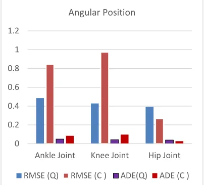
3.1 Angular Position
The angular position profile of all three lower limb joints (ankle, knee, and hip) are illustrated in Figure 2.
The RMSE and ADE have been calculated for all ankle, knee, and hip joint. The error is obtained based on the comparison between both cubic and the quintic polynomials with the real human trajectory profile of angular position according to ankle, knee and hip joints as illustrated in Table 4 and Figure 5.
Table 1V: RMSE and AD based on the angular position
Joint Method
Ankle (Degree) Knee (Degree) Hip (Degree)
RMSE ADE RMSE ADE RMSE ADE
Quintic 0.4852 0.0483 0.4283 0.0426 0.3917 0.0388
Cubic 0.8417 0.0838 0.9728 0.0968 0.2639 0.0263
3.2 Angular Velocity
The angular velocity profile of the three joint (ankle, knee, and hip) are generated based on quintic and cubic polynomial as shown in Figure 3.
Table 5 shows The RMSE and ADE that have been obtained for ankle, knee, and hip joints. The error is computed based on the comparison between both cubic and the quintic polynomial with the real human trajectory profile of angular velocity related to ankle, knee and hip joints.
Table V
RMSE and AD based on the angular velocity
Joint
Method
Ankle (D/s) Knee (D/s) Hip (D/s)
RMSE ADE RMSE ADE RMSE ADE
Quintic 1.7056 0.1697 12.007 1.1947 0.1659 0.0165
Cubic 1.4044 0.1397 5.3020 0.5275 0.1518 0.0151
0 2 4 6 8 10 12 14
Ankle Joint Knee Joint Hip Joint
Angular Velocity
RMSE(Q) RMSE(C )
ADE(Q) ADE(C )
Fig. 5. RMSE and ADE based on the angular position for the quintic (Q) and cubic (C) Polynomials.
0 0.2 0.4 0.6 0.8 1 1.2
Ankle Joint Knee Joint Hip Joint Angular Position
3.3 Angular Acceleration
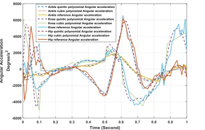
The angular acceleration profile of the ankle, knee, and hip joints are generated based on quintic and cubic polynomial as shown in figure 4.
Table VI shows The RMSE and ADE that have been calculated for ankle, knee, and hip joints. The error is computed based on the comparison between both cubic and the quintic polynomials with the real human trajectory profile of angular velocity for ankle, knee and hip joints.
Table VI
RMSE and AD based on the angular acceleration
Joint Method
Ankle (D/s2) Knee (D/s2) Hip (D/s2)
RMSE ADE RMSE ADE RMSE ADE
Quintic 65.83 6.55 21612.64 2150.54 5.5086 0.5481
Cubic 26.08 2.60 21460.48 2135.34 103.23 10.271
Fig. 7. RMSE and ADE based on the angular acceleration for the quintic (Q) and cubic (C) Polynomial.
Based on the root mean square error (RMSE), and average difference error (ADE), the error is less than 1 for all three joints either based on quintic or cubic polynomial.
In term of angular position, quintic polynomial generated trajectory profile of both ankle and knee joint with less RMSE and ADE compared to cubic polynomial trajectory profile.However, cubic polynomial generated hip trajectory profile with less the RMSE and ADE as illustrated in Figure 5 and Table 4.
The value of angular velocity and acceleration of cubic polynomial ( 3rd order) will be less compared to quintic polynomial (5th order) during generating the trajectory profile. This is due to the increasing number of polynomial order that will generate a smoother and accurate profiling position. On the other hand, the value of angular velocity and acceleration will be increased but it is still reasonable to be acceptable. We can make the comparison more obvious, Table 5 and 6 illustrate the RMSE and ADE of three lower joints based on quintic and cubic polynomial as shown in Figure 6 and 7.
generating angular position profile seems like quintic is the best. However, during velocity and acceleration, the cubic produces the more accurate profile. From my point of view, the quintic is accurate for position trajectory but not for velocity and acceleration.
3.4 Scaling in Time
In some cases, a trajectory must be modified in order to take into proper consideration the saturation limits of the actuation system and to plan the desired motion so that these limits are not violated. Motion profiles requiring values of velocity, acceleration, and torque outside the allowed ranges must be avoided since these motions cannot be performed.
Table VII and VIII show the maximum values of both velocity and acceleration based on stance and swing phases.
Table VII
VelocityMax of real human data
Value Joint
Max.vel
Stance swing
Ankle 99.3374 243.4051
Knee 310.294 339.7247
Hip 129.064 204.235
Table VIII
AccelerationMax of real human data
Value Joint
Max.Acc
Stance swing
Ankle 9656.563 8661.31
Knee 14980.56 6836.75
Hip 2068.377 2010.61
Related the cubic polynomial, the duration time of trajectory profile for both velocity and acceleration can be calculated based on equation 11 and 12 as shown in Table 9.
𝜃̇𝑚𝑎𝑥 =
3ℎ
2𝑇 → 𝑇 = 3ℎ 2𝜃̇𝑚𝑎𝑥
(11)
𝜃̈𝑚𝑎𝑥 =
6ℎ
𝑇2 → 𝑇 = √
6ℎ 𝜃̈𝑚𝑎𝑥
(12)
The duration time of quintic trajectory profile for both velocity and acceleration can be obtained based on the equation 13 and 14 as illustrated in Table 10.
𝜃̇𝑚𝑎𝑥 =
15ℎ
8𝑇 → 𝑇 =
15ℎ 8𝜃̇𝑚𝑎𝑥
(13)
𝜃̈𝑚𝑎𝑥 =
10√3ℎ
3𝑇2 → 𝑇 = √
10√3ℎ 3𝜃̈𝑚𝑎𝑥 (14) 0 5000 10000 15000 20000 25000
Ankle Joint Knee Joint Hip Joint
Angular Acceleration
Table IX
Duration time based on velocity max Time
Joint
Tvel .C Tvel .Q
Stance swing Stance swing Ankle 0.250 0.104 0.313 0.130
Knee 0.169 0.159 0.211 0.199
Hip 0.396 0.244 0.495 0.304
Table X
Duration time based on accelerationmax Time
Joint
Tacc .C Tacc .Q
Stance swing Stance swing
Ankle 0.102 0.108 0.10 0.106
Knee 0.118 0.178 0.116 0.174
Hip 0.314 0.315 0.308 0.309
According to Table 9 and 10, it is possible to see that in any case, the most restrictive constraint is due to the velocity limit and that, if the degree of the polynomial function increases, the duration T of the trajectory increases as well (the maximum velocity is fixed). This result has a general validity: given a maximum value for the velocity (or for the acceleration), the ‘smoother’ the motion profiles are, the longer the relative durations are.
4. CONCLUSION
To conclude that, in lower limb exoskeleton system, different trajectory methods have been used either off-line, on-line or both off-on-line and on-on-line. The quintic and cubic polynomials have been used to generate the trajectory for a different kind of robot, especially for the biped robot. In this paper, trajectory profiles of the quintic and cubic polynomials were compared to the real human trajectory profile. The purpose of this comparison is to analyze the ability to generate high accuracy profiling either by using quintic or cubic polynomial. The result shows that quintic generates the profile motion of all lower limb joints (ankle, knee, and hip) with 0.48520,0.42830, 0.39170 RMS error respectively. Meanwhile, cubic polynomial generated the trajectory motion profile of ankle, knee, hip joints with 0.84170, 0.97280, 0.26390 RMS error respectively. In conclusion, the quintic polynomial is better than cubic polynomial to generate the trajectory motion profile with smooth acceleration profile rather than linear as it occurs in the cubic polynomial. However, the complexity in designing the trajectory is increased. It can be stated that higher order of polynomial equation will provide higher accuracy in trajectory generation.
ACKNOWLEDGEMENT
The authors would like to thank for the support given to this research by Universiti Teknikal Malaysia Melaka (UTeM) and UTeM Zamalah Scheme. This project was conducted in Center of Excellence in Robotics and Industrial Automation (CERIA) in Universiti Teknikal Malaysia Melaka.
REFERENCES
[1] Xu, Yangsheng, and Ka Keung C. Lee,“HumanBehavior Learning and Transfer", CRC Press, 2005.
[2] A. Vakanski, I. Mantegh, A. Irish, and F. Janabi-Sharifi, Trajectory Learning for Robot Programming by Demonstration Using Hidden Markov Model and Dynamic Time Warping", IEEE Transactions on system, man, and cybernetics -part B: Cybernetics, Vol. 42, No. 4, 1039-1052, 2012.
[3] Y.Kuniyoshia, Y.Ohmuraa, K.Teradaa, A.Nagakuboc, S.Eitokua, T.Yamamotob, “Embodied basis of invariant features in execution and perception of whole-body dynamic actions-knacks and focuses of Rolland-Rise motion", Robotics and Autonomous Systems, Vol.48, No.4, 189-201, 2004.
[4] Z.Wang, H. B.Amor, D.Vogt, J.Peters, “Probabilistic movement modeling for intention inference in human-robot interaction”, International Journal of Robotics Research, Vol.32, No.7, 841-858, 2013.
[5] E.Gribovskaya, S.M.Khansari-Zadeh, A.Billard, “Learning Non-linear Multivariate Dynamics of Motion in Robotic Manipulators”, International Journal of Robotics Research, Vol.30 No.1, 80-117, 2011.
[6] Razali MR, Miskon MF, bin Bahar MB, The influence of the swaying arm angle range to the torso torque of the humanoid robot during walking. In Robotics and Intelligent Sensors (IRIS), 2015 Oct 18 (pp. 93-98).
[7] J.V.D.Berg, S.Miller, D.Duckworth, H.Hu, A.Wan, X.Fu, K.Goldberg,"P.Abbeel, Superhuman Performance of Surgical Tasks by Robots using Iterative Learning from Human-Guided Demonstrations”, IEEE International Conference on Robotics and Automation, Anchorage, Alaska, USA, 2074-2081, 2010. [8] J.Peters, S.Schaal, “Learning to Control in Operational Space”,
International Journal of Robotics Research, Vol.27, No.2, 197-212, 2008.
[9] Garrido, Javier, and Wen Yu. "Trajectory generation in joint space using modified hidden Markov model." In Robot and Human Interactive Communication, 2014 RO-MAN: The 23rd IEEE International Symposium on, pp. 429-434, 2014.
[10] Miskon, Muhammad Fahmi Bin, and Muhammad Bin Abdul Jalil Yusof. "Review of trajectory generation of exoskeleton robots." In Robotics and Manufacturing Automation (ROMA), 2014 IEEE International Symposium on, pp. 12-17, 2014.
[11] Craig, John J. Introduction to robotics: mechanics and control. Vol. 3. Upper Saddle River: Pearson Prentice Hall, 2005.
[12] Biagiotti, Luigi, and Claudio Melchiorri. Trajectory planning for automatic machines and robots. Springer Science & Business Media, 2008.
[13] Cuevas, Erik, Daniel Zaldivar, Marco Perez, and Marte Ramirez. "Polynomial trajectory algorithm for a biped robot." arXiv preprint arXiv: 1405.5937 (2014).
[14] Haghighi, HR Elahi, and M. A. Nekoui. "Inverse kinematic for an 8 degrees of freedom biped robot based on cubic polynomial trajectory generation." In Control, Instrumentation and Automation (ICCIA), 2011 2nd International Conference on, pp. 935-940, 2011.
[15] Tang, Zhe, Changjiu Zhou, and Zenqi Sun. "Trajectory planning for smooth transition of a biped robot." In Robotics and Automation, 2003. Proceedings. ICRA'03. IEEE International Conference on, vol. 2, pp. 2455-2460. IEEE, 2003.
[16] Bahar MB, Miskon MF, Bakar NA, Ali F, Shukor AZ, Sts motion control using humanoid robot, Research Journal of Applied Sciences, Engineering and Technology, 2014 Jul 5;8(1):95-108. [17] Ali, Sari Abdo, Khalil Azha Mohd Annuar, and Muhammad Fahmi
Miskon. "Trajectory Planning For Exoskeleton Robot By Using Cubic And Quintic Polynomial Equation." International Journal of Applied Engineering Research 11, no. 13 (2016): 7943-7946. [18] Rai, J. K., R. P. Tewari, and Dinesh Chandra. "Trajectory planning
Journal of Telecommunication, Electronic and Computer Engineering (JTEC) 8, no. 7 (2016): 151-155.
[20] Sciavicco, Lorenzo, and Bruno Siciliano. Modelling and control of robot manipulators. Springer Science & Business Media, 2012. [21] Siciliano, Bruno, Lorenzo Sciavicco, Luigi Villani, and Giuseppe
Oriolo. Robotics: modelling, planning and control. Springer Science & Business Media, 2010..
[22] Jazar, Reza N. Theory of applied robotics: kinematics, dynamics, and control. Springer Science & Business Media, 2010.
[23] Rai, Jaynendra Kumar, and Ravi Tewari. "Quintic polynomial trajectory of biped robot for human-like walking." In Communications, Control and Signal Processing (ISCCSP), 2014 6th International Symposium on, pp. 360-363, 2014.
[24] Bovi, G., Rabuffetti, M., Mazzoleni, P. and Ferrarin, M.,”A multiple-task gait analysis approach: kinematic, kinetic and EMG reference data for healthy young and adult subjects. Gait & posture”, 33(1), pp.6-13, 2011.