Modeling and Analysis of the Dynamic Performance of a Robot Manipulator driving by an Electrical Ac- tuator Using Bond Graph Methodology

Modeling and Analysis of the Dynamic Performance

of a Robot Manipulator driving by an Electrical

Ac-tuator Using Bond Graph Methodology

Fatima Zahra Baghli

, Larbi El bakkali

1

Modeling and Simulation of Mechanical Systems Laboratory, Abdelmalek Essaadi University, Faculty of Sciences, BP.2121, M’hannech, 93002, Tetuan, Morocco

*Corresponding author: Tel.: +212644989050, Fax: +212539994500, E-mail address: [email protected] Abstract-- In this present paper we propose a new approach for

modeling a rigid multibody system based on Bond Graph method-ology. The proposed method based on the transfer of energy be-tween system components and on the description of the vector ve-locity relation of a moving point in a rotating system.

Our mechatronic system is a double freedom robot manipulator driving by an electric actuator, can be efficiently modeled and solved by this multidisciplinary approach, this design of bond graph dynamic model of the arm manipulator derive information on structural controllability and observability. Also the advantages of bond graph modeling of the robot manipulator are notified.

Index Term-- Bond graph, Dynamic modeling, and Robot ma-nipulator.

1. INTRODUCTION

Research on the dynamic modeling and simulation of the arms manipulators has received increased attention since the last years due to their advantages, this system is a mechanical system mul-ti-articulated, in which each articulation is driven individually by an electric actuator is the most robot used in industry. A good modeling of the specific manipulator needs an efficient method to describe all behaviors of system.

The Newton-Euler technique and Lagrange‟s technique are the most methods used for dynamic modeling; these techniques calculate a vector containing the force or torque required at each joint to attain a specified trajectory of joint positions, velocities and accelerations. The main disadvantages of the above model-ing techniques are their complexity and lack of versatility [1].

The Bond Graph technique developed since the 1960's repre-sent a powerful approach to modeling robotic manipulators and mechanisms [2-3].It is a graphical representation that depicts the interaction between elements of the system along with their cause and effect relationships. The use of Bond Graph to de-scribe all behaviors of robotic manipulators can he developed based on kinematic relationships between the time rates of joint variables and the generalized Cartesian velocities (translational and angular velocities) [1].This efficient method can be used to

obtain more information such as the power required to drive each joint actuator, or the power interaction at the interface with the environment, Such information can also be used to study the performances like stability, precision of the manipulator system.

In this work the study is extended to a highly non linear, mul-tiple inputs mulmul-tiple outputs (MIMO) system, this study is illus-trated by the two arms manipulator. The aim of this work is to describe all behaviors of our system by using bond graphs.

The reminder paper was structured as follow: the Bond graph technique for modeling a mechanical and electrical system has been presented in second part of this paper, in the third part of this paper the systematic procedure to derive a Bond Graph is detailed, The equations of motion are derived from Bond graph model with the criteria of controller such as controllability and observability are presented in the last part of this paper and final-ly conclusion was given.

2. BOND GRAPH OF MECHANICAL AND ELECTRICAL SYSTEM

2.1 Bonds

International Journal of Mechanical & Mechatronics Engineering IJMME-IJENS Vol:14 No:04 75

Fig.1. Energy bond with effort and flow

Table I gives examples of the effort and flow variables for mechanical and electrical domains.

Table I

Effort and Flow variables in some physical domains

Domain Effort (e) Flow (f)

Translation Mechanics Force Velocity

Rotational Mechanics Torque Angular velocity

Electricity Voltage Current

2.2 Components

There are four types of components labeled S, C, I, R, this ele-mentary components are classified by their energetic behavior

(en-ergy dissipation, en(en-ergy storage, etc.) and define how the effort and flow variables on the bond relate to each other. The Table 2 shows the elementary component of bond graph.

Table II .Basic Bond Graph elements Component Symbol Type of element Example in translation

mechanic domain

Example in rotational mechanic domain

Example in electric domain

Active ele-ments

Se Effort source Force source Torque source Voltage source Sf Flow source Velocity source Angular velocity

source

Current source

Passive ele-ments

R Dissipation Damper Rot. Damper Resistor

I

Storage

Inertia Rot. Inertia Inductor

C Compliance Rot. Compliance Capacitor

2.3 Junctions

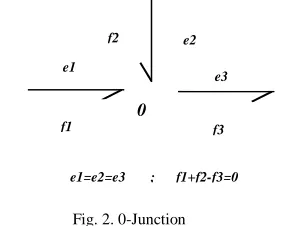
The Components are connected together using two types of junc-tions: a 0 or common effort junction and a 1 or common flow junc-tion.

The 0 junction has the following properties: all bonds impinging

upon it have the same effort variable and all flows on attached bonds sum to zero. Similarly the 1 junction has the properties: all bonds impinging upon it have the same flow variable and all ef-fort on attached bonds sum to zero

Fig. 2. 0-Junction Fig. 3. 1-Junction

2.4 Connecting mechanical and electrical domains

To transfer between physical domains the ability to multiply must be included and bond graph provide two means of accom-plishing this: the Transformer TF and the Gyrator Gy (TF or Gy are energy conserving).

Symbol Mechanical domain Electrical domain

TF Lever Transformer

Gy Gyroscope Motor Dc

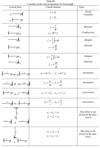
2.4 Determining causality:

Bond graphs have a notion of causality, indicating which side of a bond determines the instantaneous effort and which deter-mines the instantaneous flow. In formulating the dynamic equa-tions that describe the system, causality defines, for each model-ing element, which variable is dependent and which is independ-ent.

The sources Se and Sf have fixed causality because there can

e1

1

f1=f2=f3 ; e1+e2-e3=0

e2

e2 e3 f3 f1

f2 e1

0

e1=e2=e3 ; f1+f2-f3=0

e2

e2 e3 f3 f1

f2

e

be only one output variable in relation to the source.

Storage elements C, I have “preferred causality”, the advantage is given to the integral causality over the differential one consid-ering the fact that these elements are characterized by effort and flow accumulation which is manifested by the mechanism of integration in time, the rest of elements, as the element of dissi-pation R, have the so called “free causality‟‟ because they repre-sent only static connection between the effort and the flow, The junction 1 has only one independent flow variable and only one

bond with causal stroke which is not on the side of the element In the same way, 0 junction has only one independent effort var-iable, and only one bond with causal stroke towards the ele-ment of this connection. Therefore, Transformers and gyrators also have causal constraints. Table 3 shows the permitted causal-ity permutations for components, junctions and transformers respectively.

Table III

Causality stroke and Assignments for bond graph

Causal form Causal relation Type

e

eS

f

f S

Fixed Causality

e f

R



*

eR f

Resistor

Conductivity

1

f e dt

I



_

df

e I

dt



Integral

Derived

1

e f dt

C



_

de

f I

dt



Integral

Derived

1 * 2 ; 2 * 1

e m e f m f Symmetric

1 2

2 ; 1

e f

e f

m m

  Symmetric

1 * 2 ; 2 * 1

e r f e r f Antsymmetric

1 2

2 ; 2

e e

f f

r r

  Antsymmetric

2 3 1

1 2 3

e e e

f f f

 

 

One effort is im-posed on the

junc-tion 0

2 3 1

1 2 3

f f f

e e e

 

 

One flow is im-posed on the

junc-tion 1

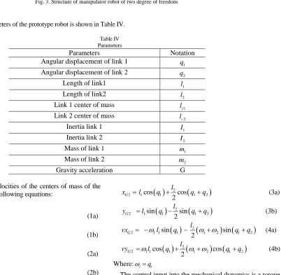
3.DESCRIPTION OF THE ROBOT MANIPULATOR

In this section, geometric and kinematic models are used for modeling the behavior of a robot manipulator with 2DOF.

The parameters of the system are joint and operational positions, the first allows modifying its geometry and the second determines the

position and the orientation of the end effector M. In Fig. 3 a sche-ma is given of 2-link rigid arm in which each articulation is driven individually by an electric actuator:

Sf

Se

1

1 2

3

0

1 2

3 1

Gy : r 2

1

Gy : r 2

1

TF :m 2

1

TF : m

International Journal of Mechanical & Mechatronics Engineering IJMME-IJENS Vol:14 No:04 77

Fig. 3. Structure of manipulator robot of two degree of freedom

The meaning of the parameters of the prototype robot is shown in Table IV.

Table IV Parameters

Parameters Notation

Angular displacement of link 1

1 q Angular displacement of link 2

2 q Length of link1

1 l Length of link2

2 l

Link 1 center of mass l_c1

Link 2 center of mass

2 c l Inertia link 1

1 I

Inertia link 2 I₂

Mass of link 1

1 m Mass of link 2

2 m

Gravity acceleration G

The positions and the velocities of the centers of mass of the two links are described by following equations:

 

1 cos 1

2 G

l

x  q (1a)

 

1 sin 1

2 G

l

y  q (1b)

 

1 1 sin 1

2 G

l

vx   q (2a)

 

1 1 cos 1

2 G

l

vy  q (2b)

 





2 1cos 1 cos 1 2

2 G

l

x l q  q q (3a)

 





2 1sin 1 sin 1 2

2 G

l

y l q  q q (3b)

 



 



2 1 1sin 1 1 2 sin 1 2

2 G

l

vx  l q    q q (4a)

 



 



2 1 1cos 1 1 2 cos 1 2

2 G

l

vy l q    q q (4b)

Where:_iq_i

The control input into the mechanical dynamics is a torque in-put. However an electrical dynamic system from voltage to torque needs to be derived.

2

G

y

l

2

q

1

q

2

l

y

0

x

x

y

g

M

1

G

y

2

G

x

G

x

1





2

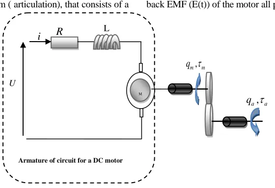
The following Fig.4 describe the circuitry within the DC motor system entrained joint robot arm ( articulation), that consists of a

resistor R, an inductor L, an external voltage source U, and a back EMF (E(t)) of the motor all placed in a series circuit.

Fig. 4. schematic model of single joint robot arm driven by an armature controlled DC motor

The variable common to all the components of the armature circuit of DC motor is the current i, by using Kirchoff‟s voltage law, the external source voltage is equal to the sum of the indi-vidual voltages across each circuit component as shown in the following equation:

( ) ( ) ( ) di t ( )

U t Ri t L E t

dt

   (5)

The torque produced by a DC. motor is given by:

1 ( ) m i t k

  (6)

So, the torque applied to the rotational base in the robot manipu-lator is converted to the torque applied by the DC motor by means of a gear ratio k2 given in the following equation:

2

a k m

   (7)

4.CLASSICAL MODELING OF ARM MANIPULATOR:

The dynamic equations of the robot are usually

repre-sented by the following Lagrange method

( ) ( , ) ( )

M q q C q q G q

   

(8)

Where:

, , n

q q q

denotes the joint angle, the joint velocity and

the joint acceleration,

M q  

is the manipulator

iner-tia matrix,

C q q  

is the centrifugal and Coriolis

force matrix,

G q 

is the gravitational force vector and

( )t



denotes the torque.

The robot dynamics is defined as:





2 2 2 2

1 2 1 1 2 1 2 2 1 2 2 2 2 2 2 1 2 2

2 2

2 22 2 1 2 2 2 22

2

( ) c c c c

c c

I I m l m l l m l l c I m l m l l c

M q

I m l m l l c I m l

        

 _ _

  

 

8a)

2 1 2 2 2 2 1 2 1 1 2

2 2 1 21 2

( )

( , )

0

c c

m l l q s m l l q q s

C q q

m l l q s

  

 

  

 

(8b)

1 1 2 1 1 2 2 12

2 2 12

( )

( ) c c

c

m l m l gc m gl c

G q

m gl c

 

 

  

 

(8c)

1

2  



      

(8b)

Where: 1 cos( )1

c  q ; c₂ cos(q₂) ; s₁sin( )q₁ ;

2 sin( 2)

s  q ;c₁₂ cos(q₁q₂) ; s₁₂sin(q₁q₂)

5.SYSTEMATIC PROCEDURE TO DERIVE A BOND GRAPH MODEL OF SYSTEM

The representation of the robot manipulator is developed by assembling bond graph represent of the different elements as shown in the word bond graph (Fig. 5)

Fig. 5. Robot manipulator word bond graph with boundary conditions (Sfi)

R

Armature of circuit for a DC motor

M

L

U

i

,

a a

q



,

m m

q



dc motor 1

dc motor 1

arm1 arm2

dc motor 2

f1

S S_f2

International Journal of Mechanical & Mechatronics Engineering IJMME-IJENS Vol:14 No:04 79

5.1.Bond graph for a DC motor

The DC motor is simply modeled by a gyrator (GY) for the electromechanical conversion, with a proportional gain k1.The bond graph of the armature will be constructed around a com-mon flow (because the variable comcom-mon to all the components is the current i). Connected to this junction will be a Source of voltage (Se), Inertia (I) corresponding to the armature inductance L and a Resistance (R) corresponding to the armature resistance R. The components to be added are the motor inertia Jm and the viscous friction b, to form the final version of the bond graph of Dc Motor shown in Fig. 6.

Fig. 6. Bond graph for DC motor

An integral causality is imposed when I and c components have the form as show in table. III

The causally complete Bond graph as shown in Fig. 7

Fig. 7. Causally bond graph for DC motor

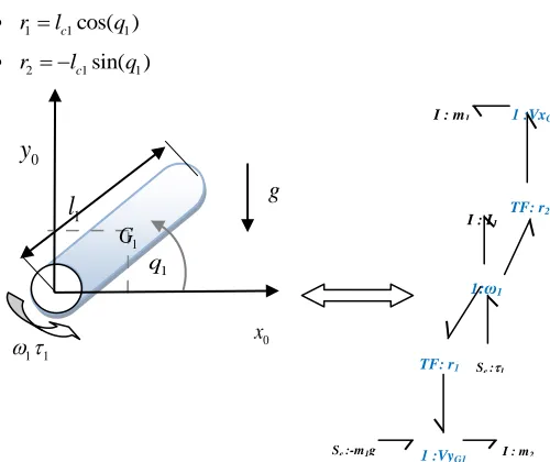
5.2.Bond graph for a rotating arm

The bond graph for the first arm is derived from expressions of the velocities of the center of mass Eq. (2a) and (2b).

The transformers are used to convert the angular velocity to a linear velocity and the dynamics can be introduced by adding I

element to the arm as shown in Fig .8. Where:

 r₁lc₁cos( )q₁

 r₂ lc₁sin( )q₁

Fig. 8. Bond graph for rotating of the first arm

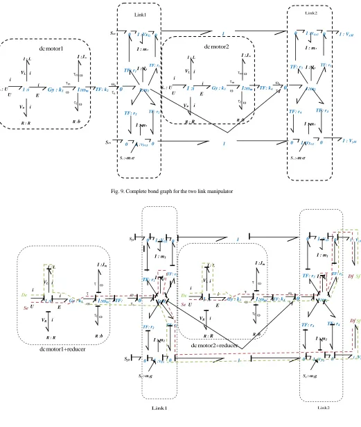
The base of the second arm is not fixed in space but depends on the velocity of its attachment point to the first arm, therefore, the development of the first and the second arm based on the expressions of the velocities of center mass of the second link Eq. (4a) and Eq. (4b).So, the complete bond graph of our system is shown in Fig 9.

Where:

 r₃ lc₂sin(q₂)

 r₄lc₂cos(q₂)

6. STRUCTURAL STUDY

The bond graph causal model is considered as a structural model and we synthesis this last one by tracking into account control criteria (controllability and observability).

In terms of bond graphs, the notions of input reachable and out-put reachable are expressed as the existence of causal paths be-tween dynamical elements (I, C in integral causality) and sources and detectors [9].

1 :VyG1 1:ω1

I : m1

Se :1 TF: r2

TF: r1

1 :VxG1

I : m2

Se :-m1g

I : I1

0 x

0

y

1

l

1 q 1 G

g

1 1

 

U

1 :i

i

VR

1:ωm

I : L

ωm

i i VL

i E

Gy : k1

m

R : R Se : U

m

f _ω m

ωm

TF: k2

R :b I :Jm

ωa a

1:ωa

U

1 :i

i

VR

1:ωm

I : L

ωm

i i VL

i E

Gy : k1

m

R : R Se : U

m

f ω m

ωm

TF: k2

R :b I :Jm

1 :VyG

1 1:ω1

I : m1

TF: r1

TF: r2 1 :VG1

I : m1

Se :-m1g

I : J1

TF: r1

TF: r2

0 0

Sf1

0 0

Sf2 1 :VyG

2 1:ω2

I : m1

1 :VGx

2

I : m1

I : J1

0

0

Se :-m2g

TF: r3 TF: r3

TF: r4 TF: r4

0 0

1 1

1 : VyM

1 : VxM

Link2

dcmotor1+reducer dc motor2+reducer

U

1 :i

i

VR

1:ωm I : L

ω m i i VL i E

Gy :k1



m

R : R

Se



m

f _ω

m

ω

m

TF:

k2

R :b I :Jm

ω

a a 0

Df Df U 1 :i i VR 1:ωm I : L

ω m i i VL i E

Gy : k3



m

R : R

Se



m

f ω

m

ω

m

TF: k4

R :b I :Jm

ω

a a 0

De Sf De Sf Link1 U 1 :i i VR 1:ωm I : L

ω m i i VL i E

Gy : k1

m

R : R

Se : U

m

f ω

m

ω

m _{TF: k}

2

R :b I :Jm

ωa a 0

1 :VyG1 1:ω1

I : m1

TF: r1

TF: r2 1 :VxG

1

I : m1

Se :-m1g

I : J1

TF: r1

TF: r2

0 0

Sf1

0 0

Sf2 1 :VyG2

1:ω2

I : m1

1 :VGx2

I : m1

I : J1

0 0 U 1 :i i VR 1:ωm I : L

ω m i i VL i E

Gy : k3

m

R : R Se : U

m

f ω

m

ω

m _{TF: k}

4

R :b I :Jm

ωa a 0

Se :-m2g

TF: r3 TF: r3

TF: r4 TF: r4

0 0

1 1

1 : VyM 1 : VxM

Link1 Link2

dc motor1 dc motor2

Fig. 9. Complete bond graph for the two link manipulator

International Journal of Mechanical & Mechatronics Engineering IJMME-IJENS Vol:14 No:04 81 Theorem 1: A system is structurally state controllable if all

dynamical elements (I, C) in integral causality are causally con-nected with a source (Se, Sf).

Theorem 2: A system is structurally state observable if all dy-namical elements (I, C) in integral causality are causally con-nected with a detector (De, Df).

6.1.Consideration of controllability and observability

To put the model of our system in model BGD, it is necessary to make all storage elements in integral causality. Thus the crite-rion of controllability is verified with the two sources U1 and U2 as shown in Fig. 10.

To ensure the observability, it is necessary to verify the exist-ence of a causal path between every Detectors and a dynamic element I and making all the dynamic element in complete cau-sality, in our bond graph model there is a causal way between the dynamic element I in integral causality and the output so the system is structurally observable with the two detectoes De or Df as shown in Fig. 10.

After verifying structurally our model, we pass to the follow-ing step with consists in makfollow-ing a study behavioral of our system with the objective deriving the dynamic equations of our system

from the bond graph model

7.Systematic procedure to derive the equation of motion from bond graph model

The simplified bond graph model of the robot manipulator can be represented as shown in Fig.11.

Where:

1 1 1

2 1 1

3 1 1 2 1 2

4 2 1 2

5 2 1 2

6 1 1 2 1 2

sin( ) cos( )

sin( ) sin( )

sin( )

cos( )

cos( ) cos( )

c c c c c c

k l q

k l q

k l q l q q

k l q q

k l q q

k l q l q q

                   

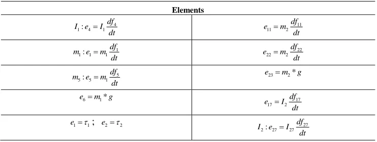
The junction equations and elements are illustrated in Tables V and Table VI

Table V

The junctions characteristic

Junction1 Junction 0 TF

1 3 4 8 10 14 26

1 3 4 8 10 14 26

0 1: e e e e e e e

f f f f f f f

      



       

25 26 27 26 27 25

0 :

0

e e e

f f f

 



 _{  }



3 1 18 1

18 1 3

* :

*

e k e

TF k

f k f

   _  9 18 18 9 1: 0 f f e e    _{ } 

13 12 15 15 13 12

0 :

0

e e e

f f f

 



 _{  }



8 2 7

2 18 1 3

* :

*

e k e

TF k

f k f

 

 _



5 6 7

6 7 5

1:

0

f f f

e e e

 



    

20 21 24 20 24 21

0 :

0

e e e

f f f

 



 _{  }



14 3 13 3

13 3 14

* :

*

e k e

TF k

f k f

     12 11 12 11 1: 0 f f e e    _{ }  -

16 4 15 4

15 4 15

* :

*

e k e

TF k

f k f

    

2 16 17 19 25 25 16 17 2 19

0 1: e e e e e

f f f f f

    



 _{   }

 -

19 5 20 5

20 5 19

* :

*

e k e

TF k

f k f

 

 _



21 23 22 21 22 23

0 1: e e e

f f f

  



 _{ }



10 6 24 6

24 6 10

* :

*

e k e

TF k

f k f

Fig. 11. Simplified Causally Bond Graph for the two link manipulator

Table VI

The equations of elements

Elements

4 1: 4 1

df

I e I

dt

 11

11 2

df

e m

dt



1 1: 1 1

df

m e m

dt

 22

22 2

df

e m

dt



5 5: 5 1

df

m e m

dt

 e23m2*g

6 1*

e m g 17

17 2 df

e I

dt



1 1

e  ; e22 27

2: 27 27 df

I e I

dt



1 :VyG1 1:ω1

I : m1

Se : 1

TF: k1

TF: k2

1 :VxG1

I : m2

Se :-m1g

I : I1

TF: k3 0 1 :VxG2

I : m2

1:ω2

Se : 2 TF: k6

I : I2

0

TF: k5 0 1 :VyG2

I : m2

TF: k4

Se :-m2g

I : I2

9

18

3 1

8 4

26

13

11 12 14

10

27

6 7

5

2

19 17

20 21

16 25

15

24

International Journal of Mechanical & Mechatronics Engineering IJMME-IJENS Vol:14 No:04 83 The torque applied to move link 1 can be obtained from the

bond graph by the Eq. (9) and the external torque applied to move the second link by the Eq. (10).

1 e1 e3 e4 e8 e10 e14 e26

       

(9)

2 e2 e16 e17 e19 e25

     

(10)

From the bond graph model and the precedent junction equa-tions and elements we can formulate a set of manipulator robot differential equations in the following matrix form:

1 11 12 1 11 12 1 1

2 21 22 2 21 22 2 2

( ) ( ) ( , ) ( , ) ( )

( ) ( ) ( , ) ( , ) ( )

M q M q q C q q C q q q G q

M q M q q C q q C q q q G q

 

           

  

           

           

(11) Where:

The elements of the inertia matrix M (q) in the terms of the pa-rameters of the robot manipulator are given by:

2 2 2

11( ) 1 2 1 1c 2c2 2 1 2 2 1c2 2

M q   I I m l m l m l  m l l c

2

12( ) 21( ) 2 2c2 2 2 1c2 2

M q M q I m l  m l l c 2

22( ) 2 2 2c2

M q  I m l

The matrix elements C q q i jij( , )( , 1,2) centrifugal and Cori-olis force are:

11( , ) 2 1c2 2 2 C q q  m l l q s

12( , ) 2 1c2 2( 1 2) C q q  m l l s q q

21( , ) 2 1c2 1 2 C q q m l l q s

22( , ) 0 C q q 

Finally the elements of the vector of gravitational torques G (q) are given by:

1( ) ( 1 2) c1 1 2 c2 12

G q  m m gl c m gl c

2( ) 2 c2 12

G q m gl c

The equations of external torque given by bond graph ap-proach correspond to those obtained using Lagrange methods, as illustrated in Eq. (8).

This indicates that, the model developed capture the essential aspects of rigid body dynamics of the robot manipulator. 8.CONTROLLER DESIGN

The general equation of the robot manipulator would be:

 

 

 

, q d q

q M q C q q G q

dt  

 

    

     

    

(12)

Robot control is the spine of robotics. It consists in studying how to make a robot manipulator do what it is desired to do automatically.

The dynamic model that characterizes the behavior of robot manipulators and obtained by bond graph is in general composed of nonlinear functions of the state variables (joint positions and velocities). This feature of the dynamic model might lead us to believe that given any controller.

The Fig.12 shows a block-diagram corresponding to a robot ma-nipulator under feedforward control

Fig. 12. Block-diagram of a robot manipulator

 

q

M

desired

q

desired q

desired

q



q



q

+



q

q



C

,



 

G

Robot

Manipulator

The state space equations Eq. (12) for this mechanical system have been derived. Solution these equations we can obtaine for example in MATLAB/Simulink.

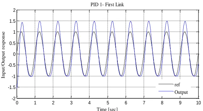
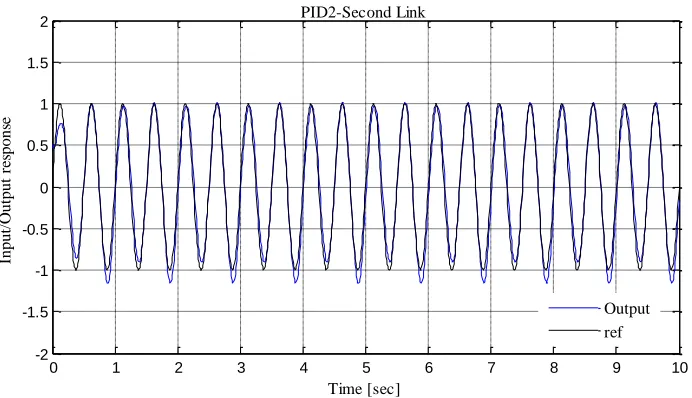
9. SIMULATION

SISO control based on classical PID model is tested to sinus

response trajectory [11]. This simulation applied to two degrees of freedom robot arm was implemented in Matlab/Simulink. The simulation results are illustrated by the following figures.

Fig. 13. Arm manipulator robot classical PID control

0 1 2 3 4 5 6 7 8 9 10

-2 -1.5 -1 -0.5 0 0.5 1 1.5 2

Time [sec]

Inp

ut

/O

ut

pu

t

re

spo

ns

e

PID 1- First Link

ref Output

Fig. 14. PID (First link trajectory) Arm Manipulator 1

( )

t



2

( )

t



* 2

q

* 1

q

q

2

q

PID 2

PID1

1

( )

t



2

( )

t

International Journal of Mechanical & Mechatronics Engineering IJMME-IJENS Vol:14 No:04 85

0 1 2 3 4 5 6 7 8 9 10

-2 -1.5 -1 -0.5 0 0.5 1 1.5 2

Time [sec]

Inp

ut

/O

ut

pu

t

re

spo

ns

e

PID2-Second Link

Output ref

Fig. 15. PID (Second link trajectory)

10. CONCLUSIONS

In this paper, a new approach for modeling a robot manipula-tor is proposed, the proposed method is a concise and uniform language for the description of physical systems.

The modeling of our system using bond graph offers some useful advantages:

First, Ability to create bond graphs of large, complex system by connecting the bond graphs of simple sub-system.

Second, Graphical format is constructed through consideration of the kinematics of the robot manipulator.

Third, Dynamic equations of motion derived automatically from the causally complete bond graph of the two link manipulator.

Bond graph method combined with computer implementation is a very powerful tool for modeling and simulation of dynamic systems.

ACKNOWLEDGEMENTS

The authors would like to thank Oussama Khatib, Professor of Computer Science at Stanford University, California.

ABREVIATIONS BGI : Bond graph in integral causality BGD : Bond graph in derivative causality De : Detector of effort

Df : Detector of flow Sf : Flow source Se : Effort source

EMF: Back electromotive force

REFERENCES

[1] Anand Vaz, Harmesh Kansal and Ani1 Singla, Some Aspects in the Bond Graph Modelling of Robotic Manipulators: Angular Velocities from Sym-bolic Manipulation of Rotation Matrices, IEEE 2003.

[2] Darina Hroncováa, Patrik Šargaa, Alexander Gmiterkoa, Simulation of mechanical system with two degrees of freedom with Bond Graphs and MATLAB/Simulink, Procedia Engineering 48 ( 2012 ) 223 – 232.

[3] Wolfgang Borutzky, Bond Graph Methodology: Development and Analysis of Multi-disciplinary Dynamic System Models, Springer 2010.

[4] Soo-Jin Lee1, Pyung-Hun Chang, Modeling of a hydraulic excavator based on bond graph method and its parameter estimation, Journal of Mechanical Science and Technology 26 (1) (2012) 195~204 .

[5] Tore Bakka and Hamid Reza Karimi, Bond graph modeling and simulation of wind turbine systems, Journal of Mechanical Science and Technology 27 (6) (2013) 1843~1852.

[6] Dragan Antic, Biljana Vidojkovic and Miljana Mladenovic, An Introduc-tion to Bond Graph Modelling of Dynamic Systems, TELSIKS'99 13-1 5.October 1999, NiS, Yugoslavia

[7] MA. Malik , A. Khurshid, Bond Graph Modeling and Simulation of„ Mech-atronic Systems, Proceedings IEEE INMIC 2003.

[8] C. Sueur, G.Dauphin-Tanguy Bond-graph Approach for Structural Analysis of MIMO Linear Systems, Journal of the Frankhn Institute Pergamon Vol. 328, No. 1, pp. 55-70, 1991.

[9] M.H. Toufighi, S.H. Sadati, F. Najafi Modeling and Analysis of a Mecha-tronic Actuator System by Using Bond Graph Methodology IEEE. January 13, 2007.

[10] Fatima Zahra Baghli, Larbi El bakkali, Yassine Lakhal, Abdelfatah Nasri, Brahim Gasbaoui, «The efficiency of the inference system knowledge strat-egy for the position control of a robot manipulator with two degree of free-dom», International Journal of Research in Engineering and Technology, Volume: 02 Issue: 07 Jul-2013.

[11]Fatima Zahra Baghli, Larbi El Bakkali,Yassine Lakhal,Abdelfatah Nasri, Brahim Gasbaoui, “Arm manipulator position Control based on Multi-Input Multi-Output PID Strategy”, Journal of Automation, Mobile Robotics & In-telligent Systems , volume 8, N° 2, 2014.