Abstract—To reduce the overall time of structural
optimization for earthquake loads two strategies are adopted. In the first strategy, a neural system consisting self-organizing map and radial basis function neural networks, is utilized to predict the time history responses. In this case, the input space is classified by employing a self-organizing map neural network. Then a distinct RBF neural network is trained in each class. In the second strategy, an improved genetic algorithm is employed to find the optimum design. A 72-bar space truss is designed for optimal weight using exact and approximate analysis for the El Centro (S-E 1940) earthquake loading. The numerical results demonstrate the computational advantages and effectiveness of the proposed method.
Index Terms—Optimization, genetic algorithm, earthquake,
neural networks, self-organizing map, radial basis function.
I. INTRODUCTION
Optimum design of structures is usually achieved by selecting the design variables such that an objective function is minimised while all of the design constraints are satisfied. Structural optimization requires that the structural analysis to be performed many times for the specified external loads. This makes the optimal design process inefficient, especially when a time history analysis is considered. This difficulty will be resonated when the employed optimization method has the stochastic nature such as evolutionary algorithms.
In the recent years, traditional and evolutionary search techniques were employed to optimal design of structures subjected to response spectrum and earthquake loadings. Salajegheh and Heidari [1] incorporated neural network techniques in the optimization process to predict structural time history responses. They employed wavelet back propagation neural network. In the recent years, neural networks are broadly utilized in civil and structural engineering applications.
In this investigation, in order to eliminate the drawback, the dynamic responses of the structures have been approximated using a self-organizing neural system.
S. Gholizadeh and E. Salajegheh introduced an intelligent neural system (INS) for efficient approximation of time history structural responses in Ref. [2]. In INS, the input and target spaces are divided into some subspaces as the data located in each subspace have similar properties. These properties are taken as significant natural periods of the structures. Classification of input space is achieved by using competitive neural networks. Then a distinct radial basis function (RBF) neural network is trained for each subspace
Manuscript received October 30, 2014; revised February 27, 2015. Alireza Lavaei and Alireza Lohrasbi are with Department of Civil engineering, College of engineering, Boroujerd Branch, Islamic Azad University, Iran (e-mail: [email protected], [email protected]).
using its assigned training data. Also, the authors incorporated the INS in the optimization process in Ref. [3]. The numerical results showed great computational efficiency with a main limitation of difficulties for determining the number of data clusters.
In the present study, self-organizing map (SOM) neural networks are used to classification of the input space. The numerical examples show that by using SOM neural networks the mentioned limitation of determining data clusters is completely vanished. The SOM is a neural network algorithm developed by Kohonen [4] that forms a two dimensional presentation from multi dimensional data. The SOM neural networks learn to classify input vectors according to how they are grouped in the input space. They differ from competitive neural networks in that neighbouring neurons in the SOM learn to recognize neighbouring sections of the input space. Thus, SOM learn both the distribution (as do competitive layers) and topology of the input vectors they are trained on.
The main aim of this paper is to improve the INS by substituting the competitive network with self-organizing map neural networks. The resulted neural system is called self-organizing neural system (SONS). Therefore, SONS consists of an intelligent classifying unit and a set of parallel RBF neural networks which are locally trained on the input space. Illustrative example shows the computational advantages of SONS comparing with single RBF neural network.
In the computer implementation phase of SONS, the input space includes natural periods of the structures and target space consists of corresponding responses of selected node displacements and element stresses against the specified earthquakes.
To provide training data and to design the neural networks ANSYS [5] and MATLAB [6] are utilized.
The employed evolutionary algorithm is virtual sub population (VSP) method [7].
In the present work, a 72-bar space truss structure subjected to the El Centro (S-E 1940) earthquake is designed for optimal weight. The numerical results of optimization show that incorporating of SONS in the framework of VSP creates a powerful tool for optimum design of structures against the earthquake by spending low computational efforts.
II. FORMULATION OF OPTIMIZATION
In sizing optimization problems the aim is usually to minimize the weight of the structure, under some constraints on stresses and displacements. Due to the practical demands the cross-sections are selected from the sections available in
Dynamic Optimization of Structures Subjected to
Earthquake
the profile lists. Therefore, the design variables are discrete. A discrete structural optimization problem can be formulated in the following form that Minimize f(Z) Subject to:
│S│≤│Sa│ (2)
where S is the maximum stress in each element group for all loading cases and Sa is the allowable stress.
Similarly, the displacement constraints can be written as
│U│≤│Ua│ (3)
where Ua is the limiting value of the displacement at a certain node.
When the structure is subjected to the dynamic excitation, the constraints must be treated as the time functions:
1,2,
,
i
m
g Z t
i( , )
0
(4)III. STRUCTURAL TIME HISTORY ANALYSIS
The dynamic analysis considered here is the time history method. The procedure involves a step-by-step solution through a time domain to yield the dynamic response of a structure to a given earthquake. The equations of equilibrium for a finite element system subjected to the earthquake may be written in the usual form:
( ) ( ) ( ) g( )
MU t CU t KU t MIU t (5)
where M, C, K and I are the mass, damping, stiffness and identity matrices;
U t
( ),
U t
( )
andU t
( )
are the acceleration, velocity and displacement vectors, respectively.For analysis of the structures subjected to earthquake loading, ANSYS is used. The theory and solution procedures are based on the finite-element formulation of the displacement method with the nodal displacements as the unknown variables. It uses a step-by-step implicit numerical integration procedure based on Newmark’s method to solve the resulting equations.
IV. DYNAMIC CONSTRAINTS TREATMENT
All of the stress and displacement constraints are time dependent. These constraints need to be imposed at each point in the desired time interval. The consideration of all the constraints requires an enormous amount of
computational effort and, therefore, treatment with a vast number of time history responses is a challenging problem for most numerical optimization algorithms [8]. Various numerical techniques exist for treating such time-dependent constraints [9]. The basic idea of these methods is to eliminate somehow the time parameter from the optimization problem. In other words, a time-dependent problem is transformed into a time-independent one. In the present study, the conventional method [9] is employed. This method is quite simple and convenient to implement where the time interval is divided into p subintervals and the time-dependent constraints are imposed at each time grid point. Let the ith time-dependent constraint (stress or displacement) be written as:
0
t
T
g Z t
i( , )
0
(6) where T is time interval over which the constraints need to be imposed.Because the total time interval is divided into p subintervals, the constraint (6) is replaced by the constraints at the p+1 time grid points as:
0,1,
,
j
p
g Z t
i( , )
0
(7) The constraint function gi(Z, t) can be evaluated at eachtime grid point after the structure has been analyzed and stresses and displacements have been evaluated at each time point. If fewer grid points are used, the time-dependent constraints may be violated between the grid points. Use of a finer grid can capture these points.
V. OPTIMIZATION METHOD
There are two major steps in computer implementation of the optimal design process of structures: the analysis step and the optimization step. As mentioned previously, the time history dynamic analysis of structures is performed using Newmark’s method. The optimization method employed here is an improved genetic algorithm (GA). GA has been quite popular and has been applied to a variety of engineering problems [10]-[13].
The stochastic nature of GA makes the convergence of the method slow. Specially, employing GA to find optimum design of structures with many degrees of freedom leads to the time consuming cycles. In this paper, to reduce the computational burden of the optimization process, VSP is employed. In this method all the necessary mathematical models of the natural evolution operations are implemented on the small initial population to access optimal solution on iterative basis. As shown in Ref. [7] the computational work by VSP is less than the standard GA. Despite the serious reducing effects of VSP on the optimization time, the computational burden of the process due to implementing the time history dynamic analysis is very high. Therefore, using neural networks to reduce the computer effort is very effective.
VI. SELF-ORGANIZING NEURAL NETWORKS
The self-organizing map (SOM) is a neural network
1,2,
,
i
m
g Zi( )01,2,
,
j
n
Z
j
R
d (1)where f(Z) represents objective function, g(Z) is the behavioral constraint, m and n are the number of constraints and design variables, respectively. A given set of discrete values is expressed by Rdand design variables Zjcan take
values only from this set. In the optimal design of structures the constraints are the member stresses, nodal displacements, or frequencies. The stress constraints can be written as
where g Z ti( , ) is the behavioural constraint evaluated at the
algorithm developed by Kohonen [4] that forms a two dimensional presentation from multi dimensional data. In other words, the SOM is non linear projection methods from a high dimensional input space to a low (two or one) dimensional grid space, where it is easier to classify and visualize the data. The SOM neural networks learn to classify input vectors according to how they are grouped in the input space. They differ from competitive neural networks in that neighboring neurons in the SOM learn to recognize neighboring sections of the input space. Thus, SOM learn both the distribution (as do competitive layers) and topology of the input vectors they are trained on. The topology of the data is kept in the presentation such that data vectors, which closely resemble one another, are located next to each other on the map. This kind of neural networks has been found very useful for the understanding of the mutual dependencies between the variables, as well as of the structures of the data set. In contrast to traditional methods, such as principal component analysis, the SOM grid can also be created from highly deviating, nonlinear data.
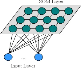
The neurons in the layer of an SOM are arranged originally in physical positions according to a specific topology such as grid, hexagonal, or random topology. A typical structure of SOM networks is shown in Fig. 1.
Fig. 1. A typical structure of SOM networks.
Training of SOM networks is based on Kohonen self-organization algorithm.
A SOM network identifies a winning neuron using the same procedure as employed by a competitive layer. However, instead of updating only the winning neuron, all neurons within a certain neighborhood Ni(d) of the winning neuron are updated, using the Kohonen rule. Specifically, all such neurons i
Ni(d) are adjusted as follows:( 1) ( ) [ ( ) ( )]
ij ij j ij
w k w k α v k w k (8)
where Wijis the weight of SOM layer from input i to neuron
j, vjis jth component of the input vector, α is learning rate
and k is discrete time.
Here the neighborhood Ni(d) contains the indices for all of the neurons that lie within a radius d of the winning neuron i. Thus, when an input vector is presented, the weights of the winning neuron and its close neighbors move toward the vector. Consequently, after many presentations, neighboring neurons have learned vectors similar to each other.
VII. DETAILS OF SELF-ORGANIZING NEURAL SYSTEM
Details of SONS and INS are similar. The main
difference between SONS and INS lies in their classifying unit. The details of SONS are explained as follows:
Firstly, the generated input-target training pairs are classified based on the natural periods of the structures. Input space classification is implemented by using a SOM neural network. Now it is possible to train an RBF network for each subspace using its training data. By considering the mentioned strategy, the single RBF network trained to cover all the input space is substituted with a set of some parallel RBF networks as each of them is trained to cover one specific part of the classified input space. A simple schema of SONS training flow is shown in Fig. 2.
Fig. 2. The flow of self-organizing RBF (SONS) training.
One of the most important difficulties of INS implementation is the determination of the number of data clusters. This difficulty is alleviated by using SOM neural network in the framework of SONS. In order to train the classifying unit of SONS a general grid of SOM neurons with random topology is considered. After training, the configuration of initial grid captures the shape of distribution of data in the input space. In this regard, the neurons tend to clustering and therefore the number of clusters can be simply determined mean of exact vectors component.
VIII. ERROR MONITORING
In order to evaluate the accuracy of approximate structural responses predicted by neural networks, two evaluation metrics are used: the relative root mean square (RRMS) error and R-square (R2) statistic measurement [14].
The RRMS error between the exact and predicted responses is defined as follows:
2 i i 1
r 2 i 1
1
( )
-1 RRMSE
1 ( )
r
i
i
r
r
(9)
To measure how successful fitting is achieved between exact and approximate time history responses, the R-square statistic measurement is employed. Statistically, the R2 is the square of the correlation between the predicted and the exact responses. It is defined as follows:
2 1
r
2 1
( )
- 1
( )
r
i i i
i i
R square
(10)
where,
is the mean of exact vectors component.IX. APPROXIMATION OF TIME HISTORY RESPONSES BY
SONS
The input space consists of some natural periods of the selected structures and the corresponding time history responses of nodal displacements and element internal stresses against earthquake are considered as the target space components. At first, a SOM network is trained to classify the input space based on the natural periods. To approximate time history responses of structures located in each subspace, a distinct RBF network is trained using the data located in it.
X. MAIN STEPS OF OPTIMIZATION
The fundamental steps in the optimization process by VSP using SONS for earthquake loading are as follows:
1) Selecting some parent vectors from the design variables space.
2) Evaluating the time history responses of the structure employing SONS.
3) Evaluating the objective function.
4) Checking the constraints at grid points for feasibility of parent vectors.
5) Generating offspring vectors using crossover and mutation operators.
6) Predicting the structural time history responses for the offspring population using trained SONS.
7) Evaluating the objective function.
8) Checking the constraints at grid points; if satisfied continue, else change the vector and go to step (f). 9) Checking convergence; if satisfied stop, else go to step
(e). - Selecting the majority parent vectors from the previous solution and some random design variables as a VSP.
Repeating steps (e) to (k) until the proper solution is met. As the size of populations in VSP is small the method is rapidly converged. It can be observed that during the optimization, the dynamic analysis of the structures is not needed. In fact, the necessary responses are found by the trained SONS.
XI. NUMERICAL EXAMPLE
One illustrative example is optimized for minimum weight. The time of optimization is computed in clock time by a personal Pentium IV 2000MHz. The earthquake records are applied in x direction. Young’s modulus is
2.1×10¹⁰ kg/m2, weight density is 7850 kg/m3. Cross-sectional area of the members are selected from the pipe, with radius to thickness less than 50, sections available in European profile list. The optimization is carried out by the VSP using following structural analysis methods:
1) Exact Analysis (EA).
2) Approximate analysis by a single RBF neural network (RBF).
TABLEI:SPECIFICATIONS OF VSPMETHOD
Population size 30
Crossover method One, two and three points crossover Crossover rate 0.9
Mutation rate 0.001 Maximum generation 15
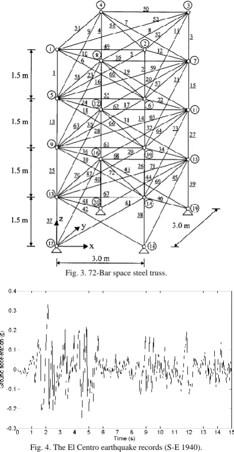
The 72-bar truss is shown in Fig. 3. The mass of 10000 kg is lumped at nodes of 1 to 4. The truss is subjected to 15 s of the earthquake record, shown in Fig. 4.
Fig. 3. 72-Bar space steel truss.
Fig. 4. The El Centro earthquake records (S-E 1940).
Due to simplicity and practical demands, the truss members are divided into 9 groups based on cross-sectional areas, shown in Table II.
TABLEII:ELEMENT GROUPS OF THE 72-BAR TRUSS
Group No. Elements
1 2 3 4 5 6 7 8 9
1-4 5-12 13-16 17-24 25-28 29-36 37-40 41-48 42-72
Because of the insignificant internal stresses of elements of group 9 under the earthquake excitation, a minimum cross-sectional area of 2.54 cm2 is assigned to them. For all the element groups, allowable stress is chosen to be 1200 kg/cm2. Also, for the top node of the structure, the allowable horizontal displacement is chosen to be 2 cm. In order to satisfy the practical demands, 8 types of cross-sectional areas are considered for the truss elements which are displayed in Table III.
TABLEIII:AVAILABLE CROSS-SECTIONAL AREAS
No. Area (cm2)
1 2 3 4 5 6 7 8
11.2 12.3 13.9 15.2 17.2 18.9 21.4 25.7
In the beginning, 300 structures are randomly generated based on cross-sectional areas and are subjected to the earthquake record. Their first, third and fifth natural periods are selected to be input space components. The corresponding node 1 displacement and axial stresses of element groups 1 to 8 are chosen as target space components. From which 220 and 80 samples are employed to train and to test the performance generality of the networks, respectively. A single RBF network is trained for predicting node 1 displacement and axial stress of each element groups. The first step in designing SONS is to classify the input space. At first, a 5×3×2 grid of SOM neurons with random topology is considered. After training the SOM networks, as shown in Fig. 5, it is observed that the neurons are grouped in three main clusters.
Fig. 5. Input data distribution on input space and a 5×3×2 grid of SOM neurons.
To eliminate redundant computations, a grid of 3×1×1 SOM neurons with random topology is adopted for this example. Thus, all the input data is divided into three clusters. Input data distribution and centre of clusters is shown in Fig. 6.
Fig. 6. Input data distribution on input space and centre of clusters.
The results of testing the single RBF and SONS neural networks are only shown for node 1 displacement and axial stress of group 7 elements in Figs. 7 to 10.
Fig. 7. 7: R-square of approximate displacement of node 1.
Fig. 8. RRMSE of approximate displacement of node 1.
Fig. 9. R-square of approximate stress of group 7 elements.
Fig. 10. RRMSE of approximate stress of group 7 elements.
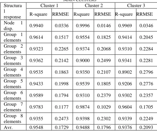
It is simple to find out from Figs. 7 to 10 that SONS possesses the better performance generality comparing with the single RBF network. The average R-square and RRMSE for single RBF and SONS for all training samples are 0.8956, 0.3207 and 0.9469, 0.1873, respectively. Mean R-square and mean RRMSE of predicted structural responses in all the clusters are displayed in Table IV. In this example, the total time spending to data generation and neural networks training is equal to 460 min.
solutions but it is very extensive in terms of the optimization over all time. Time history responses of optimum designs obtained using approximate analysis are compared with their corresponding actual ones. A brief summery is displayed in Table VI. The comparisons reveal the appropriate conformance between all of the approximate and corresponding actual responses. But the performance of SONS is better than that of the single RBF network.
TABLEIV:MEAN R-SQUARE AND RRMSE OF TEST DATA FOR THREE
MAIN CLUSTERS
Structura l response
Cluster 1 Cluster 2 Cluster 3
R-square RRMSE Rsquare RRMSE R-square RRMSE
Node 1
disp. 0.9940 0.0336 0.9996 0.0146 0.9969 0.0346 Group 1
elements 0.9614 0.1517 0.9554 0.1825 0.9414 0.2045 Group 2
elements 0.9323 0.2265 0.9374 0.2068 0.9310 0.2284 Group 3
elements 0.9362 0.2142 0.9000 0.2499 0.9341 0.2281 Group 4
elements 0.9535 0.1863 0.9350 0.2107 0.8902 0.2796 Group 5
elements 0.9433 0.1998 0.9539 0.1805 0.9206 0.2776 Group 6
elements 0.9589 0.1794 0.9310 0.2379 0.9302 0.2357 Group 7
elements 0.9783 0.1177 0.9874 0.1029 0.9604 0.1705 Group 8
elements 0.9355 0.2473 0.9398 0.2302 0.9339 0.2249 Avr. 0.9548 0.1729 0.9488 0.1796 0.9376 0.2093
TABLEV:OPTIMUM DESIGNS OBTAINED BY VSPUSING EXACT AND
APPROXIMATE ANALYSIS
Element Groups No. Optimum areas (cm
2)
EA RBF SONS
1 11.20 11.20 15.20
2 11.20 15.20 12.30
3 17.20 21.40 15.20
4 11.20 11.20 11.20
5 25.70 21.40 25.70
6 11.20 11.20 12.30
7 25.70 25.70 25.70
8 11.20 11.20 12.30
9 2.54 2.54 2.54
Weight (kg) 1506.60 1591.73 1586.79
Generations 57 62 60
Time (min) 2538.0 11.6 7.0
TABLEVI:MEAN R-SQUARE AND MEAN RRMSE OF OPTIMUM DESIGNS
Structural parameters SONS RBF
R-square RRMSE R-square RRMSE Node 1 displacement 0.9837 0.1277 0.9513 0.2206 Group 1 elements 0.9851 0.1223 0.8893 0.3327 Group 2 elements 0.9415 0.2419 0.8531 0.3832 Group 3 elements 0.9967 0.0576 0.7614 0.4885 Group 4 elements 0.9675 0.1973 0.9583 0.2041 Group 5 elements 0.9434 0.2379 0.8151 0.4300 Group 6 elements 0.9581 0.2046 0.9484 0.2272 Group 7 elements 0.9397 0.2235 0.9141 0.2856 Group 8 elements 0.9640 0.1897 0.9578 0.2053 Average. 0.9644 0.1781 0.8943 0.3086
The optimum design attained using SONS is better than that of the obtained using the single RBF network. It is important to note that, in this example the time of optimization employing neural networks, including data generation and training the neural networks is about 0.18 time of exact optimization.
XII. CONCLUSIONS
A robust optimization procedure has been developed for the optimal design of structures subjected to earthquake using discrete design variables. In the procedure, a combination of the evolutionary algorithm and neural networks has been utilized. The employed evolutionary algorithm is virtual sub population (VSP) method. The VSP method has eliminated the shortcomings of the standard GA such as trapping into local optima and much effort in the phase of computer implementation. Moreover, performing the structural optimization using the exact time history analysis for earthquake induced loads imposes a huge computational burden to the optimization process. That is, in each design point of the desired earthquake the structure should be analyzed to evaluate the necessary responses. To reduce the computer effort of the optimization process due to the performing time history analysis, a new neural system is employed. In the neural system, a specific combination of self-organizing map (SOM) and radial basis function (RBF) neural networks is employed to access high quality approximation of structural time history responses. The neural system is called self-organizing neural system (SONS). In fact, SONS includes two operational phases; classification and parallelization. In the classification phase the input space is classified employing a SOM neural network. In the parallelization phase, a distinct RBF neural network is trained for each class. In the present paper, RBF neural network and SONS is employed to approximate the necessary time history responses of structures. A simple method is employed to treat with dynamic constraints. In this method the time interval is divided into some subintervals and the constraints are imposed at each time grid points. The numerical results of optimization show that in the proposed methods, the time of optimization including training time is reduced to about 0.2 of the time required for exact optimization; however, the errors are small. Finally, it is demonstrated that the best solution has been attained by VSP method using SONS.
REFERENCES
[1] E. Salajegheh and A. Heidari, “Optimum design of structures against earthquake by wavelet neural network and filter banks,” Earthquake Engineering and Structural Dynamics, vol. 34, pp. 67–82, 2005. [2] S. Gholizadeh and E. Salajegheh, “An intelligent neural system for
predicting structural response subject to earthquakes,” in Proc. the Fifth International Conference on Engineering Computational Technology, 2006, p. 63.
[3] E. Salajegheh, J. Salajegheh, and S. Gholizadeh, “Structural optimization for earthquake loading using neural networks and genetic algorithms,” in Proc. the Eighth International Conference on Computational Structures Technology, 2006, p. 249.
[4] T. Kohonen, Self-Organization and Associative Memory, 2nd edition, Springer-Verlag, Berlin, 1987.
[5] ANSYS Incorporated, “ANSYS Release 8.1,” 2004.
[6] The Language of Technical Computing, MATLAB, Math Works Inc, 2004.
[7] E. Salajegheh and S. Gholizadeh, “Optimum design of structures by an improved genetic algorithm using neural networks,” Advances in Engineering Software, vol. 36, pp. 757-767, 2005.
[8] X. K. Zou and C. M. Chan, “An optimal resizing technique for seismic drift design of concrete buildings subjected to response spectrum and time history loadings,” Computers and Structures, vol. 83, pp. 1689-1704, 2005.
[10] J. D. Mathias, X. Balandraud, and M. Grediac, “Applying a genetic algorithm to the optimization of composite patches,” Computers and Structures, vol. 84, pp. 823-834, 2006.
[11] V. Govindaraj and J. V. Ramasamy, “Optimum detailed design of reinforced concrete continuous beams using genetic algorithms,”
Computers and Structures, vol. 84, pp. 34-48, 2005.
[12] G. A. Gazonas, D. S. Weile, R. Wildman, and A. Mohan, “Genetic algorithm optimization of phononic bandgap structures,”
International Journal of Solids and Structures, vol. 43, pp. 5851-5866, 2006.
[13] S. F. Hwang and R. S. He, “Improving real-parameter genetic algorithm with simulated annealing for engineering problems,”
Advances in Engineering Software, vol. 37, pp. 406-418, 2006.
[14] X. Jiang, S. Mahadevan, and H. Adeli, “Bayesian wavelet packet denoising for structural system identification,” Structural Control and Health Monitoring, 2006.
A. Lavaei is an academic member in the Department of Civil Engineering, College of engineering, Boroujerd Branch, Islamic Azad University, Iran. He started teaching civil course in Azad Islamic University since 2008.
His research interests are in optimization, genetic algorithm, earthquake, neural networks, and hazard assessment.