Development of Finite Difference Explicit and Implicit Numerical Reservoir Simulator for Modelling Single Phase Flow in Porous Media

(1)

Earth Sciences

2018; 7(6): 242-259

http://www.sciencepublishinggroup.com/j/earth doi: 10.11648/j.earth.20180706.11

ISSN: 2328-5974 (Print); ISSN: 2328-5982 (Online)

Development of Finite Difference Explicit and Implicit

Numerical Reservoir Simulator for Modelling Single Phase

Flow in Porous Media

Aphu Elvis Selase

1, *

, Brantson Eric Thompson

2

, Addo Bright Junior

3

, Akunda Doreen

4

1_{College of Public Administration, Huazhong University of Science and Technology, Wuhan, China} 2

School of Energy Resources, China University of Geosciences (Beijing), Beijing, China 3

Department of Economics and Geography & Resource Development, University of Ghana, Legon, Ghana 4_{College of Public Administration, Huazhong University of Science and Technology, Wuhan, China}

Email address:

*

Corresponding author

To cite this article:

Aphu Elvis Selase, Brantson Eric Thompson, Addo Bright Junior, Akunda Doreen. Development of Finite Difference Explicit and Implicit Numerical Reservoir Simulator for Modelling Single Phase Flow in Porous Media. Earth Sciences. Vol. 7, No. 6, 2018, pp. 242-259. doi: 10.11648/j.earth.20180706.11

Received: June 26, 2018; Accepted: October 4, 2018; Published: October 29, 2018

Abstract:

Every petroleum reservoir requires some means of predicting future performances as well as optimizing recovery of hydrocarbons under various operating conditions. Moreover, there is a need to simulate fluid flow in porous media due to the uncertainty and heterogeneity that is associated with petroleum reservoirs. Therefore, this study developed 1D finite difference explicit and implicit numerical reservoir simulator for modeling single phase flow in porous media. The explicit and implicit simulator developments consist of physical modeling, mathematical modeling, discretization of the models with finite difference scheme and transformation of the models into computer algorithms. Matlab codes were written to describe the fluid flow process to obtain the reservoir pressure distributions for each grid block at each timestep calculation. The explicit formulation linear equation was solved by the direct method while the implicit method was solved by the Jacobi iterative method. The numerical examples graphical plots generated from the simulator illustrate the average reservoir pressure depletion for the finite difference grid blocks. The plots for both the explicit and implicit method indicate decline in average reservoir pressure with time. The explicit and implicit simulators show that the implicit formulation is unconditionally stable than the explicit formulation. This is because the explicit method under certain conditions generates errors in the numerical solutions which tend to go zero during subsequent timestep calculations. Additionally, the porosity sensitivity analyses performed show that the average reservoir pressure decline as the porosity decreases from 30% to 10%. Material balance method was used to determine the average reservoir pressure decline for a one-year production period. The estimated recovery factor at the bubble point pressure is 0.68% of the original oil in place. This low recovery factor is a characteristic of an expansion-drive reservoir which has the least efficient recovery mechanism. Finally, the 1D explicit and implicit finite difference numerical simulators for predicting single phase flow reservoir pressure distributions during production periods are stepping stone towards implementing multiphase fluid flow formulations.

Keywords:

Explicit and Implicit Simulators, Material Balance Method, Jacobi Iterative Method, Explicit and Implicit Formulation, Numerical Simulator

1. Introduction

Reservoir simulation is the science of combining physics, mathematics, reservoir engineering, and computer

(2)

reservoir numerical simulators Zhangxin, 2007 [2]. The analogical methods utilize features of matured reservoirs that are analogous to the new target reservoirs in order to forecast production performance of these reservoirs. The experimental methods measure the physical properties such as saturation, pressure and flow rates in laboratory cores and then scale them up to the whole hydrocarbon accumulation. Additionally, the mathematical methods use model equations to forecast reservoir performance. The comprehensive details about these production forecasting methods can be found in the works of Ahmed 2006, [3] Chen et al. 2007 [4] Gates 2007 [5].

Reservoir simulation is a standard predictive engineering tool in the oil and gas industry used to obtain accurate well performance predictions for a hydrocarbon reservoir under different operating conditions. A hydrocarbon recovery project usually involves a huge capital investment of hundreds of millions of dollars, and the risk associated with its selected development and production strategies must be evaluated and minimized. These risks include such important factors as the complexity of a petroleum reservoir and the fluids filling it, the complexity of hydrocarbon recovery mechanisms, and the applicability of predictive methods. These complexities can be taken into account in reservoir simulation through data input into the simulation model, and this applicability can be estimated through sound engineering practices and accurate reservoir simulation. Therefore, this research involves the development of 1D numerical simulator using explicit and implicit finite difference numerical scheme for predicting pressure distribution in a production reservoir with the following objectives:

(1)To physically model single-phase fluid flow processes in the reservoir incorporating physics of the underlying physical phenomenon

(2)To derive a numerical model with the basic properties of both the physical and mathematical models

(3)To develop computer algorithms (Matlab programming codes) to solve efficiently the systems of linearized algebraic equations arising from the numerical discretization.

(4)To use the developed simulator to predict average reservoir pressure decline.

(5)To validate the developed simulator using the material balance method.

This research work is organized into five sections as follows: Section 2 describe the methodology for finite difference formulation. Section 3 describes the results and discussion from the ID explicit and implicit simulators developed. Finally, section 4 summarizes the conclusions drawn from this study. [6]

2. Methodology for Finite Difference

Formulation

The problem to be solved in reservoir modeling is to advance the simulation from the initial conditions to future times. This is accomplished by stepping through the simulation at discrete time intervals called timesteps. Two first order finite difference approximations of forward and backward difference formulations were employed to solve the pressure equations explicitly and implicitly. The discretization involves the process of converting the continuous equations into linear algebraic equations using finite difference method. Figure 1 below shows the discretization steps involved in the development of the numerical simulators.

Figure 1. Discretization Steps in the Development of the Numerical Reservoir Simulators Ertekin, 2007 [7].

Some of the advantages of the finite difference method as stated by Abbas Firoozabadi et al 2006 [8] include: simplicity, ease of extension from 1D to 2D and 3D, and also its compatibility with certain aspect of physics of two-and three-phase flow. However, it was pointed out that numerical dispersion and grid dependency are the two major disadvantages of this method. There are basically two types of finite-difference grids used in reservoir simulation: block-centered grid and point-distributed grid. In block-block-centered

grid, for a rectangular coordinate system, the grid block dimensions are selected first, followed by the placement of points in the central locations of the blocks. The distance between the block boundaries is the defining variable in space. In contrast, the grid points (or nodes) are selected first in the point-distributed grid Abou-Kassem et al., 2006 [9].

2.1. Linear Solvers in Reservoir Simulators

(3)

Earth Sciences 2018; 7(6): 242-259 244

greatest combined influence is the technique used to solve the large systems of equations arising from the numerical approximation of the nonlinear fluid flow equations. There are two general methods for solving the matrix equation resulting from the finite difference approximation, namely direct methods and iterative methods.

2.1.1. Direct Methods

These methods transform the original equations into equivalent equations that can be solved more easily. Popular direct solution methods include Gaussian elimination, Gauss-Jordan, and LU (Lower-Upper) decomposition. Ertekin et al. 2007 [7] stated that a direct solver has the capability to produce an exact solution after a fixed number of computations if the computer is able to carry an infinite number of digits. But, because all real computers have a finite word length, the solution obtained through a direct solver will have round-off errors. The direct solver is also limited by its excess computer storage requirements, since it is necessary that both the coefficient matrix and the right-hand vector throughout the solution process are to be stored

2.1.2. Iterative Solution Methods

The iterative process starts with an initial guess of the solution vector, and repeatedly refines the solution until a certain convergence criterion is reached. Popular iterative methods include the Jacobi iteration, Gauss-Siedel, successive over-relaxation (SOR), strongly implicit procedure (SIP), and conjugate-gradient method (CGM). But, in this study, the Jacobi iterative method was employed as the implicit equation solver. The iterative methods are generally slower than their direct counterparts due to the large number of iterations required. Also, the iterative methods do have significant computational advantages especially for large and sparsely populated coefficient matrix. However, Jaan 2006 [10] noted that the iterative methods do not always converge to the desired solution

2.2. Development of the Reservoir Numerical Simulator

The development of the 1D explicit and implicit numerical reservoir simulator include the under listed steps:

(1)Formulate the partial differential equations (PDE) of the model based on the oil reservoir characteristics, using the three basic laws governing fluid flow in porous media.

(2)Divide the reservoir into grids and then discretize the formulated partial differential equations in both space and time so as to obtain linearized system of equations. (3)Select an appropriate ordering scheme to obtain an

order of coefficients of the linear system of equations and then compute the pressure per grid block of the reservoir.

(4)Write codes for the system of equations using Matlab programming environment.

(5)Finally validate the numerical simulator using material balance method

2.3. Mathematical Model

The reservoir characteristics are expressed in term of the set of partial differential equations (PDEs) together with the appropriate initial and boundary conditions that approximate the fluid flow behaviour of the reservoir. There are basically three main laws which govern isothermal reservoir simulation:

(1)The law of mass conservation (2)Darcy’s law (transport equation), and

(3)Equation of state (Phase properties such as density, compressibility and formation volume factor).

2.4. Mathematical Model Description (Basic Assumption)

The mathematical model was developed under the following assumptions:

1 Homogeneous reservoir

2 Isothermal, single-phase and slightly compressible fluid 3 Steady state effective viscosity

4 Uniform grid size

5 Linear fluid flow into the wellbore 6 No-flow reservoir boundary condition 7 The fluid is Newtonian

8 Capillary and gravity forces are ignored. 9 The block-centered grid system was employed 10Chemical reactions are not included.

2.5. Basic Fluid Flow Equation

Considering the mass balance for a control volume, the mass conservation is given as:

(Total mass entering the CV during ∆t) − (Total mass leaving the CV during ∆t) = (Net change in mass within the CV during ∆t).

Since the equation constituting the mathematical model of the reservoir is too complex to be solved by analytical method, therefore, finite difference approximation is used to put the equation in a form that is amenable to solution by digital computer. The process involves spatial and time derivative discretization. The general PDE for a single phase three-dimensional flow through a porous medium may be written in Cartesian coordinates as expressed in Eq. (1) as:

β ∆x + β ∆y + β ∆z + q = (1)

From Eq. (1), a linear reservoir system is assumed in the x direction and the discretization is given by Eq. (2) as:

β

! !∆ "#$ %⁄ 'p"#$− p"* − β ! !∆ "+$ %⁄ 'p"− p"+$* + q,- "= . ∅0

! 12

"

34₍₂₎

(4)

T, "#$/%'p"#$− p"* − T, "+$/%'p"− p"+$* + q_{,- "}= . ∅0 ! 12

"

34₍₃₎

2.5.1. Forward-Difference Approximations for Fluid Flow Equation

The forward difference approximation for the flow equation at a base time level to the first derivative on the right-hand side of Eq. (3) is expressed in Eq. (4) as:

34_≈3489:+348

∆ (4)

Substituting Eq. (4) into Eq. (2) and (3) at time level tn results into Eq. (5) and (6) as:

β _{! !}_{∆ "#$/%}; 'p"#$; − p";* − β _{! !}_{∆ "+$/%} ;

'p";− p"+$; * + q,- "= . ∅_!1_∆02 "'p"

;#$_{− p}

"

;_*₍₅₎

In terms of transmissibilities,

T, "#$/%'p"#$; − p";* − T, "+$/%'p;" − p"+$; * + q,- "= . ∅_!1_∆02 "'p"

;#$_{− p}

"

;_*₍₆₎

2.5.2. Backward-Difference Approximations for Fluid Flow Equation

The backward-difference approximation generally is used in reservoir simulation because its use does not restrict the size of the timestep for stable solution. The backward difference approximation to the first derivative at the base time level is written in Eqs. (7) and (8) as:

3₌3<89:=+3'8*

∆ (7)

34_≈3489:+348

∆ (8)

Substituting into Eq. (8) at the time level tn+1 results into Eqs. (9) and (10) as:

β _{! !}_{∆ "#$/%}'p"#$;#$− p";#$* − β _{! !}_{∆ "+}: >

'p";#$− p"+$;#$* + q_{,- "}= . ∅_!1_∆02 "'p"

;#$_{− p}

"

;_*₍₉₎

T_{, "#$/%}'p"#$;#$− p";#$* − T_{, "+}: >'p"

;#$_{− p}

"+$ ;#$_{* + q}

,- "= . ∅_!1_∆02 "'p"

;#$_{− p}

"

;_*₍₁₀₎

3. Results and Discussion

Matlab is a high-level computer language for scientific computing and data visualization built around an interactive programming environment Ferreira, 2006. [11] The explicit and implicit codes developed in this paper were programmed in Matlab 2016 [12] environment. It is important to acknowledge here that all the numerical examples were taken

from Ertekin et al. 2007. [7]

3.1. Explicit Formulation Calculation Method

The forward difference approximation to the fluid flow equation results in an explicit calculation procedure for the new time level pressures. Solving the forward difference Eq. (6) for the unknown quantity, p_";#$, yields the expression in Eq. (11) as:

p";#$ = p";+ ! 1_∆

∅0 _"q,- "+ ! 1_∆

∅0 _"× @T, 49:/>

; _p

"#$

; _T

,;49:/>+ T,;4A:/> p;" + T,;4A:/>p"+$; B (11)

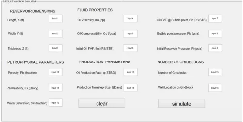
All the terms on the right hand side of Eq. (11) are known because all pressures appearing on this side are at the known (old) time level, n. In this equation, the pressures at the new time level can be obtained explicitly by the use of these known pressures. The Matlab code written for Eq. (11) is given in Appendix A. A graphical user interface (GUI) that accepts input data from the user was designed with Matlab for the explicit formulation finite difference simulator in this

(5)

Earth Sciences 2018; 7(6): 242-259 246

Figure 2. Explicit Numerical Reservoir Simulator Graphical User Interface.

3.2. Example Application of Explicit Scheme with Neumann Boundary Condition

For the 1D block-centered grids shown in Fig. 3 pressure distribution during the first year of production was determined. The initial reservoir pressure is 6000 psia. The rock and fluid properties for this problem are ∆x=1000 ft,

∆y=1000 ft, ∆z=75 ft, Bl=1 RB/STB, ct=3.5 x 10 -6

psi-1, kx=15 mD, ɸ=0.18, µl=10 cp, and B

o

l=1 RB/STB. Assuming

a timestep size of ∆t=10 days. Additionally, assuming that Bl

acts as a constant within the pressure range of interest and no flow boundary condition where the flux vanishes everywhere on the boundary.

Figure 3. Porous Medium and Block-Centered Grid System Ertekin et al., 2007 [7].

3.3. Explicit Simulation Results

Table 1 and Fig. 4 plots indicate the results that was generated from each timestep after running the simulator.

Table 1. Timestep Results of Explicit Simulator Calculations.

EXPLICIT SIMULATION STUDY RESULTS (∆t=10 DAYS) Time PRESSURE(PSIA)

(days) Block 1 Block 2 Block 3 Block 4 Block 5

0 6000.00 6000.00 6000.00 6000.00 6000.00

(6)

EXPLICIT SIMULATION STUDY RESULTS (∆t=10 DAYS) Time PRESSURE(PSIA)

20 6000.00 6000.00 5973.14 5697.21 5973.14

30 6000.00 5995.95 5935.61 5602.11 5931.56

40 5999.39 5987.47 5894.45 5523.75 5881.92

50 5997.59 5975.25 5852.61 5455.33 5827.95

60 5994.23 5960.14 5811.22 5393.09 5771.80

70 5989.09 5942.83 5770.66 5334.91 5714.74

80 5982.12 5923.86 5730.94 5279.55 5657.50

90 5973.34 5903.57 5691.99 5226.26 5600.55

100 5962.83 5882.20 5653.70 5174.59 5544.15

110 5950.68 5859.92 5615.93 5124.21 5488.46

120 5937.00 5836.83 5578.60 5074.94 5433.58

130 5921.91 5813.01 5541.62 5026.62 5379.54

140 5905.50 5788.53 5504.91 4979.15 5326.36

150 5887.87 5763.42 5468.42 4932.44 5274.04

160 5869.12 5737.72 5432.11 4886.42 5222.56

170 5849.32 5711.47 5395.93 4841.05 5171.91

180 5828.55 5684.70 5359.87 4796.26 5122.06

190 5806.87 5657.43 5323.89 4752.03 5072.96

200 5784.35 5629.69 5287.98 4708.30 5024.60

210 5761.05 5601.50 5252.12 4665.06 4976.94

220 5737.01 5572.90 5216.30 4622.26 4929.95

230 5712.28 5543.89 5180.52 4579.88 4883.58

240 5686.90 5514.51 5144.77 4537.90 4837.82

250 5660.93 5484.77 5109.04 4496.28 4792.63

260 5634.38 5454.70 5073.32 4455.02 4747.97

270 5607.31 5424.31 5037.62 4414.08 4703.83

280 5579.73 5393.62 5001.93 4373.44 4660.17

290 5551.69 5362.64 4966.25 4333.10 4616.96

300 5523.20 5331.40 4930.57 4293.02 4574.19

310 5494.30 5299.90 4894.90 4253.20 4531.82

320 5465.01 5268.17 4859.23 4213.63 4489.84

330 5435.35 5236.21 4823.57 4174.28 4448.22

340 5405.34 5204.04 4787.91 4135.14 4406.94

350 5375.01 5171.67 4752.25 4096.20 4365.98

(7)

Earth Sciences 2018; 7(6): 242-259 248

Figure 4. Explicit Pressure against Time Plot for Gridblocks.

3.4. Discussion of Explicit Simulation Results

The first point is that no-flow boundary conditions can be modeled by assigning zero transmissibility at the edges of the porous medium. The second point is that the pressures calculated at identical times are different, depending on the timestep size used in the calculation as shown in Table 1. This is indicative of the approximate nature of the finite difference technique. There is no reason why these approximations should give the same result for different timestep sizes. Because the approximation is first order, the smaller timestep sizes generally give more precise results when compared with the solution of the original PDE. Another point illustrated by this example is that the pressure transient created by fluid withdrawal from the well in Gridblock 4 can only move one cell per timestep as shown in Table 1. This is a property of the explicit method only. For a timestep size of 10 days, it takes the pressure transient 40 days to reach the left boundary, while for a timestep size of 30 days; it would have taken the pressure transient 120 days to reach the boundary. That is, four timesteps are always needed for the pressure transient to reach the left boundary in this example calculation (Table 1). The difference that will occur when a constant pressure (pressure-specified boundary) is specified at either side of the gridblock is that the pressure distribution at the end of the first year of production (360 days) in the gridblock containing the well will be greater than the case of no-flow boundary condition. This is because the pressure that will be specified at either boundary of the gridblock provides support to the gridblock containing the well. This type of boundary condition occurs in a reservoir that is constantly charged by strong water influx, so that the pressure at the interface between the hydrocarbon reservoir and the supporting aquifer remains constant which is known as Dirichlet problem). The method of implementing the specified boundary pressure is the least rigorous method available for block centered grid systems. This is because the

pressure on the boundary is shifted from the gridblock edge to the block center (i.e ∆x/2 away from the reservoir boundary). Although, this method is the least accurate method of implementing boundaries with specified pressure, it is the most practical method of implementation. As a result, it is the most common method of implementing boundaries with specified pressure in reservoir simulators. One method to improve the description of a constant-pressure boundary is to use a more refined grid in the vicinity of the pressure-specified boundary. In general, this method can improve the accuracy of modeling boundaries with specified pressure in block-centered grids. For the explicit solution technique, this may lead to stability problems. This erratic behavior is caused by the conditional stability nature of the explicit forward difference scheme formulation. The forward difference equation is conditionally stable, because under certain conditions, the errors in the solution tend to go to zero during the subsequent timestep calculations. Meanwhile, under other conditions, these same errors propagate uncontrollably during subsequent timestep calculations. This is a serious limitation of the forward difference formulation. In summary, the implementation of the explicit formulation technique involves pressures at the old-time-level only. At this time level, these quantities are known and can be used in an explicit calculation procedure to advance the simulation in time.

3.5. Discussion of Analytical Results

All that is necessary is to devise some means of averaging individual well pressure declines to determine a uniform trend for the reservoir as a whole. The average pressure decline can be determined by the volume weighting of pressures within the drainage area of the well. If pj and Vj

(8)

PD =∑ 3F F F

∑F F (12)

The obtained average reservoir pressure using Eq. (12) for an explicit numerical computation is given as:

PD = 4846.753806 psia

Material balance method in Eq. (13) was used to find the total cumulative oil production for a one year production period using the explicit numerical simulator results as:

q RS

(13)

Np=150x360 =54,000 STB

Furthermore, the recovery factor at the bubble point pressure is computed using Eq. (14) as:

R RS

RU 4C ∆P (14)

R 1_{1 ? 3.5 ? 10}+X_{? '6000 ) 4,057.40*}

R=0.0067991

The estimated recovery factor at the bubble point pressure is 0.0067991 of the original oil in place. This low recovery factor is a characteristic of an expansion-drive reservoir which has the least efficient recovery mechanism Dake, 1998 [13]; Fanchi, 2008 [14]; Tarek, 2006 [15]. A sensitivity study was also conducted on the simulator developed to observe the effect of porosity on average reservoir pressure as shown in Fig. 5. The sensitivity analysis performed to investigate the effect of porosity on average reservoir pressure shows that the average reservoir pressure decline as the porosity decreases from 30% to 10%. This indicates that the time taken to reach the bubble point pressure decreases as the porosity decreases.

Figure 5. Effect of porosity on average reservoir pressure.

3.6. Implicit Calculation Method

The backward difference approximation to the slightly compressible flow equation results in an implicit calculation procedure for the new-time-level pressures. Rearranging Eq. (10) yields Eq. (15) as:

T_{, "#$/%}p"#$;#$) Z. ∅_!1_∆02

" T, "#:> T, "+:>[ p"

;#$ _T

, "+: >? p"+$

;#$ _{) Zq}

,- " . ∅_!1_∆02 "p"

;_[₍₁₅₎

where the quantities p_"#$;#$ , p_";#$and p_"+$;#$ are all unknowns. Unlike the explicit formulation, Eq. (15) cannot be solved explicitly for p_";#$ because both p_"#$;#$ and p_"+$;#$ are also unknown. As a result, Eq. (15) written for all gridblocks and

(9)

Earth Sciences 2018; 7(6): 242-259 250

Figure 6. Implicit Simulator Graphical User Interface.

3.6.1. Example Application of Neumann Boundary Condition

The same problem described for the explicit method was used for the implicit backward difference formulation. Herein, assuming a timestep size of ∆t = 15 days

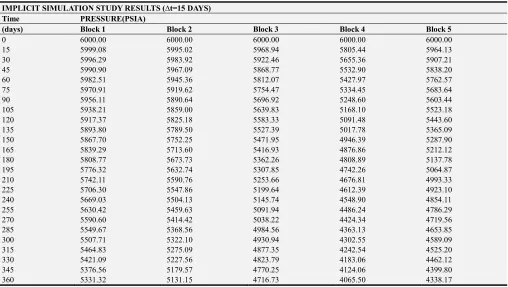
3.6.2. Implicit Simulation Results

Table 2. Implicit Simulation Pressure Results.

IMPLICIT SIMULATION STUDY RESULTS (∆t=15 DAYS)

Time PRESSURE(PSIA)

0 6000.00 6000.00 6000.00 6000.00 6000.00

15 5999.08 5995.02 5968.94 5805.44 5964.13

30 5996.29 5983.92 5922.46 5655.36 5907.21

45 5990.90 5967.09 5868.77 5532.90 5838.20

60 5982.51 5945.36 5812.07 5427.97 5762.57

75 5970.91 5919.62 5754.47 5334.45 5683.64

90 5956.11 5890.64 5696.92 5248.60 5603.44

105 5938.21 5859.00 5639.83 5168.10 5523.18

120 5917.37 5825.18 5583.33 5091.48 5443.60

135 5893.80 5789.50 5527.39 5017.78 5365.09

150 5867.70 5752.25 5471.95 4946.39 5287.90

165 5839.29 5713.60 5416.93 4876.86 5212.12

180 5808.77 5673.73 5362.26 4808.89 5137.78

195 5776.32 5632.74 5307.85 4742.26 5064.87

210 5742.11 5590.76 5253.66 4676.81 4993.33

225 5706.30 5547.86 5199.64 4612.39 4923.10

240 5669.03 5504.13 5145.74 4548.90 4854.11

255 5630.42 5459.63 5091.94 4486.24 4786.29

270 5590.60 5414.42 5038.22 4424.34 4719.56

285 5549.67 5368.56 4984.56 4363.13 4653.85

300 5507.71 5322.10 4930.94 4302.55 4589.09

315 5464.83 5275.09 4877.35 4242.54 4525.20

330 5421.09 5227.56 4823.79 4183.06 4462.12

345 5376.56 5179.57 4770.25 4124.06 4399.80

(10)

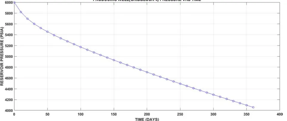
Figure 7. Implicit Pressure against Time Plot for Gridblocks.

3.6.3. Discussion of Implicit Simulation Results

The example calculation illustrates that the amount of computation required for the implicit solution procedure is much greater than that for the explicit solution procedure. This is because, at each timestep, a system of equations must be solved for the unknowns of the problem. In general, most of the computational time used in implicit simulation is in the solution of the linear equation. This example also illustrates that the reservoir pressure can move more than one gridblock per timestep as shown in Table 2. Herein, it has moved to the left boundary during the first timestep. Also, the results from the implicit backward difference formulation and the explicit forward difference formulation will not give identical results even when the same timestep is used. This is because of the approximate nature of the finite difference approach. Moreover, the no-flow boundary can be implemented by assigning zero transmissibility to the boundaries. This

example also demonstrates that no stability problem is associated with the implicit formulation. This is because the implicit formulation is unconditionally stable. This property states that no conditions exist where the backward difference formulation exhibits unstable behavior. Although this statement indicates that any gridblock dimension and /or timestep size can be used with no stability problems, the use of large timestep sizes and block dimensions may result in unrealistic coarse approximations. This becomes apparent in the solution as a departure from the true physics of the problem. However, due to the unconditionally stable nature of the implicit formulation, the backward difference formulation is the most commonly used formulation in petroleum reservoir simulation Ertekin et al. 2007. [7]

4. Conclusions

(11)

Earth Sciences 2018; 7(6): 242-259 252

of implementing boundaries with specified pressure, it is the most practical method of implementation. Thus, it is the most common method of implementing boundaries with specified pressure in numerical reservoir simulators.

On the other hand, the implicit formulation method also demonstrates that no stability problem is encountered as compared to explicit formulation. This is because the implicit formulation is unconditionally stable. Material balance method was also employed to validate the reservoir simulator that was developed. Additionally, the 1D explicit and implicit finite difference numerical simulator developed for predicting single phase pressure distributions in a reservoir during production is a stepping stone towards implementing two or three phase multiphase flow

Numerical methods such as finite element method, integral volume, finite volume method, and variational method could

be employed for the discretization of the PDE governing the fluid flow process and compared to the finite difference method used in this study. This will accommodate both regular and irregular reservoir geometry. In the implicit method implemented in this study, it was observed that the number of iterations required for convergence was large. This may be significantly reduced by introducing preconditioners used to reduce the matrix condition number and speed up the convergence of iterative solvers in order to increase the convergence rate.

Acknowledgements

Thanks to the anonymous reviewers for their comments and suggestions that were instrumental in improving the manuscript.

Appendix

Appendix A: Matlab Code for Explicit Calculation Procedure

clear all; close all; clc; clf

% ========================================================================== %PROBLEM FORMULATION

%Explicit Finite Difference Formulation %1D block centered grid

%Determine the pressure distribution during first year of oil production

========================================================================== %POROUS MEDIUM AND BLOCK CENTERED GRID SYSTEM

%

% ^ qsc=-150STB/D % |

% |---|---|---|--- |---|

% | | | | | | | % 75ft | o | o | o | o | o |

% | | | | | |

% | 1 | 2 | 3 | 4 | 5 | % |---|---|---|---|---| % dp/dx=0 1000ft dp/dx=0

%CREATE INPUT VALUES FOR RESERVOIR PROPERTIES x=input('Enter change in x length value:');

y=input('Enter change in y length value:'); z=input('Enter change in z length value:'); Bo=input('Enter initial formation volume factor:'); Bl=input('Enter liquid phase formation volume factor:'); ct=input('Enter compressibility factor:');

(12)

%CALCULATE EXPLICIT FORMULAR PROPERTIES a=y*z; %Calculate the area of gridblocks.unit: ft2

vb=x*y*z; %Calculate the volume of gridblocks.unit: ft3 alpha=(5.615*Bl*t)/(vb*o*ct); %Calculate explicit factor

beta=(1.127*a*k)/(ul*Bl*x); %Calculate the transmissibility of gridblocks ksi=beta;

%SETTING INITIAL CONDITIONS P0=0; %For block one Pi-1=P0=1, where i=1

P=ones(1,5)*Pi; %Pi=6000psia for Gridblocks i=1,2,3,4,5

%LOOPING TO CALCULATE TIMESTEP %tstep=timestep

for tstep=1:5 for block = 1:5

%BOUNDARY CONDITIONS FOR GRIDBLOCKS

alpha(1,block)=(5.615*Bl*t)/(vb*o*ct) if block==1

ksi(1,block)=0 else

ksi(1,block)=(1.127*a*k)/(ul*Bl*x) end

if block~=4 q(1,block)=0 else

q(1,block)=-150 end

if block==5 beta(1,block)=0 else

beta(1,block)=(1.127*a*k)/(ul*Bl*x) end

gamma=beta+ksi;

%CALCULATION OF PRESSURE DISTRIBUTION IN BLOCKS AT EVERY TIMESTEP if block ~=5

if block ==1

P(tstep + 1,block) = P(tstep,block)+ alpha(1,block)*q(1,block) +alpha(1,block)*(beta(1,block) *P(tstep,block+1)- ... gamma(1,block)*P(tstep ,block) + ksi(1,block)*P0)

else

P(tstep + 1,block) = P(tstep,block)+ alpha(1,block)*q(1,block) +alpha(1,block)*(beta(1,block)*P(tstep,block+1) - gamma(1,block)*P(tstep ,block) +ksi(1,block)*P(tstep ,block-1))

end

elseif block==5

P(tstep + 1,block) = P(tstep,block)+ alpha(1,block)*q(1,block) +alpha(1,block)*(beta(1,block)*P(tstep,block) - gamma(1,block)*P(tstep ,block) + ksi(1,block)*P(tstep ,block-1))

end end end

%PLOTTING RESULTS figure(1)

x=(0:10:360)'; y=P(:,1);

subplot(2,2,1); % defining 1st plotting area plot(x,y,'-bo')

(13)

Earth Sciences 2018; 7(6): 242-259 254

title('PRODUCING WELL(GRIDBLOCK 1) PRESSURE VRS TIME'); xlabel('TIME (DAYS)');

ylabel('RESERVOIR PRESSURE (PSIA)'); grid on

x=(0:10:360)'; y=P(:,2);

box on;

x=(0:10:360)'; y=P(:,3);

box on;

x=(0:10:360)'; y=P(:,5);

box on;

figure(2) x=(0:10:360)'; y=P(:,4); plot(x,y,'-bo') box on;

Appendix B: Matlab Code for Implicit Calculation Procedure

clear all; close all; clc; clf

========================================================================== %PROBLEM FORMULATION

%Explicit Finite Difference Formulation %1D block centered grid

%Determine the pressure distribution during first year of oil production

(14)

% ^ qsc=-150STB/D % |

% |---|---|---|--- |---|

% | | | | | | | % 75ft | o | o | o | o | o |

% | | | | | |

% | 1 | 2 | 3 | 4 | 5 | % |---|---|---|---|---| % dp/dx=0 1000ft dp/dx=0

%CREATE INPUT VALUES FOR RESERVOIR PROPERTIES x=input('Enter change in x length value:');

y=input('Enter change in y length value:'); z=input('Enter change in z length value:'); Bo=input('Enter initial formation volume factor:'); Bl=input('Enter liquid phase formation volume factor:'); ct=input('Enter compressibility factor:');

k=input('Enter permeability value:'); ul=input('Enter viscosity value:'); o=input('Enter porosity value:'); t=input('Enter timestep sizes:'); q=input('Enter reservoir flowrate:'); Pi=input('Enter initial pressure');

%CALCULATE EXPLICIT FORMULAR PROPERTIES a=y*z; %Calculate the area of gridblocks.unit: ft2

vb=x*y*z; %Calculate the volume of gridblocks.unit: ft3 alpha=(5.615*Bl*t)/(vb*o*ct); %Calculate explicit factor

beta=(1.127*a*k)/(ul*Bl*x); %Calculate the transmissibility of gridblocks ksi=beta;

%CALCULATION OF PARAMETERS Ax=y*z

Vb=x*y*z

T=(beta_c*Ax*kx)/(ul*Bl*x); rows = 5;

cols = 5; P = zeros(24,5); P =ones(1,5)*6000;

Mat_of_Coeff = zeros(rows,cols); Rhs = zeros(5,1);

coeff = 1; for block = 1:5

G(1,block) = (Vb*phi*ct)/(alpha_c*Bl*t)

if block==1 ksi(1,block)=0 else

ksi(1,block)=0.1268 end

if block~=4 q(1,block)=0 else

(15)

Earth Sciences 2018; 7(6): 242-259 256

if block==5 beta(1,block)=0 else

beta(1,block)=0.1268 end

gamma=beta+ksi if(block == 1)

Mat_of_Coeff(block, coeff+1) = beta(1,block)

Mat_of_Coeff(block, coeff) = - G(1,block) - gamma(1,block) Mat_of_Coeff(block, coeff+2) = ksi(1,block)

elseif(block ==2)

Mat_of_Coeff(block, coeff) = beta(1,block)

Mat_of_Coeff(block, coeff+1) = - G(1,block) - gamma(1,block) Mat_of_Coeff(block, coeff+2) = ksi(1,block)

elseif(block>2 && block <5)

Mat_of_Coeff(block, block-1) = beta(1,block)

Mat_of_Coeff(block, block) = - G(1,block) - gamma(1,block) Mat_of_Coeff(block, block+1) = ksi(1,block)

elseif(block ==5)

Mat_of_Coeff(block, block-2) = beta(1,block)

Mat_of_Coeff(block, block) = - G(1,block) - gamma(1,block) Mat_of_Coeff(block, block-1) = ksi(1,block)

end end

for tstep= 1:24 if(tstep ==1) for block = 1:5

Rhs(block) = -(q(1,block) +Pi*G(1,block)) end

P1 = (Mat_of_Coeff\Rhs)' for(block =1:5)

P(tstep+1,block) = P1(block) end

elseif(tstep >=2 && tstep<=24) for block = 1:5

Rhs(block) = -(q(1,block) +P1(block)*G(1,block)) end

P1 = (Mat_of_Coeff\Rhs)' for(block =1:5)

P(tstep+1,block) = P1(block) end

end

JACOBI ITERATIVE SOLUTION METHOD A=Mat_of_Coeff

b= Rhs

% Set initial value of x to zero column vector x0=zeros(1,5)

% Set Maximum iteration number k_max k_max=1000;

% Set the convergence control parameter erp erp=0.0001;

(16)

for i=1:5 s=0.0 for j=1:5 if j==i continue else

s=s+A(i,j)*x0(j) end

end

x1(i)=(b(i)-s)/A(i,i) end

if norm(x1-x0)<erp break

else x0=x1 end end

% show the final solution x=x1'

% show the total iteration number n_iteration=k

for(block =1:5)

P(tstep+1,block) = x(block) end

end end

%PLOTTING RESULTS figure(1)

x=(0:15:360)'; y=P(:,1);

box on;

x=(0:15:360)'; y=P(:,2);

box on;

x=(0:15:360)'; y=P(:,3);

box on;

(17)

Earth Sciences 2018; 7(6): 242-259 258

x=(0:15:360)'; y=P(:,5);

box on;

figure(2) x=(0:15:360)'; y=P(:,4); plot(x,y,'-bo') box on;

NOMENCLATURE

A = Cross-sectional area normal in the direction of flow, (ft2) Bo = Oil formation volume factor (rb⁄stb)

βC = Unit conversion factor for the permeability coefficient = 1.127, ∆t = Time step (day)

∆x = \]^_`ℎbcd_efghibjk (c`) ∆y = lfg`ℎbcd_efghibjk (c`) ∆z = m]f_ℎ`bcd_efghibjk (c`) µ = Oil viscosity (cp)

Gi,j,k = Constant part of the transmissibility, (stb/day-psi) H = Formation thickness (ft)

K = Rock permeability (d)

Kx = Formation permeability in x-direction (d or md) Ky = Formation permeability in y-direction (d or md) Kz = Formation permeability in z-direction (d or md) Lx = Formation length in x-direction (ft)

Ly = Formation length in y-direction (ft) ɸ = formation porosity (fraction) P = Reservoir pressure (psia)

q = Volumetric flow rate of production (stb⁄D) qi,j,k = Oil flow rate from well in cell i,j,k (stb/day) t = Time step (day)

T = Transmissibility, (stb/day-psi)

Ti,j,k+1/2 = Transmissibility along z-direction between cell (i,j,k) and cell (i,j,k+1/2), (stb/d-psi) Ti,j+1/2,k = Transmissibility along y-direction between cell (i,j,k) and cell (i,j+1/2,k), (stb/d-psi) Ti+1/2,j,k = Transmissibility along x-direction between cell (i,j,k) and cell (i+1/2,j,k), (stb/d-psi) Vb = Volume at reservoir condition (rb)

x = x-direction y = y-direction z = z-direction

nx = total number of grid cells in the x-direction ny = total number of grid cells in the y-direction nz = total number of grid cells in the z-direction Z = Elevation (ft)

(18)

γ = Fluid gravity (psi⁄ft)

ρ = Density at reservoir condition o = Oil

n = Previous time step n+1 = Next time step

References

[1] Aziz, K. and Settari, A., Petroleum Reservoir Simulation, Applied Science Publishers, 1979.

[2] Zhangxin Chen, Mathematical Techniques in Oil Recovery, SIAM, 2007.

[3] T. Ahmed (2006), Reservoir Engineering Handbook, Society of Petroleum Engineers, Richardson, TX.

[4] Z. Chen, J. Adams, D. Carruthers, H. Chen, I. Gates, G. Huan, S. Larter, W. Li, and G. Zhou (2007b), Coupled reservoir simulation and basin models: Reservoir charging and fluid mixing, to appear.

[5] I. Gates (2007), Basic Reservoir Engineering, in progress. [6] The MathWorks, Inc., MATLAB: The Language of Technical

[7] Ertekin, T., Abou-Kassem, J. H., and King, G. R., Basic Applied Reservoir Simulation, SPE Textbook Volume 10, 2007.

[8] Abbas, F., Thermodynamics of Hydrocarbon Reservoirs, McGraw-Hill, 2006.

[9] Abou-Kassem, J. H., Farouq Ali, S. M., and Islam, M. R., Petroleum Reservoir Simulation: A Basic Approach, Gulf Publishing Company, Houston, TX, USA, 2006.

[10] Jaan Kiusalaas, Numerical methods in engineering with Matlab®. The Pennsylvania State University, Cambridge University press, New York, 2006.

[11] Ferreira, A. J. M. (2009). MATLAB Codes for Finite Element Analysis. Springer. ISBN 978-1-4020-9199-5.

[12] Brian R. Hunt, Ronald L. Lipsman and Jonathan M. Rosenberg, A Guide to MATLAB®: for Beginners and Experienced Users: Third Edition, 2014.

[13] Dake, L. P., Fundamentals of Reservoir Engineering, Elsevier, Amsterdam, Netherlands, 2010.

[14] Fanchi, J. R., Principles of Applied Reservoir Simulation, Houston, Tex, Gulf Pub, 2008.