An Effect of Background Population Sample Size on the Performance of
a Likelihood Ratio-based Forensic Text Comparison System:
A Monte Carlo Simulation with Gaussian Mixture Model
Shunichi Ishihara
Department of Linguistics, The Australian National University
Abstract
This is a Monte Carlo simulation-based study that explores the effect of the sample size of the background database on a likelihood ratio (LR)-based forensic text comparison (FTC) system built on multivariate authorship attrib-ution features. The text messages written by 240 authors who were randomly selected from an archive of chatlog messages were used in this study. The strength of evidence (= LR) was estimated using the multivariate kernel density likelihood ratio (MVKD) formula with a logistic-regression calibration. The results are reported along two points: the system formance (= accuracy) and the stability of per-formance based on the standard metric for LR-based systems; namely the log-likelihood-ratio cost (Cllr). It was found in this study that the system performance and its stability im-prove as a function of the sample size (= au-thor count) in the background database in a non-linear manner, and that the more features used for modelling, the more background data the system generally requires for optimal re-sults. The implications of the findings to the real casework are also discussed.
1 Introduction
1.1 Forensic text comparison and the likeli-hood-ratio framework
The conceptual framework of likelihood ratio (LR) has received or has started receiving wide support from various areas of forensic comparative scienc-es as the logically and legally correct framework for assessing forensic evidence, and presenting the strength of the evidence (Balding, 2005; Evett et al., 1998; Marquis et al., 2011; Morrison, 2009; Neumann et al., 2007). Although forensic text
comparison (FTC) is lagging behind other areas of forensic comparative sciences, studies in which the LR framework was applied to authorship attribu-tion have started emerging (Ishihara, 2012, 2014b).
As expressed in equation (1), the LR, the quanti-fied strength of evidence, is a ratio of two condi-tional probabilities: one is the probability (p) of observed evidence (E) assuming that the prosecu-tion hypothesis is true (Hp) and the other is the
probability of the same observed evidence assum-ing that the defence hypothesis (Hd) is true
(Robertson & Vignaux, 1995).
For FTC, for instance, it will be the probability of observing the difference (referred to as the evi-dence, E) between the offender’s and the suspect’s text messages if they had been produced by the same author (Hp) relative to the probability of
ob-serving the same evidence (E) if they had come from different authors (Hd).
In practice, an LR is estimated as a ratio of two terms: similarity and typicality, which correspond to the numerator and denominator of equation (1). Similarity means the similarity (or difference) be-tween the offender and the suspect samples (e.g. text messages). Typicality means, in general terms, the typicality (or atypicality) of the offender sam-ple against the relevant population. If the offender and the suspect samples are more similar or more atypical, the LRs will be greater than when the same samples are more different or more typical.
It is important to emphasise that for example, LR = 100 does not mean that it is 100 times more likely that the offender and the suspect are the same person, but it means that the evidence is 100 times more likely to arise if the offender and the s-
LR=p(E|Hp)
uspect samples had been produced by the same individual, than by differ-ent individuals.
As can be well under-stood from the concept of typicality, besides the offender and the suspect samples, it is an essential part of the LR framework to have samples from a relevant population for
typicality. It goes without saying that an appropri-ate amount of data is required as relevant popula-tion data (= background data) to build an accurate model for typicality. Yet, how much do we need?
1.2 Research question
Having briefly outlined the key concepts of the LR framework, the present study investigates how the sample size of the background data influences the performance of the LR-based FTC system.
For this, a series of experiments was repeatedly carried out with the synthetic background data generated by the Monte Carlo technique, which are different in sample size (= different numbers of authors). The performance of the FTC system was assessed by the log likelihood ratio cost (Cllr)
(Brümmer & du Preez, 2006). Three different lengths: 500, 1000 and 1500 words and four fea-ture vectors: two, four, six and eight feafea-tures were used in the experiments to see how these factors also contribute to the performance.
1.3 Previous studies
It can be considered that the greater the amount of representative data, the more accurate the model of the reference population, leading to a more accu-rate estimate of strength of evidence. A small number of studies have investigated the effect of sample size in the background database on the sys-tem performance, in particular, in the field of fo-rensic voice comparison (Hughes et al., 2013; Ishihara & Kinoshita, 2008), and reported a similar outcome that the performance of a system becomes stable with greater than 20 reference individuals. However, those studies are voice/speech as evi-dence and did not consider the number of features in vectors.
2 Research Design
2.1 Database
An archive of chatlog messages1, which is a collec-tion of real pieces of chatlog evidence used to prosecute paedophiles, was employed in this study. From the archive, 240 authors were randomly se-lected. Two non-overlapping fragments (in other words, two message groups) of 500 words were extracted from each author’s messages so that one fragment can represent the offender and the other the suspect. The same was repeated for 1000 and 1500 words. As a result, there are altogether 480 message groups (= 240 authors × 2 message groups). The chatlog messages were tokenised into word tokens using WhitespaceTokenizer() stored in the Natural Language Tool Kit (NLTK) (version 2.0)2.
The 240 authors were further divided into mutu-ally-exclusive test (50 authors), background (140 authors) and development (50 authors) databases. The test database is used to assess the performance of the FTC system by comparing the message groups with the derived LRs. A more detailed ex-planation for testing is given in §2.4. The back-ground database is used as the reference database (in terms of typicality) for calculating LRs. The development database is to calculate weights for calibrating the derived LRs from the test database. §2.5 explains calibrations in detail.
2.2 Features
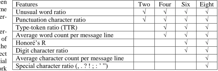
In this study, the four different feature vectors giv-en in Table 1 were used for modelling each mes-sage group. These four vectors consist of either two, four, six or eight features. These were
1 http://pjfi.org/
2 http://www.nltk.org/
Features Two Four Six Eight
Unusual word ratio √ √ √ √
Punctuation character ratio √ √ √ √
Type-token ratio (TTR) √ √ √
Average word count per message line √ √ √
Honoré’s R √ √
Digit character ratio √ √
Average character count per message line √
[image:2.595.172.532.109.227.2]Special character ratio (, . ? ! ; : ’ ”) √
ed from 11 features, which were previously report-ed as carrying good authorial information (De Vel et al., 2001; Iqbal et al., 2010; Zheng et al., 2006). They are: 1) Yule’s I (the inverse of Yule’s K), 2) Type-token ratio (TTR), 3) Honoré’s R, 4) Aver-age word count per messAver-age line, 5) Unusual word ratio, 6) Average character count per message line, 7) Upper case character ratio, 8) Digit character ratio, 9) Average character count per word, 10) Punctuation character ratio and 11) Special charac-ter ratio (, . ? ! ; : ’ ”). Based on these, a series of FTC experiments was carried out with all possible combinations of two, four, six and eight features in order to identify which combinations perform best. The combinations listed in Table 1 returned the
best Cllr values, respectively for the sets of two,
four, six and eight features.
Many of the features given in Table 1 are self-explanatory. The unusual_words() function3 of the
NLTK was used to obtain “Unusual word ratio” (e.g. unusual and misspelt words). TTR and Honoré’s R are so-called vocabulary richness fea-tures.
2.3 Repeated experiments using Monte Carlo techniques
If the current study had been conducted with natu-ral data, sufficiently large amounts of text
[image:3.595.101.495.102.497.2]
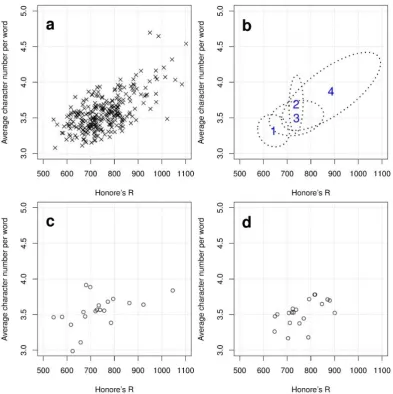
es written by a substantial number of authors would have been required. However, due to a lack of such a database of extensively large natural da-ta, the Monte Carlo simulations were employed for this study (Fishman, 1995). The Monte Carlo simulations enable us to generate synthetic values from the specified statistical properties of a distri-bution. It is common to use a single Gaussian component to model a distribution in the Monte Carlo simulations. However, the Gaussian mixture model (number of components = 4) was utilised in this study. This is because the distributional pat-terns of the features concerned in the current study do not always conform to a normal distribution as can be seen in Panel a of Figure 1, in which the sampled values of ‘Honoré’s R’ and ‘Average character count per message line’ are plotted.
The process of the Monte Carlo simulation is il-lustrated in Figure 1, using the feature values of ‘Honoré’s R’ and ‘Average character count per message line’, as an example. First of all, the dis-tributional pattern of the two features are modelled using four Gaussian components as shown in Fig-ure 1b. FigFig-ure 1c and FigFig-ure 1d are two examples of synthetic data, each of which contains randomly generated 20 values of the two features based on the model given in Figure 1b. The number of Gaussian components was set as four because the log likelihood value remains relatively stable with four components. Thus, in this study, the feature values of the X number of authors (X = (10, 20, 30, 40, 50, 60, 70, 80, 90, 100, 110, 120, 130, 140)) were randomly generated 200 times for building the background model using the necessary statis-tics (the mean vectors, covariance matrices and mixture weights from all component densities) ob-tained from the original background database of 140 authors. A single GMM (a dimension of eight) was used in all experiments (even when features of less than eight are evaluated). The mixtools and
mixAK libraries of R statistical package were used for the Monte Carlo simulations.
2.4 Testing
In order to assess the performance of an FVC sys-tem, two types of comparisons, namely same-author (SA) and different-same-author (DA) compari-sons, are necessary. In SA comparicompari-sons, the two groups of messages produced by the same individ-uals are compared and evaluated with the derived
LRs. Given their same origin, it is expected that the derived LRs are higher than 1, to the extent that the features are valid. In DA comparisons, mutatis
mutandis, they are expected to receive LRs lower
than 1.
Out of the 50 authors in the test database, in to-tal, 50 SA comparisons and 2450 (= 50C2 × 2) DA
comparisons are possible. The LRs were calculated for these comparisons with the synthetic back-ground databases which are different in the author count. Following the common practice, a logarith-mic scale (base 10) was used in this study, in which case unity is log10LR = 0.
2.5 Likelihood ratio calculation and calibra-tion
LRs were estimated using the Multivariate Kernel Density Likelihood Ratio (MVKD) formula, which is one of the methods that can be used in FTC (Ishihara, 2012, 2014d). A full mathematical expo-sition of the MVKD formula is given in Aitken & Lucy (2004). One of the advantages of this formula is that an LR can be estimated from multiple varia-bles (e.g. the eight features given in Table 1), con-sidering the correlation between them. The MVKD formula assumes normality for within-group (with-in-author) variance while it uses a kernel-density model for between-group (between-author) vari-ance.
2.6 Logistic-regression calibration
The outputs of the MVKD formula explained in §2.5 are actually scores (not LRs) (Rose, 2013). Scores are logLRs in that their values indicate de-grees of similarity between two samples in com-parison having taken into account their typicality against a background population (Morrison, 2013, p. 2). A logistic-regression calibration (Brümmer & du Preez, 2006) was applied to the outputs (scores) of the MVKD formula in order to convert them to interpretable logLRs. The conversion is carried out by linearly shifting and scaling the scores in the logged odd space, relative to a deci-sion boundary. The FoCal toolkit4 was used for the logistic-regression calibration in this study (Brümmer & du Preez, 2006). The logistic-regression weight was obtained from the develop-ment database.
2.7 Performance evaluation
It is common to use metrics based on the accuracy or error rate in order to assess the systems which carry identification or classification tasks. Howev-er, accuracy or error rate is binary and categorical (e.g. correct or not correct), and it is not suited for the nature of LR, which is gradient and continuous. It has been argued that a more appropriate metric for assessing LR-based systems is the log-likelihood-ratio cost (henceforth Cllr) (Brümmer &
du Preez, 2006). Cllr can be calculated using (2).
𝐶𝑙𝑙𝑟
=1 2
( 1 𝑁𝐻𝑝
∑ 𝑙𝑜𝑔2(1 +𝐿𝑅1
𝑖) 𝑁𝐻𝑝
𝑖 𝑓𝑜𝑟 𝐻𝑝=𝑡𝑟𝑢𝑒
+ 1
𝑁𝐻𝑑
∑ 𝑙𝑜𝑔2(1 + 𝐿𝑅𝑗)
𝑁𝐻𝑑
𝑗 𝑓𝑜𝑟 𝐻𝑑=𝑡𝑟𝑢𝑒 )
(2)
𝑁𝐻𝑝 and 𝑁𝐻𝑑 refer to the numbers of SA and DA comparisons. LRiand LRj refer to the LRs derived
from these SA and DA comparisons, respectively. In this approach, LRs are given penalties in pro-portion to their magnitudes, and, in particular, the LRs which support the counter-factual hypotheses are more severely penalised. The Cllr is based on
information theory, and if the Cllr value is higher
than 1, the system is performing worse than not utilising the evidence at all. The FoCal toolkit4 was used for calculating Cllr values in this study.
3 Pre-analysis
Before presenting the results of the Monte Carlo simulations, it is useful to see how the system per-forms with the original raw data (test database = 50 authors; development database = 50 authors and the background database = 140 authors). As de-scribed in §2.2, four different feature vectors: two, four, six or eight features, were trialled. Further-more, each message group was modelled using three different amounts of data: 500, 1000 and 1500 words. The results of the pre-analysis are given in Table 2 in terms of Cllr.
As can be well expected, the performance im-proves as the sample size increases; for example,
Cllr = 0.6765 (500 words) → 0.5992 (1000 words)
→ 0.5448 (1500 words) for the two features. More data in the background database will naturally lead to building a better and more accurate background model for typicality; consequently the
experi-mental result improves. This result aligns with the general rule of thumb in statistics: “more is better”.
The results given in Table 2 also show that hav-ing more features does not necessarily lead to an improvement in performance. For example, the system performed best with four features for 500 and 1000 words.
4 Results and discussions
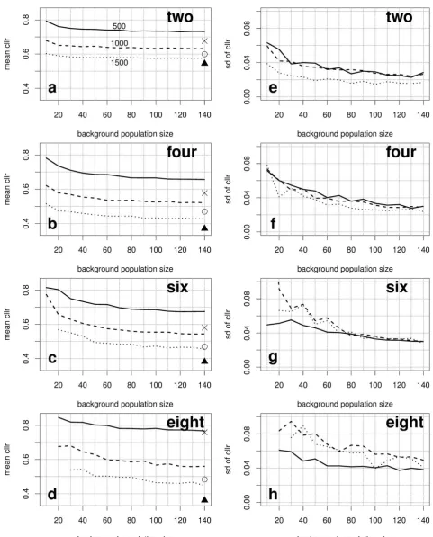
The experimental results of the Monte Carlo simu-lations are given in Figure 2. In the left column of Figure 2 (Panels a, b, c and d), the mean Cllr values
(of the 200 repeated experiments) are plotted as a function of the author count in the background da-tabase (10, 20, 30, 40, 50, 60, 70, 80, 90, 100, 110, 120, 130 and 140 authors), but separately for the sample size (word lengths) of either 500, 1000 or 1500 words. Panels a, b, c and d of Figure 2 are for the two, four, six and eight features, respectively. The panels on the left-hand side of Figure 2 show how the performance of the system changes as a function of the author count in the background da-tabase.
In the right column of Figure 2 (Panels e, f, g and h), the standard deviation (sd) values of the pooled Cllr values are plotted against the number of
authors in the background database, but separately for the different word counts. Panels e, f, g and h of Figure 2 are again for two, four, six and eight features, respectively. Panels e, f, g and h show how the stability of the system performance fluctu-ates as the author count increases in the back-ground database.
First of all, conforming to the results of the pre-analysis given in §3, as can be seen from the left panels of Figure 2, the results of the simulated ex-periments also show that the performance of the system improves as the word count increases. The
two four six eight
500 0.6765 0.5774 0.5812 0.7590
1000 0.5992 0.4690 0.4694 0.4835
1500 0.5448 0.3697 0.3817 0.3619
above observation is not surprising, but it is novel to see that the three curves included in each of Panels a, b, c and d are more or less parallel to each other within the same feature number. This means that the degree of improvement which re-sulted from the increase in word count is there or thereabouts constant, regardless of the author count in the background database.
Further relating to the left panels of Figure 2, although there are some minor ups and downs, the system performance improves, regardless of the number of words and features, as the author count increases in the background database. More pre-cisely speaking, the improvement is in a decelerat-ing manner; there is a large improvement at the beginning, after which the performance starts con-verging or continues to improve to a (far) less de-gree. In the case of the feature number of two (Panel b), for example, there is a minor improve-ment from the author count of 10 to that of 20-30, after which the Cllr values almost remain
un-changed. Whereas for the feature number of four (Panel b), there is a large drop in Cllr value
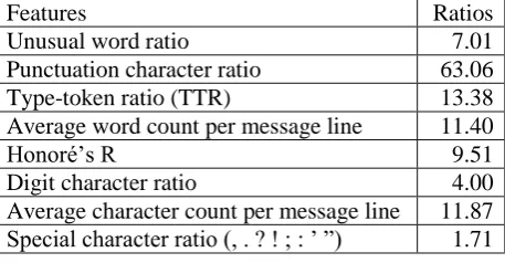
be-tween the author counts of 10 and 50-60, but with 60 authors or more, the degree of improvement is small and linear. That is to say, the more features used for modelling, the more data is required in the background database for the system performance to start converging. However, if the discriminating potential of each feature differs significantly, the above point may not be valid. Thus, the variance ratio (between-speaker sd2/mean within-speaker sd2) (Rose et al., 2006); the greater the ratio is, the higher the discriminating potential of the feature, was calculated for each feature, and given in Table 3.
Features Ratios
Unusual word ratio 7.01
Punctuation character ratio 63.06
Type-token ratio (TTR) 13.38
Average word count per message line 11.40
Honoré’s R 9.51
Digit character ratio 4.00
[image:7.595.67.296.561.680.2]Average character count per message line 11.87 Special character ratio (, . ? ! ; : ’ ”) 1.71
Table 3: Variance ratios.
As can be seen from Table 3, the features of “Digit character ratio” and “Special character ra-tio” are relatively low in variance ratio in
compari-son to the other features. These poor-performing features (variance ratio: 4.00 and 1.71, respective-ly) may have functioned as noise features in the six and eight features, and the inclusion of them may not have contributed to the improvement of the system performance; thus consequently the system may have required more samples to continue to improve in the six and eight features. This entails further study.
Some values are missing in Panels c (six fea-tures) and d (eight feafea-tures) – and consequently in Panels g and h – with the author counts of 10 and 20. This is because all of the relevant 200 repeated experiments returned one or more log10LR = inf or
–inf, which is an ill-condition for the calculation of
Cllr. It is well known that for the higher the
dimen-sion of the feature vector, the more data is required to appropriately model the multi-dimensional den-sity (Silverman, 1986, pp. 93-94). The occurrence of log10LR = inf or –inf indicates that having only
10-20 authors in the background database is not large enough to accurately model the multi-dimensional density of the background population with the feature numbers of six and eight.
As for the stability of the system, an unexpected observation can be made from the right-hand side panels of Figure 2 in that the system does not nec-essarily become more stable in performance (= smaller sd values) with more words in each mes-sage group. This somehow disagrees with the ear-lier observation regarding the system performance and the word count in each message group. For example, the three curves included in Panel f over-lap with each other to a reasonable extent, which means that the system shares a similar degree of stability in performance across the three different word counts, whereas in Panel h, the system with 500 words exhibits smaller sd values (better stabil-ity) on the whole than the systems with 1000 and 1500 words.
These results are counter-intuitive as one would ideally expect that the performance will be more stable with more samples. However, Morrison (2011) notes that in practice this is not often the case. There seems to be some degree of trade-off between the performance in accuracy (which can be represented by Cllr) and the stability of the
sys-tem.
the system performance becomes more stable as the sample size in the background database in-creases; a large improvement in stability at the be-ginning, but the degree of improvement in stability becomes less and less with more authors included in the background database. Additionally, similar to the system performance, it appears in many cas-es that for the stability to start converging, the sys-tem needs more authors in the background database with more features. This point can be seen in Panels e, f and g (1000 and 1500 words), in which the degree of falling in sd values becomes sharper as the feature number increases.
Although the usefulness of the GMM-based Monte Carlo simulation was discussed for the pur-pose of the current study, there is always the possi-bility that the GMM model did not accurately approximate the true nature of the original raw da-ta. In particular, it needs to be pointed out that the system with the synthesised data, on average, un-derperformed the system with the original raw data (refer to Figure 2). However, it is not clear at this stage to what extent and how this possible inaccu-racy of the GMM model influenced the results.
5 Conclusion
By generating synthetic data for the background database by means of the Monte Carlo technique, this study looked into how the performance of the system and its stability are subject to the sample size (= the number of authors) in the background database. The effect of the background sample size on the system performance and stability may differ with the dimensions of the feature vector and the number of words used for modelling. Thus, four different vectors consisting of two, four, six and eight features were tested in this study. Further-more, the number of words used for modelling each message group was also altered as 500, 1000 and 1500 words.
Regardless of the number of features (two, four, six and eight) and words (500, 1000 and 1500), the performance of the system improved in a deceler-ating manner as the sample size (the number of authors) increases in the background database. This result conforms to previous studies on other types of evidence (Hughes et al., 2013; Ishihara & Kinoshita, 2008). Moreover, in general terms, it was found that the more features included in the vector, the more authors the system needs in the
background database for the performance to start converging. However, other potential factors which may have contributed to the outcomes of the current study have also been discussed.
Although there are a large number of potential features that can be used in casework – according to Abbasi and Chen (2008), the total number of features tested in previous studies exceeds 1000, the results of the current study indicate that more features may only deteriorate the performance of the system unless an appropriate amount of back-ground data is available for the dimension of the feature vector, and that the number of features should be determined according to the size of the available background data. These two points are important, in particular, as data scarcity is a com-mon issue in FTC casework. Some drawbacks aris-ing from the use of the GMM-based approximation were also discussed.
It was also pointed out that the model is likely to be inaccurately built only with 10 or 20 authors when the feature number is six or more, resulting in the system returning erroneous LR values. To-gether with other observations, it can be judged that a system with 20 or less authors in the back-ground database is not admissible in court in terms of performance.
In terms of the stability of the system perfor-mance, it is interesting to know that having more words in each message group does not necessarily lead to an improvement in stability. This point was in fact reported in previous studies (Frost, 2013; Ishihara, 2014a; Morrison, 2011). On the other hand, like the case of system performance, regard-less of the number of features and words, it was shown that the system becomes more stable along with the number of authors in the background da-tabase.
The MVKD formula was used in this study. However, there are other methods for estimating LRs (e.g. word or character N-grams) (cf. Ishihara, 2014a; Ishihara, 2014c). This warrants further studies on the same topic as the current study with other methods for LR estimations.
Acknowledgments
The author thanks the three anonymous reviewers for their valuable comments.
References
Abbasi, A., & Chen, H. (2008). Writeprints: A stylometric approach to identity-level identification and similarity detection in cyberspace. ACM Transactions on Information Systems, 26(2), 1-29. Aitken, C. G. G., & Lucy, D. (2004). Evaluation of trace
evidence in the form of multivariate data. Journal of the Royal Statistical Society Series C-Applied Statistics, 53, 109-122.
Balding, D. J. (2005). Weight-of-evidence for Forensic DNA Profiles. Hoboken, N.J.: John Wiley & Sons. Brümmer, N., & du Preez, J. (2006).
Application-independent evaluation of speaker detection.
Computer Speech and Language, 20(2-3), 230-275. De Vel, O., Anderson, A., Corney, M., & Mohay, G.
(2001). Mining e-mail content for author identification forensics. ACM Sigmod Record, 30(4), 55-64.
Evett, I., Lambert, J., & Buckleton, J. (1998). A Bayesian approach to interpreting footwear marks in forensic casework. Science & Justice, 38(4), 241-247.
Fishman, G. S. (1995). Monte Carlo: Concepts, Algorithms, and Applications. New York: Springer. Frost, D. (2013). Likelihood Ratio-based Forensic Voice
Comparison on L2 Speakers. (Unpublised Honours thesis), The Australian National University, Canberra.
Hughes, V., Brereton, A., & Gold, E. (2013). Reference sample size and the computation of numerical likelihood ratios using articulation rate. York Papers in Linguistics, 13, 22-46.
Iqbal, F., Binsalleeh, H., Fung, B., & Debbabi, M. (2010). Mining writeprints from anonymous e-mails for forensic investigation. Digital Investigation, 7(1), 56-64.
Ishihara, S. (2012). Probabilistic evaluation of SMS messages as forensic evidence: Likelihood ration based approach with lexical features. International Journal of Digital Crime and Forensics, 4(3), 47-57. Ishihara, S. (2014a). A comparative study of likelihood ratio based forensic text comparison procedures: Multivariate kernel density with lexical features vs. word N-grams vs. character N-grams.Proceedings of the 5th Cybercrime and Trustworthy Computing Conference, 1-11.
Ishihara, S. (2014b). A likelihood ratio-based evaluation of strength of authorship attribution evidence in SMS messages using N-grams. International Journal of Speech Language and the Law, 21(1), 23-50.
Ishihara, S. (2014c). A likelihood ratio based forensic text comparison in SMS messages: A fused system with lexical features and N-grams. In H. R. Nemati (Ed.), Analyzing Security, Trust, and Crime in the Digital World (pp. 208-224): IGI Global.
Ishihara, S. (2014d). Predatory Chatlog messages as forensic evidence in court: A comparison of two different procedures for estimating the weight of evidence. Proceedings of the 45th Australian Linguistic Society Conference, 131-152.
Ishihara, S., & Kinoshita, Y. (2008). How many do we need? Exploration of the population size effect on the performance of forensic speaker classification. Proceedings of Interspeech 2008, 1941-1944. Marquis, R., Bozza, S., Schmittbuhl, M., & Taroni, F.
(2011). Handwriting evidence evaluation based on the shape of characters: Application of multivariate likelihood ratios. Journal of Forensic Sciences, 56(Supplement 1), S238-242.
Morrison, G. S. (2009). Forensic voice comparison and the paradigm shift. Science & Justice, 49(4), 298-308.
Morrison, G. S. (2011). Measuring the validity and reliability of forensic likelihood-ratio systems.
Science & Justice, 51(3), 91-98.
Morrison, G. S. (2013). Tutorial on logistic-regression calibration and fusion: Converting a score to a likelihood ratio. Australian Journal of Forensic Sciences, 45(2), 173-197.
Neumann, C., Champod, C., Puch-Solis, R., Egli, N., Anthonioz, A., & Bromage-Griffiths, A. (2007). Computation of likelihood ratios in fingerprint identification for configurations of any number of minutiae. Journal of Forensic Sciences, 52(1), 54-64. Robertson, B., & Vignaux, G. A. (1995). Interpreting Evidence: Evaluating Forensic Science in the Courtroom. Chichester: Wiley.
Rose, P. (2013). More is better: Likelihood ratio-based forensic voice comparison with vocalic segmental cepstra frontends. International Journal of Speech Language and the Law, 20(1), 77-116.
Rose, P., Kinoshita, Y., & Alderman, T. (2006). Realistic extrinsic forensic speaker discrimination with the diphthong /ai/. Proceedings of the 11th Australian International Conference on Speech Science and Technology, 329-334.
Silverman, B. W. (1986). Density Estimation for Statistics and Data Analysis. London; New York: Chapman and Hall.