Published online September 20, 2014 (http://www.sciencepublishinggroup.com/j/sr) doi: 10.11648/j.sr.20140204.12
ISSN: 2329-0935 (Print); ISSN: 2329-0927 (Online)
MHD channel flow with skewed applied magnetic
induction field
Frederick J. Young
Department of Communications and Arts, University of Pittsburgh at Bradford, PA
Email address:
[email protected]To cite this article:
Frederick J. Young. MHD Channel Flow with Skewed Applied Magnetic Induction Field. Science Research.
Vol. 2, No. 4, 2014, pp. 62-77. doi: 10.11648/j.sr.20140204.12
Abstract:
The effects of the constant applied magnetic field as a function of its angle with the channel walls is studied using finite elements. This is done for insulating channel walls and for two insulating and two conducting walls forming a short-circuited magnetohydrodynamic generator. The volumetric flow rate is kept constant by regulating the pressure gradient as a function of the applied magnetic induction angle. The necessary pressure gradient diminishes as the angle increases from 0 to 45 degrees because the electrical current flow diminishes. This paper affords a simple and quick method for solving MHD generator problems that defied solution for many years.Keywords:
Magnetohydrodynamic, Generator, Channel, Insulating and Conducting Walls, Skewed Induction1. Introduction
Much has been written about channels carrying conducting fluids[l-22]. Bozkay and Tezer-Sezgin[22] are among the first to investigate the MHD channel with a skewed magnetic field. Their solution is done for only one angle of tilt and they do not consider the MHD generator configuration. When a magnetic field is applied to the channel, usually from an external source such as a magnet, the generated currents alter the velocity profile. To find the altered velocity profile, the usual fluid flow equations must be coupled with the Maxwell equations describing the generated electrical currents that alter the velocity profile. The applied magnetic fields used in most of the papers in the literature are directed along two of the parallel walls of the channel and are perpendicular to the other walls. In this paper the magnetic field is applied at an angle to the walls. A channel with ideally insulating walls and a short-circuited magnetohydrodynamic generator configuration comprising two insulating walls and two ideally conducting is considered. In the MHD generator half of the current returns above and below the generator. Where the current returns affects the induced magnetic induction field which in turn influences the velocity profile. A multitude of other cases could be considered, but are not presented here for brevity.
2. Magnetohydrodynamic Equations
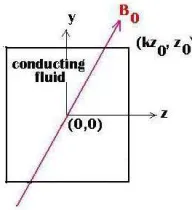
The geometry is shown in Fig. 1. The conducting fluid flows in the x direction under the action of a constant pressure gradient. The applied steady magnetic induction, BO is depicted at an angle to the z axis. Due to symmetry it is sufficient to solve the problem for /4 ≤ ≤ /2
where is the angle between the y axis and the magnetic induction, BO. As in the case where BO is parallel to one of the channel walls, conducting fluid flowing in the x direction and passing through a magnetic field in the yz plane induces electric fields in the yz plane given by Maxwell's curl(H) equation combined with the special theory of relativity as shown below. Here we choose an observer travelling in the fluid. There results
∇x H = -z Hx/ y + y Hx/ z (1)
where Hx is the induced magnetic intensity. Then the
current densities in the y and z direction are given by Jy = Hx/ z (2)
and
Jz = - Hx/ y (3)
The above quantities are seen by an observer riding on the channel walls and those seen by an observer riding in the conducting fluid are denoted with an asterisk. The Maxwell-Lorentz transformation based upon special relativity yields
J* = J = σ(E* + V x B) (4) where J is the same to both observers. Because Ohm's law is good only in the rest frame of the moving conductor, it must be used as given in Eq.4. From the V x E = 0 it follows that
Ez / y = Ey / z (5) Because the velocity,U is in the x direction and the applied magnetic field in the yz plane
V x B = U(-yBOz + zBOy ) (6)
Let H = h + BO/µO where H is the total magnetic intensity vector, h is the induced magnetic intensity and BO is the applied magnetic induction. Also we assume B = h+BO where B is the total magnetic induction and h is the induced magnetic induction that is very small compared to B. Eq.3 becomes
hx/ y = -<(Ez + U BOy ) (7) Substituting Jy as given in Eq.4 into Eq.2 yields
hx/ z = <(Ey - U BOz ) (8)
Eq.7 is differentiated with respect y to yield
2
hx/ 2y = -σ Ez / y - σ (BOy U/ y + U BOy / y) (9)
and Eq.8 is differentiated with respect z to yield
2
hx/ 2z = σ Ey / z - σ (BOz U/ z + U BOz / z) (10)
The addition of Eq.9 and Eq.10 when the V x E = 0 from Eq.5 and V · B = 0 are also substituted gives
∇ hx + σ (BOy U/ y + BOz U/ z) = 0 (11)
which is the magnetohydrodynamic magnetic diffusion equation that must be solved simultaneously with the appropriate Navier-Stokes equation. The induced currents in the fluid cause a retarding force on the fluid given by
J x B = -Jz BOy + Jy BOz = BOy ( hx/ y) + BOz ( hx/ z) (12)
Using this as the electromagnetic body force in the Navier-Stokes equation for the U, the x component of fluid velocity yields
µf ∇ U + BOy ( hx/ y) + BOz ( hx/ z) = P/ x (13)
where P/ x is the pressure gradient that propels the fluid. When the magnetic induction is parallel to one of the walls of Fig.1, Eq.11 and Eq.12 reduce to the standard channel flow equations given by Hughes and Young [l9] at page 199.
3. Boundary Conditions
Considering ideal insulating and conducting walls there are many configurations for a rectangular channel. The boundary condition on velocity at a fixed channel wall is U = 0. If the walls are electrical insulators the induced current circulates inside the channel, never exiting and produces no magnetic field at the walls. Then hx = 0 at all of the boundaries. For conducting boundaries the normal derivative of induced magnetic intensity is zero or hx/ n = 0.
4. Insulating Walls Solution
This is the simplest case when the applied magnetic induction is in either the y or z direction. Then the solution is found by standard methods for solving simple coupled partial differential equations[l9] executed at page 204. The resulting solutions involve infinite series of cisoidal and hyperbolic functions that shed little light on the physical results without rather tedious calculations. The equations presented here for solution do not have constant coefficients and it is not clear that analytical solutions are possible. If they were they might be very hard to evaluate numerically. For example By = BO cos = yBO (y2 + z2)-l/2 and Bz = zBO (y2 + z2)-l/2 would make the solutions to the partial differential equations given above rather difficult. The easy method of solution is to use a finite element numerical solution which is very useful in a closed boundary problem. Here FLEXpde software published by www.PDEsolutions.com is used.
4.1. Finite Element Program
occurring after! Lines 25 through 28 describe the geometry and set the boundary conditions. Line 27 starts at the lower left side of the geometry and value(U)=0 value(h)=0 sets the fluid velocity and the induced magnetic intensity to zero on the complete channel boundary. When starting a new problem it is best to omit lines 3 and 4 to get a quick and rough solution. Line 3 sets the error limit and line 4 requests cubic rather than quadratic elements. Lines 30 and 31 allow the operator to see the solutions as they are done. Lines 32 to 37 produce plots of the contours of U and h and a vector plot of the current density, J. Line 37 a plot of Pg vs .
{1} TITLE 'Magnetohydrodynamic Insulating Channel Flow (MHDIC1.pde)'
{2} SELECT {3} errlim = 1e-04 {4} cubic = on {5} COORDINATES {6} CARTESIAN( 'z' , 'y' ) {7} VARIABLES
{8} U {9} h
{10} GLOBAL VARIABLES {11} Pg ! pressure gradient {12} DEFINITIONS
{13} k = 1 sigma = 1.016E6 ! mercury @ 20 C {14} muf = 1.55E-03 ! mercury
{15} theta = staged(0,5,10,15,20,25,30,35,40,45) {16} sang = Pi*theta/180
{17} B0y = 0.002*cos(sang) B0z = 0.002*sin(sang) ! in tesla
{18} Bm = (B0y^2+B0z^2)^0.5 {19} J = curl(h)
{20} Qcontrol=integral(U) { the control function for
total flow volume } {21} EQUATIONS
{22} U: muf*div(grad(U)) + B0y*Dy(h)+B0z*Dz(h) = Pg ! Eq.13
{23} H: div(grad(H)) + sigma*(B0y*Dy(U)+B0z*Dz(U)) = 0 !Eq.11
{24} Pg: Qcontrol = -50 {determines the negative pressure gradient}
{25} BOUNDARIES {26} region 1
{27} start(0,0) value(U)=0 value(h)=0 line {28} to (1,0) to (1,1) to (0,1) to finish {29} MONITORS
{30} contour(U) report(Bm) report(theta) report(Pg) {31} vector(J) norm report(Bm) report(theta) report(Pg) {32} PLOTS
{33} contour(U) as 'Velocity Profile' report(Bm) report(theta) report(Pg)
{34} contour(h) as 'Induced Magnetic Intensity' report(Bm) report(theta) report(Pg) report(integral(-Dy(h))) {35} vector(J) norm as 'Current Density Vectors' report(Bm) report(theta) report(Pg)
{36} HISTORIES
{37} history(Pg) vs theta as 'Pressure Gradient' {38} END
4.2. Velocity Profiles
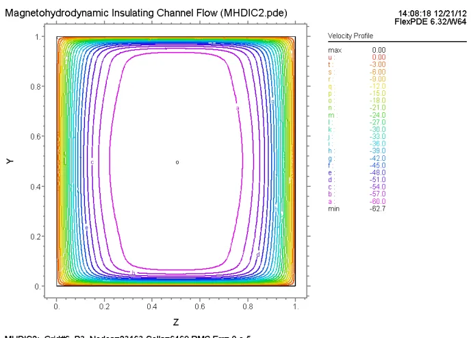
The velocity profiles for = 0, 15, 30 and 45 degrees are presented here. When the reader makes his own calculations using this software smaller increments of angle can be used to produce movies of the velocity profile as e varies.
Figure 3. Velocity profile for = 15 degrees.
Figure 5. Velocity profile for = 45 degrees.
Figure 6. Magnetic intensity for = 0°.
4.3. Induced Magnetic Intensity
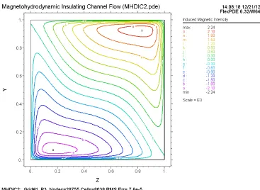
The induced magnetic intensity, hx is also plotted for the same values of e. The lines of constant magnetic intensity are the lines of current flow and like the velocity profile the
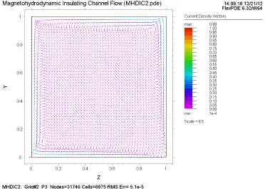
45o. This is illustrated in Fig.10 showing the current density vectors. In line 35 of the script the word 'norm' makes all the vectors the same length. If that word were not there, the vector lengths would be proportional to the true length of the vectors that might be too small to see. However, when all the vectors are the same length their colors indicated their true magnitude. Most of the current
flows in a boundary layer near the insulating walls and returns in the core of the flow to generate a negative magnetic intensity near (0.1,0.1) and a positive magnetic intensity near (0.9,0.9). The total flow has been kept constant by adjusting the pressure gradient as the angle of the applied magnetic induction is varied. The adjusted pressure gradient is shown in Fig.11. The adjustment is.
Figure 7. Magnetic intensity for = 15°.
Figure 9. Magnetic intensity for = 45°.
Figure 10. The current density vectors for = 45° not large.
5. Verification of Eq.11 and Eq.13
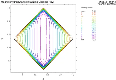
Both of these equations have an extra term compared to the conventional MHD channel equations. A method to check them is to rotate the channel so that the extra terms are not needed. Here the channel is rotated by 45 degrees
the same extremum values of magnetic intensity. Fig. 14 Show the current density vectors that are the same as those of Fig.10. Most of the current flows in a layer near the insulating boundaries and returns at low density through
the fluid core forming two oppositely directed eddies. These results show that the extra terms here in the MHD equations are correct.
Figure 11. Adjusted pressure gradient vs e.
6. Conducting and Insulating Walls
6.1. A Magnetohydrodynamic Generator Configuration
For all walls U = 0. If the top and bottom walls are insulators the magnetic intensity at the top wall should be equal to the negative of the magnetic intensity at the bottom wall when one-half of the current returns above and one-half returns below the channel. This is an antiperiodic condition easily done with finite elements. At the electrodes walls located on the xy plane at z = 0 and z = 1, the boundary conditions are 8hx/8z = 0. In this case lines 27 and 28 of the script should be:
{27} start(0,0) value(U)=0 nobc(h) line to (1,0) natural(h)=0 line to (1,1)
{28} value(h)=0 antiperiodic(z,y-1) line to (0,1) value(U)=0 nobc(h) line to finish
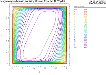
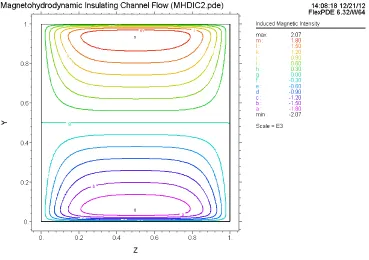
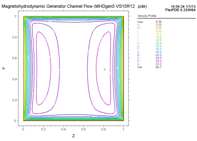
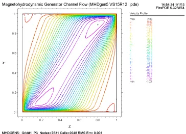
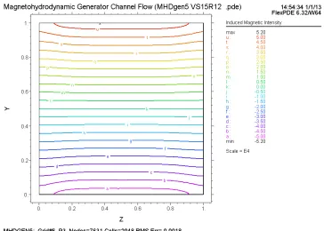
This change invokes antiperiodicity and the nobc(h) allows the values of h to be calculated so that they are of the same magnitude but of differing sign at the top and bottom boundaries. The comparison of Figures 15 through 18 shows a skewing of the core of the velocity that increases with the angle of the applied magnetic induction. Figures 19 through 22 show the magnetic intensity or
current lines as the angle increases. As expected the current flows across the channel in the z direction in all cases. However, as the angle, e increases the current lines become distorted and tend to flow perpendicular to the channel diagonal, only resuming flow directed more in the z direction near the electrodes at z=0 and z=1. In Fig. 23 the current density vectors are displayed for e = 45o. Note the skewing along the diagonal and the development of eddies at the lower left and upper right corners of the channel.
In these calculations 181 stages (one for each 1/4 degrees of angle) were made so that movies of the above curves could be produced with appropriated frame rates. Those who have downloaded Flexpde demo version are encouraged to run this problem and view the movies. Having kept the volumetric flow rate constant by regulating the pressure gradient, it is of interest to have a curve of pressure gradient versus angle. This was done in the HISTORY section of the script. Fig.24 shows the pressure gradient diminishing as e increases from 0 to 45 degrees whereas Fig.25 exhibits the magnitude of the current decreasing. As the current decreases the J x B decreases making it require less pressure gradient to push the fluid through the channel. Thus the aforementioned curves Behave in accordance with physical principles.
Figure 14. Current density vectors.
Figure 16. Velocity profile for e = 15°.
Figure 18. Velocity profile for e = 45°.
Figure 20. Magnetic intensity for = 15.
Figure 22. Magnetic intensity for = 45°.
Figure 24. Pressure gradient versus .
Figure 25. Total current versus .
7. Conclusions
The finite element solution to the channels considered here, is easily applied and the results can be presented graphically in as much detail as desired. This is in contrast to finding closed form solutions to the
Research in magnetohydrodynamic generators has diminished because of material problems. They can be activated at full power for only a few minutes before they burn away. However, if power is needed in a very remote location where no electric power lines exist and power is needed for only one or two minutes for a rocket launch such a disposable magnetohydrodynamic generator would be very useful. The solution presented here can also be used to account for the fringing of the applied magnetic field encountered in all practical magnets.
From the curves presented here it is clear that skewing the magnetic induction field does not help but rather hinders the magnetohydrodynamic flow by effectively lowering the Hartmann number.
In contrast to most papers in this field the reader can do a very large number of very different cases by using the included computer program that can be easily modified. Many published papers seem to be of interest and useful but the reader of most of them finds it very difficult to repeat their work and almost impossible to easily do new cases. It is easy to get a student version of FlexPDE at no cost from www.pdesolutions.com. The program is easily modified to include loads on the MHD generator and can account for fringing of the magnetic induction. The program given here runs on said student version. However, the curves it produces are not a smooth as those produced by the professional version that can be obtained on a trial basis.
References
[1] B.Singh, J. Lal, MHD axial flow in a triangular pipe under transverse magnetic field, Ind. J. Pure Appl. Math. 9 (1978) 101-115.
[2] B.Singh, J. Lal, MHD axial flow in a triangular pipe under transverse magnetic field parallel to a side of the triangle, Ind. J. Technol. 17 (1979) 184-189.
[3] B.Singh, J. Lal, Finite element method for MHD channel flow with arbitrary wall conductivity, J Math. Phys.Sci. 18 Applied Mathematics 2012, 2(3): 58-65 65 (1984) 501- 516.
[4] L.R.T. Gardner, G.A. Gardner, A two-dimensional bi-cubic B-spline finite element used in a study of MHD duct flow, Comput Methods Appl. Mech. Eng. 124(1995) 365- 375.
[5] M. Tezer-Sezgin, S. Koksal, FEM for solving MHD flow in a rectangular duct, Int. J. Numer. Meth. Fluids 28 (1989) 445-459.
[6] Z. Demendy, T. Nagy, A new algorithm for solution of equations of MHD channel flows at moderate Hartmann numbers, Acta Mechanica 123 (1997) 135- 149.
[7] K.E. Barrett, Duct flow with a transverse magnetic field at
high Hart- mann numbers. Int. J. Numer. Meth. Fluids 50 (2001) 1893-1906.
[8] M. Tezer-Sezgin, BEM solution of MHD flow in a rectangular duct, Internat. J. Numer. Methods Fluids 18 (1994) 937-952.
[9] H.W. Liu, S.P. Zhu, The dual reciprocity boundary element method for magnetohydrodynamic channel flows, ANZIAM J. 44 (2) (2002) 305-322.
[10] A. Carabineanu, A. Dinu, I. Oprea, The application of the boundary element method to magnetohydrodynamic duct flow, ZAMP 46 (1995) 971-981.
[11] C. Bozkaya, M. Tezer-Sezgin, Boundary element solution of unsteady magnetohydrodynamic duct flow with differential quadrature time integration scheme, Int. J. Numer. Meth. Fluids 51 (2006) 567-584.
[12] M. Tezer-Sezgin, Solution of magnetohydrodynamic flow in a rectangular duct by differential quadrature method, Computers 8 Fluids 33 (2004) 533-547.
[13] H. Korogulu, Chebyshev series solution of linear Fredholm integrodifferential equations, Int. J. Math.Educ.Sci.Techno. 29(4) (1998) 489-500.
[14] M. Dehghan, D. Mirzaei, Meshless local boundary integral equation (LBIE) method for the unsteady magnetohydrodynamic (MHD) flow in rectangular and circular pipes, Comput. Phys. Commun. 180/9 (2009) 1458-1466.
[15] I. QELIK, Solution of magnetohydrodynamic flow in a rectangular duct by Chebyshev collocation method, International Journal for Numerical Methods in Fluids, 66 (2011) 1325-1340.
[16] C. C. Chang and T. S. Lundgren, Duct flow in magnetohydrodynamics, Z. angew. Math. Phys. 12 p. 100 (1961)
[17] R. R. Gold, Magnetohydrodynamic pipe flow, Part 1, J. Fluid Mech., 13 p. 505 (1962). This paper has a rather complete list of references.
[18] F. J. Young and J. F. Osterle, on the load capacity of hydromagnetically lubricated slider bearing, Wear, 5, p. 227 (1962).
[19] W. F. Hughes and F. J. Young, The electromagnetodynamics of Fluids, John Wiley 8 Sons, Inc. New York (1966) Library of Congress Catalog Number 66-17621.
[20] F. J. Young, The calculation of magnetically induced electromotive force, Xlibris, ISBN 1-4797-3789-5 (2012).
[21] J. A. Shercliff, Steady motion conducting fluids in pipes under transverse magnetic fields, Proc. Cambridge Philos. Soc. 49 (1953) 136-144.