http://www.sciencepublishinggroup.com/j/ijass doi: 10.11648/j.ijass.20190701.11
ISSN: 2376-7014 (Print); ISSN: 2376-7022 (Online)
Study of Response of Extreme Meso-Scale Field-Aligned
Current to Interplanetary Magnetic Field Components B
X
,
B
Y
and B
Z
During Geomagnetic Storm
Adero Ochieng Awuor
1, *, Paul Baki
1, Olwendo Joseph
2, Pierre Cilliers
3, Pieter Kotze
31Department of Physics and Space Science, Technical University of Kenya, Nairobi, Kenya 2
Department of Mathematics and Physical Sciences, Pwani University, Mombasa, Kenya 3
South Africa National Space Agency, SANSA Space Center, Hermanus, South Africa
Email address:
*Corresponding author
To cite this article:
Adero Ochieng Awuor, Paul Baki, Joseph Olwendo, Pierre Cilliers, Pieter Kotze. Study of Response of Extreme Meso-Scale Field-Aligned Current to Interplanetary Magnetic Field Components BX, BY and BZ During Geomagnetic Storm. International Journal of Astrophysics and
Space Science. Vol. 7, No. 1, 2019, pp. 1-11. doi: 10.11648/j.ijass.20190701.11
Received: October 6, 2018; Accepted: November 26, 2018; Published: August 6, 2019
Abstract:
The influence of IMF components on meso-scale field-aligned currents (FACs) is investigated with an aim to establish how different IMF components influence the occurrence and distribution of FACs. The field-aligned currents (FACs) are calculated from the curl of the Ampere’s law to the magnetic field recorded by CHAMP satellite during 24 major geomagnetic storms. To determine the field-aligned currents at extreme mesoscale range ∼150 - 250 km, a low-pass filter to FACs with a cutoff period of 20s is applied. The peak-to-peak amplitude of FAC density, with the maximum difference ≤ 30 MLAT, is determined and used to define the FAC range. The results indicate high occurrence of FACs centered about IMF ≈ 0, for large values of Dst. The magnitude of FACs is in general affected by all the three IMF components, alongside other ionospheric factors such as solar wind speed and density. Magnetic reconnection, under -BZ is a major FACs drivers and issignificant in the dayside northern hemisphere. The reconnection is not symmetric in both hemispheres. We find a possible electrodynamic similarity between the dayside northern hemisphere and nightside southern hemisphere, prominent along BX
when BZ is negative. This interesting observation can further be investigated.
Keywords:
Auroral Ionosphere, High-latitude Current Systems, Magnetosphere-ionosphere Coupling1. Introduction
A number of systems of global-scale electrical currents are generated in the near-Earth environments due to the interaction between the solar wind and interplanetary magnetic field. One of such currents is the field-aligned currents (FACs), commonly referred to as Birkeland currents after he first suggested their existence in the upper atmosphere in 1908. This current system plays a role in coupling the energy from the magnetosphere to the high latitude conducting ionospheres. This coupling can lead to magnetospheric perturbations and currents which have been shown to be the cause of various devastating effects on Earth’s atmosphere, such as, geomagnetically induced
currents (GICs) on power grids, railways, and other long-distance conducting structures [12]. The dynamics of the high-latitude thermosphere is greatly affected by the energy input from the solar wind via Joule heating and particle precipitation [21, 30]. Further, Joule heating of the thermosphere can have undesired effects on satellites in low Earth orbits [7]. These effects result from large currents, totaling approximately 4 MA for typical solar wind and IMF conditions and increasing as more extreme driving occurs [34]. Thus, a better understanding of the FAC distribution under various geomagnetic conditions and IMF orientations is important for understanding energy transfer in the magnetosphere-ionosphere system. The IMF BY component
has been hypothesized to be due to field-aligned currents (FACs) [28]. The effect of polarity of IMF BY on the FACs
topology is reversed in the southern hemisphere due to the antisymmetry of the reconnection site with respect to the noon-midnight meridian [10].
Four types of FACs are known to exist, e.g., Region 1 (R1), Region 2 (R2), northward IMF Bz (NBZ), and IMF BY
modulated (DPY) FACs [16, 17]. R1 FACs flow into the ionosphere in the morning sector and out of the ionosphere in the evening sector, and R2 FACs are located equatorward of the R1 FACs with opposite polarities. For northward IMF Bz, NBZ FACs dominate in the polar cap poleward of R1 FACs [17]. This current system, NBZ FACs, have been interpreted in terms of the antiparallel reconnection on field lines tailward of the dayside cusp [17, 31, 32]. When IMF BY
becomes dominant DPY FACs form around the noon sector while positive BY, in the northern hemisphere results in
upward field-aligned current located poleward of the downward current, and vice versa in the southern hemisphere [16, 2]. The poleward part of DPY currents could be associated with the plasma mantle/cusp precipitation, while the equatorward part is an intrusion of dawnside (BY > 0) or
duskside (BY < 0) R1 currents [e.g., 8, 35]. The high-latitude
ionospheric convection pattern strongly depends on the orientation of IMF [13]. Normally, for southward IMF two-cell convection flow pattern exists, while for northward IMF four-cell flow pattern emerges due to high-latitude reconnection. IMF BY will distort the convection map and
cause dawn-dusk and interhemispheric asymmetries. The locations of the auroral oval and its activity have been found to strongly depend on the IMF configuration [14]. High auroral power is observed for all negative IMF components [29]. A brighter dayside aurora has also been observed for BX< 0 than for BX > 0 during southward IMF, while the
nightside aurora brightness is less dependent on IMF BX, and
the duskside auroral brightness for northward IMF is not so much brighter for BX < 0 than for Bx > 0 [36].
The overall response of both the ionospheric convection and field-aligned current distribution to IMF BZ, BX and BY
has been established. However, the mutual relationship of these components has not been comprehensively examined. The relationship would, for instance, help us understand the mapping of the field-aligned currents from the ionosphere to the magnetosphere. In this study, we will examine the effect of IMF BX, BY, and BZ on the ionospheric distribution of
FACs by defining a new parameter called FAC range. We define FAC range as peak-to-peak amplitude of FAC density, filtered by a 20s low-pass filter. The location of maximum and minimum peaks is determined by the magnetic latitude (MLAT), with the maximum difference ≤ 30 MLAT, alongside the corresponding magnetic local time (MLT) and universal time (UT). The satellite passes with the peaks which are far apart (>30 MLAT) are discarded. This was done to avoid using peaks in different MLT sectors. The FAC range comprises R0, R1 and R2 FACs.
The paper is organized as follows; the data set and methodology are described in section 2. The results are
presented in section 3 while section 4 outlines the discussions. Finally, the conclusion is given in section 5.
2. Data Set and Methodology
2.1. CHAMP Satellite Data
The geoscientific satellite CHAMP was launched on 15 July 2000 into a near circular, near-polar orbit (87.30 inclination) [23, 25]. With initial altitude at 456 km the orbit decayed to about 350 km after 5 years. The orbital plane precesses at rate of 1 h in local time (LT) per 11 days, thus covering all local times within 131 days. The data used here are the vector magnetic field measurements of the Fluxgate Magnetometer (FGM). FGM instrument delivers vector field readings at a rate of 50 Hz. The satellite data used in this study are the pre-processed (level 2) fluxgate magnetometer vector data from CHAMP in sensor frame (product identifier CH-ME-2-FGM-FGM), which has been down sampled to 1.0 Hz.
2.2. Geomagnetic and OMNI IMF/Solar Wind Data
The Dst, IMF BZ (in GSM coordinates) and solar wind
dynamic pressure are taken from NASA/Goddard Space Flight Center’s (GSFC’s) OMNI data set through the OMNIWeb interface. The OMNI data set provides time series of solar wind parameters propagated to their impact on the bowshock [24]. The solar wind data has been time shifted for 15 min to take into account the solar wind propagation through the magnetosheath from the bow shock nose to the magnetopause [5].
2.3. Field-Aligned Currents Density Calculation
The FAC density is determined according to Ampere’s law from the vector magnetic field data by solving the curl-B, that is, = − where is the vacuum permeability, Bx and By are the transverse magnetic field deflections caused by the currents. We have assumed that FACs is infinite sheets aligned with the mean location of the auroral oval [33]. Since we do not have multipoint measurements, we convert spatial gradients into temporal variations by considering the velocity under the assumption of the stationary of the current during the time of satellite passage. After discrete sampling is introduced, we obtain
= where vx is the velocity perpendicular to the
current sheet and By is the magnetic deflection component parallel to the sheet [22].
3. Observations
3.1. IMF-FAC Range Variation in Different MLT Sectors
The Figures 1-8 show the variations of FAC range with IMF BX, BY and BZ components. The data are classified
MLT), dawnside (0500-0700 MLT) and duskside (1700-1900 MLT). We however take note of relatively limited number of data points for some MLT sectors, which could lead to uncertainties in the interpretations.
From left to right, the panels in Figures 1-8 correspond to IMF BX, BY and BZ while from top to bottom, we have
dayside, nightside, dawnside and duskside sectors respectively. Indeed, the IMF BX and BY component affect
both dayside and nightside Polar Regions. The increase of FAC range magnitude corresponded fairly well to an increasing |BZ| during southward IMF, while the magnitude
remained fairly constant regardless of |BZ| during northward
IMF, clearly seen on the nightside MLT sector. The other IMF components, on the hand, did not show, in general, the increasing FAC range magnitude with increasing IMF.
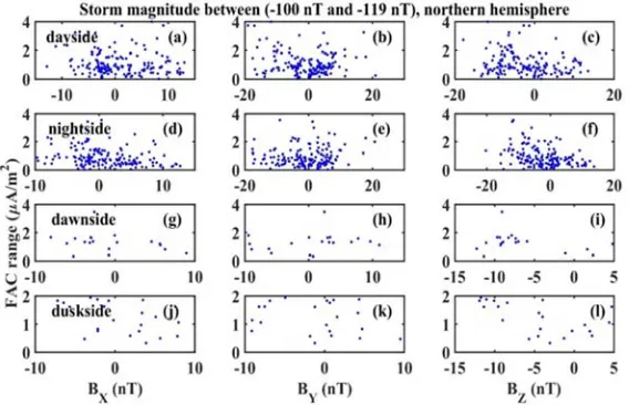
Figure 1. FAC range against various IMF components. Panels a, b and c (dayside), d, e and f (nightside), g, h and i (dawnside) and j, k and l (duskside) in the northern hemisphere. The Dst value between −119 −100.
The distribution of FAC range varied differently in all MLT sectors for different IMF components, depending of the negative and positive deflection of the components. Higher FAC range occurrence is exhibited during positive IMF BX
than during negative IMF BX during the dayside MLT sector
and the reverse is observed in the nightside. For the IMF BY
component, higher occurrence of FAC range is observed when the component is negatively deflecting than during positive deflecting. The reverse is observed during the dawn MLT sector. Figure 1 (c and f panels) show IMF BZ, as
expected, higher occurrence of FAC range with larger densities is observed during the negative deflection than during the positive deflection. The occurrence of FAC range
is also higher during the dayside MLT sector than the rest of other sectors.
The magnitude of FAC range density increased significantly, possibly responding to the increase in storm magnitude. The increase is more pronounced during the dayside (Figure 2, a-c) MLT sectors. High FAC range occurrence is observed during the negative IMF BX in all
MLT sectors while for IMF BY the distribution is almost
symmetrical about IMF BY ≈ 0, but with high magnitudes of
FAC range during the negative IMF BY. The response of FAC
range distribution observed during the negative IMF BZ is
consistent throughout the MLT sectors.
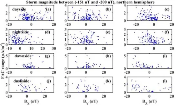
Figure 3. Same as Figure 1 for Dst value between−200 −151.
The magnitude of FAC range did not respond significantly to the decrease in the storm main phase (−151
−200 !. The distribution of FAC range is however showing meaningful differences in different MLT sectors. While during the dayside, the occurrence of FAC range is higher for negative deflection of IMF BX (Figure 3a) and IMF
BZ (Figure 3c) than during the positive deflections in both
cases, the IMF BY (Figure 3b) is centered about IMF BY ≈
±5nT. The nightside MLT sector exhibited the same trend. Both dawnside and duskside MLT sectors showed negative deflections of IMF components to favor the occurrence of the FAC range compared to positive deflection.
Figure 4. Same as Figure 1 for Dst value " −200 .
Figure 4, panels (d-f), show significant increase in the FAC range magnitude. The most remarkable difference is observed during the dayside MLT sector, panels (a-c), where the distribution of FAC range is almost symmetrical
about−10 #$% 10 . The FAC range intensities are stronger for large positive and negative values of the BZ
(Figure 4, c and f).
There is less occurrence of FAC range in the southern hemisphere compared to similar conditions in the northern hemisphere (Figure 1) with the FAC range distribution about the
−10 #$% 10 . This could imply asymmetry in reconnection in southern and northern hemispheres. Higher FAC range occurrence is exhibited during positive IMF BX than
during negative IMF BX during the dayside MLT sector and the
reverse is observed in the nightside. For the IMF BY component,
higher occurrence of FAC range is observed when the component is negatively deflecting than during positive deflecting. The reverse is observed during the dawn MLT sector. Figure 1(c and f panels) show IMF BZ, as expected, higher
occurrence of FAC range with larger densities is observed during the negative deflection than during the positive deflection. The occurrence of FAC range is also higher during the dayside MLT sector than the rest of other sectors.
Figure 6. Same as Figure 2 in the southern hemisphere.
Figure 6 shows less occurrence of FAC range in all MLT sectors, with higher magnitudes and distributions during negative IMF BZ component compare to during positive IMF
BZ. The IMF BY component exhibited a roughly symmetric
distribution about IMF ≈ 0, spreading wider during the
dayside and nightside MLT sectors compared to dawn-dusk sectors. The IMF BX component had dayside FAC range
distribution and magnitude responding to positive IMF BX
compared to negative IMF BX while the reverse is observed
during the nightside MLT sector (Figure 6d).
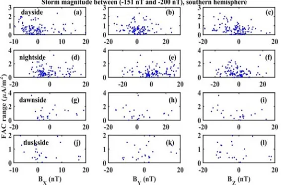
Figure 7. Same as Figure 3 in the southern hemisphere.
The occurrence of FAC range is evidently higher during the
&'" 0, in all MLT sectors. For IMF BY, the dayside MLT
sector (Figure 7b) showed, to some extent, symmetrical distribution of FAC range for both negative and positive deflections. The same is observed during the dusksise MLT sector (Figure 7k). During the nightside MLT sector, the
Figure 8. Same as Figure 4 in the southern hemisphere.
The distribution of FAC range tends to concentrate between
−10 #$% 10 for dayside and nightside MLT sectors. The same trend is exhibited in dawnside and duskside sectors though with less symmetric distribution about the IMF ≈ 0. The dayside MLT sector still exhibited higher occurrence of FAC range compared to nightside sector. The magnitude of FAC range did not vary much correspondingly to the increase in Dst.
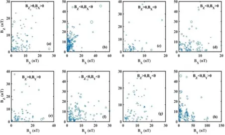
3.2. Day-night FAC Range Dependence on the Orientation of IMF
In this section, we investigate the FAC range cases in IMF
BX-BZ and IMF BY-BZ planes in different orientations
(positive and negative deflections) in northern and southern hemispheres. The position of the circle is determined by the corresponding values of the IMF components while the size of the circle represents the magnitude of the FAC range. The IMF orientations are categorized as +&* ) 0, &') 0! ,
+&*" 0, &' " 0!, +&*) 0, &' " 0! and +&* " 0, &') 0! for IMF BX-BZ plane and the same conditions are considered
for IMF BY-BZ plane.
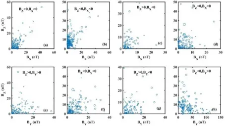
Figure 9. Relationship between the IMF BX, IMF BY and BZ with the FAC range. Area of the circle represents the magnitude of FAC range, dayside northern
hemisphere.
range is prevalent along the IMF BZ compared to IMF BY in
all cases (Figure 9h, 10h, 11h and 12h). This indicates the dominance of negative IMF BZ over positive IMF BY. The
positive IMF BZ component was dominant over negative BX
in the northern hemisphere (Figures 9c and 10c), with more FAC range cases occurring along the IMF BZ > 0. This is not
the case in the corresponding day-night sectors in the southern hemisphere (Figures 11c and 12c). A nearly linear relationship between IMF +BZ and IMF +BX is observed in
both hemispheres, with a clear linear dependence in the northern hemisphere night sector (Figure 10 a, b) and southern day sector (Figure 11a, b), indicating a possible electrodynamic similarities between nightside northern hemisphere and dayside southern hemisphere. The similarity can be further investigated. The FAC range magnitudes are stronger for large -BZ compared to large +BZ. FAC range
occurrence and magnitude seem to favor large values of |IMF BY|, prominent in northern hemisphere than in southern
hemisphere whenever IMF BZ < 0. The north-south
hemispheres asymmetry is observed in the IMF BX
component. The northern hemisphere dayside (Figure 9a) FAC occurrence showed a similar behaviour as the southern nightside FAC cases (Figure 12a). Similar observations are
made between northern hemisphere nightside (Figure 10a) and the dayside FAC range occurrence in the southern hemisphere (Figure 11a).
High occurrence of FAC range is observed for small values of IMF components. For &* ) 0, &') 0, large FAC range density occur when IMF BZ is small and BX ~ 10 nT (Figure
9a). The distribution of FAC range favored the large values of BX, corresponding to large values of BZ. For southward
IMF BZ and negative IMF BX (Figure 9b), the large FAC
range density occurs for large IMF BZ with more cases of
FAC range occurring for small negative IMF BX. Figure 9c
compares FAC range cases for positive IMF BZ and negative
IMF BX. Few cases of FAC range is exhibited under this
condition, with large FAC range density occurring for small BZ and BX. The large FAC range occurred during large
negative IMF BZ (Figure 9d). While comparing the FAC
range occurrence with different orientations of IMF BZ and
IMF BY, the FAC range cases are more prevalent during IMF
BZ < 0, (Figure 9f and 9h). During IMF BZ > 0, larger FAC
range occurred during negative BY (Figure 9g) compared to
positive BY, (Figure 9e). However, the FAC ranges with large
densities tend to occur in the large |IMF BY| and small |IMF
BZ| region in all cases in IMF BZ-BY plane.
Figure 10. Same as Figure 9 for nightside northern hemisphere.
The nightside FAC range seemingly enjoy a linear relationship in the IMF BZ-BX plane, when both components
are positive (Figure 10a). Large FAC range densities are however observed for small IMF BZ and BX. When both
components are negative (Figure 10b), the negative IMF BZ
components dominates in terms of FAC range occurrence and also large values of FAC range are seen during large values of negative IMF BZ. Interchanging the directions of the IMF
components, with positive IMF BZ and negative IMF BX
(Figure 10c) leave no components preferred for the
occurrence of FAC range. The large density FAC range occur for the small values of the IMF components in this condition. For the case of negative IMF BZ and BX > 0 (Figure 10d),
more FAC range occurred along IMF BZ. Large FAC range
density are observed during large values of IMF BZ < 0 and
small IMF BX > 0. In the IMF BZ-BY plane, the occurrence of
FAC range was prevalent in BY component than along BZ
except for IMF BZ < 0 and BY > 0 (Figure 10h). Large FAC
range density occurred during large IMF BZ and small IMF
Figure 11. Same as Figure 9 for dayside southern hemisphere.
The possible linear relationship between the IMF BZ-BX
plane FAC range when both components are possible (Figure 11a) while the larger FAC range are observed for small values of IMF BZ and BX. Similar observations are exhibited when
IMF BZ and BX are negative (Figure 11b). For IMF BZ > 0 and
BX < 0, few cases of FAC range are observed with the large
density FAC range occurring when IMF BZ is very small
(Figure 11c). In Figure 11d, large values of FAC range density are observed during large values of IMF BZ. In the IMF BZ-BY
plane, except for both positive IMF BZ and BY (Figure 11e)
where large values occurred for small values of IMF BZ and
BY, Figure 11f, g and h, shows dominant occurrence of FAC
range along the IMF BZ component. Large values of FAC
range are observed when IMF BY is very small.
Figure 12. Same as Figure 9 for nightside southern hemisphere.
the both large values of IMF BZ and BX positive (Figure 12a)
and IMF BZ and BX negative (Figure 12b). For BZ > 0 and BX
< 0 large FAC range values are observed for large values of IMF BX (Figure 12c). For IMF BZ < 0 and IMF BX > 0, the
large values of FAC range occurred during large values of IMF BZ. The IMF BZ-BY plane had large values of FAC range
when BY was large and small BZ (Figure 12e) while large
values of FAC range are observed for large values of IMF BZ
and small magnitude of IMF BY for IMF BZ < 0, IMF BY > 0
(Figure 12h).
4. Discussions
Interplanetary magnetic field (IMF) influences on the occurrence of large-scale FACs has been long recognized [31, 19, 1]. The IMF influence on the FACs is however not from only a single IMF component but a contribution from all the IMF components. For instance, it has been found that in the polar region the distribution, scale, and magnitude of the Joule heating region, and the corresponding FACs, are controlled mainly by the IMF clock angle, which is determined by the BY and BZ components of the IMF [20].
The occurrences and patterns of the high-latitude field-aligned currents (FACs) observed in Figures 1-12 are an indication of the solar wind-magnetosphere-ionosphere coupling. Using geomagnetic data from CHAMP satellite, during geomagnetic storm, the study has investigated the occurrences and intensifications of FAC range for different interplanetary magnetic field (IMF) orientations and amplitudes for 24 different storms. The intensification of FACs manifested in large magnitudes of FAC range during southward IMF BZ compared to northward IMF BZ (Figures
1-8, IMF BZ column) indicating that the magnetopause is
closer to Earth under southward IMF than under northward IMF BZ. Similar observations are made in IMF planes,
whenever IMF BZ < 0, (Figures 9-12). The dayside sector has
exhibited high occurrences of FAC range indicating significant influence of dayside magnetic reconnection. Magnetic reconnection has also been alluded to as the main driver for strong FACs originating from magnetopause boundary during the southward IMF [15, 4]. This implies that the merging between the IMF and Earth’s magnetic field creates open field lines that are transported tailward by the magnetosheath flow in accordance to [6]. During IMF -BZ,
magnetic flux is removed from the dayside and added into the tail flux tubes. The open flux is then closed by subsequent reconnection in the magnetotail and returned to the dayside by sunward convection. The magnetotail reconnection explains the observed nightside high occurrence of FAC range cases (Figures 1-8, second row).
The influence of the level of geomagnetic activity on FAC range is evident on both hemispheres. With the increase in the activity level (Dst < -200 nT), the FAC range magnitude remains fairly constant for |IMF| (Figures 4 and 8). The observed enhanced fluctuations are consistent with the enhanced FACs reported by [3].
For geomagnetic activity ≥ - 200 nT, Figures 1-3, northern
hemisphere and Figures 5-7, southern hemisphere, the occurrence and magnitude of FAC range fairly depended on the orientation of IMF. This concurs with the observation that high-latitude ionospheric convection pattern strongly depends on the orientation of IMF [13]. The occurrences and intensity of FAC range is higher during the negative deflection of IMF components compared to positive deflection, affirming the observations by [29, 35].
The nightside FAC range showed a clear dependence on IMF BZ (Figures 1f, 2f, 5f, 6f and 7f), with increasing
magnitude of FAC range with increasing IMF -BZ and a
fairly constant FAC range magnitude during IMF +BZ
compared to their dayside counterparts. This apparent dependence on IMF Bz could be due to the relationship between IMF Bz and AL index [9]. A similar observation was also made by [18].
The magnitude of FAC range increased, to some extent, with increasing |IMF BY| while higher occurrence as
observed around −10 ≤ |#$% &(| ≤ 10 during both dayside
and nightside (Figures 1-8). Figures 9-12 also showed increasing occurrence and magnitude of FAC range cases with increasing |IMF BY|, whenever BZ < 0. This affirms that
IMF BY component affects not only the dayside polar region
but also the nightside polar region and consistent with the observations by a number of scholars. The influence of IMF BY on the FACs near the midnight auroral oval, where the
intensity of the currents increases with |BY| was observed by
[27]. Further, the coherent BY-controlled convection exists
near the midnight auroral oval when IMF is stable, and when its magnitude is large, and that the distribution of the FACs is associated with BY-controlled convection [26]. IMF BY
component changes the location of the reconnection site on the magnetopause, leading to a number of asymmetric features. On the dayside, finite IMF BY shifts the dayside
reconnection site from the subsolar point, toward high-latitude flanks, where antiparallel reconnection is dominant.
The north-south asymmetry in the IMF BX component
could be due to the magnetopause reconnection location. For BZ < 0, a positive (negative) BX might be expected to move
the preferred reconnection location northward (southward) along the closed dayside field line. Closed dayside flux may be transferred to open nightside flux and the ionospheric projection would be expected to behave the same way as the southward IMF. For BZ > 0, a positive (negative) BX is
expected to favor open-to-open lobe reconnection in the southern (northern) hemisphere.
5. Conclusion
Although the IMF magnitude affects the magnitude/intensity of FACs, other ionospheric parameters such as solar wind speed and density (not studied here), may also be of great influence. The IMF BX drives the north-south asymmetry, with the north
dayside depicting a similar electrodynamic to the south nightside.
Acknowledgements
The operational support of the CHAMP satellite mission, the World Data Center, Kyoto, the GSFC/SPDF OMNIWeb interface at http://omniweb.gsfc.nasa.gov, from where the data used in this study was obtained, are sincerely acknowledged. This work was also supported by the South Africa National Space Agency (SANSA), Technical University of Kenya (TUK) and the National Commission for Science, Technology and Innovation (NACOSTI).
References
[1] Cheng, Z. W., Shi, J. K., Dunlop, M., & Liu, Z. X. (2013). Influences of the interplanetary magnetic field clock angle and cone angle on the field-aligned currents in the magnetotail.
Geophysical Research Letters, 40(20), 5355–5359. https://doi.org/10.1002/2013GL056737.
[2] Clauer, C. R., and E. Friis-Christensen (1988), High-latitude dayside electric fields and currents during strong northward interplanetary magnetic field-Observations and model simulation, J. Geophys. Res., 93, 2749–2757.
[3] Coxon, J. C., Milan, S. E., Clausen, L. B. N., Anderson, B. J., and Korth, H. (2014). Journal of Geophysical Research : Space Physics A superposed epoch analysis of the regions 1 and 2 Birkeland currents observed by AMPERE during
substorms, 9834–9846.
https://doi.org/10.1002/2014JA020500. Abstract.
[4] Cowley, S. W. H. (2000). Magnetosphere-ionosphere interactions: A tutorial review. Geophysical Monograph Series, 118, 91–106. https://doi.org/10.1029/GM118p0091.
[5] Cowley, S., and M. Lockwood (1997), Incoherent scatter radar observations related to magnetospheric dynamics, Adv. Space Res., 20(4), 873–882, doi: 10.1016/S0273-1177(97)00495.
[6] Dungey, J. W. (1961). Interplanetary magnetic field and the auroral zones. Physical Review Letters, 6(2), 47.
[7] Edwards, T. R., D. R. Weimer, W. K. Tobiska, and N. Olsen (2017), Field-aligned current response to solar indices, J. Geophys. Res. Space Physics, 122, 5798-5815, doi: 10.1002/2016JA023563.
[8] Friis-Christensen, E., Y. Kamide, A. D. Richmond, and S. Matsushita (1985), Interplanetary magnetic field control of high-latitude electric fields and currents determined from Greenland magnetometer data, J. Geophys. Res., 90, 1325-1338.
[9] Gjerloev, J., Ohtani, S., Iijima, T., Anderson, B., Slavin, J., and Le, G.: Characteristics of the terrestrial field-aligned current system. In Annales Geophysicae, volume 29, pages 1713–1729. Copernicus GmbH, 2011.
[10] Green, C. L. Waters1, B. J. Anderson, and H. Korth (2009), Seasonal and interplanetary magnetic field dependence of the field-aligned currents for both Northern and Southern Hemispheres, Ann. Geophys., 27, 1701–1715.
[11] Guo and C. Wang (2010), Effect of the dawn-dusk interplanetary magnetic field By on the field-aligned current system, JOURNAL OF GEOPHYSICAL RESEARCH, VOL. 115, A01206, doi: 10.1029/2009JA014590, 2010.
[12] Gummow, R. A. (2002), GIC effects on pipeline corrosion control systems, J. Atmos. Sol. Terr. Phys., 64, 1755-1764.
[13] Heelis, R. A., J. D. Winningham, M. Sugiura, and N. C. Maynard (1984), Particle acceleration parallel and perpendicular to the magnetic field observed by DE-2, J. Geophys. Res., 89, 3893-3902, doi: 10.1029/JA089iA06p03893.
[14] Holzworth, R. H., and C.-I. Meng (1975), Mathematical representation of the auroral oval, Geophys. Res. Lett., 2, 377– 380, doi: 10.1029/GL002i009p00377.
[15] Hones, E. (1984). Field-aligned currents near the magnetosphere boundary, in Magnetospheric Currents, edited by T. A. Potemra,. AGU, Washington, D. C., 171–179. https://doi.org/10.1029/GM028p0171.
[16] Iijima, T., and T. Potemra (1976), Field-aligned currents in the dayside cusp observed by Triad, J. Geophys. Res., 81, 5971-5979.
[17] Iijima, T., T. A. Potemra, L. J. Zanetti, and P. F. Bythrow (1984), Large-scale Birke-land currents in the dayside polar region during strongly northward IMF: Anew Birkeland current system, J. Geophys. Res., 89, 7441-7452.
[18] Juusola, L., K. Kauristie, O. Amm, and P. Ritter (2009), Statistical dependence of auroral ionospheric currents on solar wind and geomagnetic parameters from 5 years of CHAMP satellite data, Ann. Geophys., 27, 1005–1017.
[19] Juusola, L., Milan, S. E., Lester, M., Grocott, A., & M. Imber, S. (2014). Interplanetary magnetic field control of the ionospheric field-aligned current and convection distributions.
Journal of Geophysical Research: Space Physics, 119(4), 3130–3149. https://doi.org/10.1002/2013JA019455.
[20] Li, H., Wang, C., & Kan, J. R. (2011). Contribution of the partial ring current to the SYMH index during magnetic storms. Journal of Geophysical Research: Space Physics,
116(11), 1–12. https://doi.org/10.1029/2011JA016886.
[21] Luhr, H., M. Rotter, W. Kohler, P. Ritter, and L. Grunwaldt (2004), Thermospheric up-welling in the cusp region: Evidence from CHAMP observations, Geophys. Res. Lett., 31, L06805, doi: 10.1029/2003GL019314.
[22] Luhr, H., Warnecke, J., and Rother, M. K. A.: An algorithm for estimating field aligned currents from single spacecraft magnetic field measurements: A diagnostic tool applied to Freja satellite data, Geosci. Remote Sens., 34, 1369–1376, 1996.
[23] Maus, S., M. Rother, C. Stolle, W. Mai, S. Choi, H. Lühr, D. Cooke, and C. Roth (2006), Third generation of the Potsdam Magnetic Model of the Earth (POMME), Geochem. Geophys. Geosyst., 7, Q07008, doi: 10.1029/2006GC001269.
[25] Reigber, C., Luhr, H., and Schwintzer, P.: Champ mission status, Advances in Space Research, 30: 129–134, 2002.
[26] Taguchi, S., M. Sugiura, T. Winningham, and J. A. Slavin (1994), By-controlled convection and field-aligned currents near midnight auroral oval for northward interplanetary magnetic field, J. Geophys. Res., 99, 6027–6044.
[27] Taguchi, S (1992), By-controlled field-aligned currents near midnight auroral oval during northward Interplanetary magnetic field, J. Geophys. Res., 97, 12 231–12 243.
[28] Sarafopoulos Dimitrios (2016), The Pattern of By Deflections Produced from Field-Aligned Currents Earthward of the Activation Source in the Earth’s Magnetosphere, International Journal of Geosciences, 479-500.
[29] Shue, J.-H., P. T. Newell, K. Liou, C.-I. Meng, and S. W. H. Cowley (2002), Interplanetary magnetic field Bx asymmetry effect on auroral brightness, J. Geophys. Res., 107(A8), 1197, doi: 10.1029/2001JA000229.
[30] Strangeway, R. J., R. E. Ergun, Y.-J. Su, C. W. Carlson, and R. C. Elphic (2005), Factors controlling ionospheric outflows as observed at intermediate altitudes, J. Geophys. Res., 110, A03221, doi: 10.1029/2004JA010829.
[31] Wang, H., Lühr, H., Ridley, A., Huang, T., and others. (2014).
The spatial distribution of region 2 field-aligned currents relative to subauroral polarization stream. Ann. Geophys, 32, 533–542.
[32] Wang, H., A. J. Ridley, and H. Luhr (2008a), SWMF simulation of field-aligned currents for a varying northward and duskward IMF with nonzero dipole tilt, Ann. Geophys.,
26, 1461-1477, doi: 10.5194/angeo-26-1461-2008.
[33] Wang, H., H. Lu¨hr, and S. Y. Ma (2005), Solar zenith angle and merging electric field control of field-aligned currents: A statistical study of the Southern Hemisphere, J. Geophys. Res., 110, A03306, doi: 10.1029/2004JA010530.
[34] Weimer, D. R. (2005a), Improved ionospheric electrodynamic models and application to calculating Joule heating rates, J. Geophys. Res., 110, A05306, doi: 10.1029/2004JA010884.
[35] Wing, S., S.-I. Ohtani, P. T. Newell, T. Higuchi, G. Ueno, and J. M. Weygand (2010), Dayside field-aligned current source regions, J. Geophys. Res., 115, A12215, doi: 10.1029/2010JA015837.