2999
Robust Classification Using Skew-Adjusted
Projection Depth
Muthukrishnan R, Ramkumar NAbstract: Measures of location and scale play a prominent role in almost all statistical data analysis include classification analysis. Identification of a good measure of location is foremost step of any data analysis techniques, to understand the data. Many procedures are established to estimate the measure of location for the past two centuries. The traditional procedures are very less reliable when the data deviates from the model assumptions. Data depths procedures are recent advances in statistics to locate a reliable location by consider deepest point in a data cloud. Data depth is main concept of nonparametric approach to multivariate data analysis. Numerous depth notions have been proposed during the last few decades. This paper explores the concept of projection depth and skew-adjusted projection depth. The experimental results such as computing depth based location, misclassification probabilities in the context of classification analysis show that the skew-adjusted projection depth established its superiority over the projection depth.
Keywords: Projection Depth, Skew-adjusted Projection Depth and Classification analysis.
————————————————————
1. INTRODUCTION
The main idea of data depth provides a foundation for multivariate data analysis in recent days. It is a technique of generalizing the notions of rank and median to multivariate data. Data depth measures the centrality of a data item with respect to a data set and it leads to center-outward ordering of points in Euclidean space of any dimension. Further data depth is also developed based on robust statistics, i.e., the robust depth procedures that are less influenced by abnormal observations.Data depth is means how a data point p is deep in a cloud points
p ,..., p1 n
. The multivariate data analysis with data depth approaches is recent advances in statistics. Data depth concepts play a wide role in various prominent fields of statistics, such as asymptotic distributions, ordering, data exploration and robust estimation (Liu et al. 1999). The various depth notions have been proposed during the past few decades such ashalf space depth (Tukey 1975), Simplicial depth (Liu 1990), regression depth (Rousseeuw and Hubert 1999) and projection depth (Liu 1992; Zuo and Serfling 2000; Zuo 2003). While comparing the various depth notions, the projection depth is very reliable. Since it satisfied the general statistical desirable properties defined by Zuo and Serfling (2000), namely, maximality at center, affine invariance, vanishing at infinity, and monotonicity relative to deepest point. Next section presents the brief discussion about projection depth and Skew-adjusted projection depth procedure. Section 3 illustrated the depth computations with locating center on a real data set. Further the application aspects of projection and skew-adjusted projection depth is demonstrated in the context of classification of groups by computing misclassification probabilities along with conventional discrimination procedures and is also presented in the section with real and simulation. Finally, the last section concludes this work.2. STATISTICAL DEPTH FUNCTIONS
Statistical depth functions play a vital role in nonparametric inference for multivariate statistical data analysis. For a distribution F ϵ Rd
, a related depth function is any function D(x;F) which provides a F-based center-outward ordering of points x ϵ Rd. It suggests that a relevant notion of center is
available and points near the center should have higher depth. Several statistical depth functions have been established in the past few decades. Among these depth notions project depth is mostly preferable because of it possess the desirable properties of depth functions and includes the projection pursuit approach. This part provides the concept of projection depth and skew-adjusted projection depth notions.
2.1 Projection Depth
Let O(x;F) be a measure of outlyingness of the point x ϵ Rd
with respect to the center or the deepest point of the distribution F. The unbounded depth function is defined by
)
,
(
1
1
)
,
(
F
x
O
F
x
D
(1)The outlyingness of a point x with respect to the one-dimensional median in any one-dimensional projection is
)
F
,
x
,
u
(
Q
sup
)
F
,
x
(
O
u 1
(2)where,
Q
(
u
,
x
,
F
)
u
Tx
Med
u
TX
/
MAD
u
TX
and X has distribution F, the univariate median (Med), the univariate median absolute deviation (MAD). For one-dimensional datasets, X=(X1,X2, …, Xn), a robust measureof outlyingness of x in R with respect to the center of the dataset is, On(x) = |x-Med1≤j≤n(Xj)| / MAD1≤j≤n(Xj). Donoho
and Gasko (1992) generalized this to d-dimension, x in Rd. A sample version of the projection depth function and is used as a data depth function by Liu (1992), is given by
)
(
1
1
)
(
x
O
x
PD
n n
(3)2.2. Skew-Adjusted Projection Depth
Muthukrishnan R, Professor, Department of Statistics, Bharathiar University, Coimbatore, Tamil Nadu, India, (Email: [email protected]).
3000 The Projection depth (Zuo, 2003) is basically the inverse of
Stahel-Donoho outlyingness (SDO) (Stahel, 1981; Donoho, 1982), an arbitrary point x with respect to a random variable X with distribution PX is given by
X
v 1
v' x
med( v' X )
SDO( x; P )
sup
MAD( v' X )
(4)and thus the projection depth is given by
X
X
1
PD( x; P )
1 SDO( x; P )
(5)The Stahel-Donoho outlyingness is best suited for
symmetric distributions, since it uses the ration of absolute
deviation and MAD. Brys et al. (2005) established the
adjusted outlyingness (AO) concept for asymmetric
distributions and is given by
( ) ‖ ‖ ( ) (6)
where,
( ) {
( )
( ) ( ) ( ) ( )
( ) ( ) ( )
(7)
Here ( ) ( ) ( ) ( ) ( )
( ) ( ) ( ) (8)
Brys et al., (2004), defined robust measure of skewness, MC(Z),if ( ) where Q1(Z) and Q3(Z) be the first and
third quartile of Z, ( ) ( ) ( ). If MC (Z) < 0, then substitute (-z, -Z) instead of (z, Z). The skew-adjusted projection depth (SPD) is then (Huber et al., (2015)) given by
( )
( ) (9)
3. EXPERIMENTAL STUDY
This section presents the results of depth values along with the center by considering the data set under with and without outliers. Further depth based classification has been studied under real and simulation and thus the obtained results are discussed in the section.
3.1 Computation of Depth Values
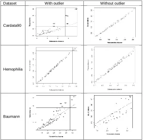
The center point has been identified in the given dataset by considering the deepness of the point through the depth values computed using projection depth and skew-adjusted projection depth under with and without outliers. The real dataset (cardata90, Champers and Hastie (1993)) has been considered for this study. The dataset consists of 60 observations with two variables, namely weight and engine displacement of cars. For each observation depth has been computed by using projection and skew-adjusted projection depth procedures. Further, the outliers in the data have been identified through distance-distance plot (Figure 1) and removed and hence computed depth values. The computed depth values for the data set under with and
without outliers are summarized in table (Table 1) and are given in appendix. The deepest point (center) is located by considering the highest depth value. It is noted from the table the skew-adjusted projection depth locates the same observation as a center (45th observation) under with and without outliers. But projection depth represents the different data points as center (17th observation and 40th observation) under with and without outliers.
3.2. Classifications Using Depth Procedures
The conventional classification procedures rely on distributional assumption such as multivariate normality and use the measures sample mean vector and covariance matrix. These measures are very sensitive to outliers. This section presents the results obtained in the context of classification problems while applying the projection and skew-adjusted projection depth procedures along with conventional and robust discriminant procedures under real and simulation environments. The efficiency of these procedures has been studied by computing average misclassification probabilities.
3.2.1 Real Data
To study the performance of the projection and skew-adjusted projection depth procedures, the two real data sets has been used for the experimental study. (i) The hemophilia data (Habemma et al. (1974)) contains two measured variables (
X
1: log10 (AHF activity) andX
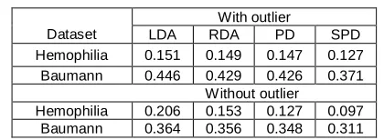
2: log10 (AHV antigen)) on 75 women, belonging to two groups, n1=30 (normal group) and n2=45 (obligatorycarries). (ii) The Baumann dataset (Moore and McCabe(1993)), consists of 66 instances, 5 variables and 3 experimental groups. The variables are pretest.1, pretest.2, post.test.1, post.test.2, post.test.3. and the three groups are basal, traditional method of teaching; DRTA, an innovative method; Strat, another innovative methodFor the given data sets, outliers are identified through distance-distance plots (Figure 1 in appendix).The computed misclassification probabilities by using depth procedures along with classical and robust discriminant procedures are displayed in the following table under with/without outliers.
Table 2: Computed misclassification probabilities under various procedures (Real Data)
Dataset
With outlier
LDA RDA PD SPD
Hemophilia 0.151 0.149 0.147 0.127 Baumann 0.446 0.429 0.426 0.371
Without outlier
3001 3.2.2. Simulation
This section presents the classification results obtained with projection, skew-adjusted projection depth procedures, and conventional, robust discriminant methods under simulating environment with/without contaminations (Location and Scale). The contaminations levels are 0%, 5%, 10%, 15%, 20%, 25%, and 30% were considered. Two cases were considered which is described below and the obtained results are displayed in the table 3.
Case 1:
To simulate the data are Three groups (g=3) with three variables (p=3) are considered. The data were generated under the normal distribution which has the covariance matrices ∑1=I3,∑2=2.5I3 and ∑3= 3I3 with means µ1= (0,0,0) ,
µ2= (3,3,3) and µ3= (5,5,5) with sample size of each group
20. The location and scale contaminations are applied as described using the values of µ1= (-4, -4,-4), µ2= (-5, -5,-5)
and µ3= (-7, -7,-7) along with the covariance matrices ∑1
=1.5I3, ∑2=4I3 and ∑3= 6I3.
Case 2:
To simulate the data are Four groups (g=4) with four variables (p= 4) are considered. The data were generated under the normal distribution which has the covariance matrices ∑1=I4 ,∑2=5I4, ∑3=7I4, and ∑4= 4I4 with means µ1=
(1,1,1,1) , µ2= (3,3,3,3) , µ3= (5,5,5,5)and µ4= (7,7,7,7) with
sample size of each group 20. The location and scale contaminations are applied as described using the values of µ1= (-3, -3,-3,-3) ,µ2= (-5, -5,-5,-5),
µ3= (-7, -7,-7,-7) and µ4= (-9, -9,-9,-9) along with the
covariance matrices ∑1 =2I4, ∑2=3I4, ∑3= 6I4 and
∑4= 8I4.
Table 3: Computed misclassification probabilities under various procedures (Simulation)
It noted from the above table, the skew-adjusted projection depth produces less misclassification probability when compared with projection depth, conventional and robust discriminant procedures. Also, it is observed that even when variable and/or group increases the skew-adjusted projection depth procedures gives better classification when compared with the other procedures. The study indicates that the skew-adjusted projection depth performs better than the other procedures. Further it is noted that the skew-adjusted projection performs well when compared with
other procedures even when the level of contamination increases.
4. CONCLUSION
The location and scatter estimator play important role for all multivariate statistical data analyses. The traditional estimates, sample mean vector and covariance matrix are most sensitive when the outlying observations in the data.. This paper explored a skew-adjusted projection depth and used it to find the good measure of location. Further the superiority of the method studied under real and simulation by applying it in discriminant analysis and by computing the misclassification probabilities over projection, conventional and robust discriminant procedures.The study concluded that the skew-adjusted projection depth gives the larger depth value over the projection depth procedures for all instances. Further, the classification results shows that it has more discriminating power over the projection, conventional and robust discriminant procedures. This procedure can be used to identify the good measure of location in a given data cloud and in turn to perform almost all kind of multivariate statistical data analyses.
REFERENCES
[1] Brys, G., Hubert, M., and Struyf, A. (2004). A robust measure of skewness. Journal of Computational and Graphical Statistics, 13, 996-1017.
[2] Brys, G., Hubert, M., and Rousseeuw, P.J. (2005). A robustification of independent component Analysis. Journal of Chemometrics, 19, 364-375. [3] Chambers, J.M. and Hastie, T.J. (1993). Statistical
Models in S, Londen: Chapman and Hall, 46-47. [4] Donoho, D. (1982). Breakdown properties of
multivariate location estimators, Ph.D. Qualifying paper, dept. Statistics, Harvard University, Boston. [5] Habemma, J.D.F., Hermans, J. and van den Broek,
K. (1974). Stepwise Discriminant Analysis Program using density estimation in Proceedings in Computational statistics, COMPSTAT (Physica Verlag, Heidelberg) ,101-110.
[6] Hubert, M. and Van Driessen, K. (2004). Fast and Robust Discriminant Analysis. Computational Statistics & Data Analysis, 45,301-320.
[7] Hubert, M., and Vandervieren, E. (2008). An adjusted boxplot for skewed distributions. Computational Statistics and Data Analysis 52, 5186-5201.
[8] Hubert, M., Rousseeuw, P.J., and Segaert, P. (2015). Multivariate Functional outlier detection. Statistical Methods and Applications, 24,177-202. [9] Liu, R.Y. (1990). On a notion of data depth based
on random simplices. The Annals of Statistics, 18, 191-219.
[10] Liu, R.Y. (1992). Data depth and multivariate rank test. In: L1- Statistical Analysis and Related Methods, 279-294. North-Holland, Amsterdam. [11] Liu, R.Y., Parelius, J.M., and Singh, K.(1999).
Multivariate analysis by data depth: Descriptive Statistics, Graphics and Inference. The Annals of Statistics, 27, 783-858.
Error
Three variables and Three groups
Four variables and Four groups
LDA RDA PD SPD LDA RDA PD SPD 0.00 0.20
7 0.17 0 0.01 4 0.07 1 0.32 5 0.26 7 0.25
3 0.237 0.05 0.25
0 0.24 6 0.21 0 0.20 7 0.41 3 0.36 0 0.33
8 0.267 0.10 0.350 0.315 0.309 0.246 0.459 0.425 0.413 0.360 0.15 0.40
0 0.36 8 0.31 5 0.27 3 0.47 5 0.45 9 0.42
5 0.425 0.20 0.42
6 0.37 0 0.36 4 0.30 9 0.60 0 0.47 5 0.45
9 0.429 0.25 0.450 0.382 0.370 0.368 0.625 0.553 0.466 0.459 0.30 0.50
0 0.42 6 0.39 3 0.37 0 0.63 7 0.56 7 0.56
3002 [12] Liu, X., and Zuo, Y. (2014). Computing projection
depth and its associated estimators. Stat.Comput. 24, 51-63.
[13] Liu, X., and Zuo, Y. (2015). CompPD: A MATLAB Package for Computing Projection depth. Journal of Statistical software 65(2), 1-21.
[14] Moore, D. S. and McCabe, G. P. (1993). Introduction to the Practice of Statistics, Second Edition. Freeman, 794–795.
[15] Rousseeuw, P.J., and Hubert, M. (1999). Regression depth. Journal of the American Statistical Association, 94, 388-433.
[16] Stahel, W. (1981). Robust Schatzungen: infinitesimal Optimalitat and Schatzungen von Kovarianzmatrizen. PhD thesis, ETH Zurich.
[17] Tukey, J.W. (1975). Mathematics and the picturing of data. In: Proceedings of the International Congress of Mathematicians, 523-531. Canadian Mathematical Congress, Montreal.
[18] Zuo, Y. (2003). Projection-based depth functions and associated medians, The Annals of Statistics, 31, 1460-1490.
[19] Zuo, Y., and Serfling, R. (2000). General notions of statistical depth function. The Annals of Statistics, 28, 461–482.
[20] Zuo, Y.J. (2006). Multidimensional trimming based on projection depth. The Annals of Statistics, 34,
2211-2251.
[21] Zuo, Y.J., and Lai, S.Y. (2011). Exact computation of bivariate projection depth and Stahel-Donoho estimator. Computational Statistics & Data Analysis, 55(3), 1173-1179.
[22] Zuo, Y.J., and Cui, H.J. (2005). Depth weighted scatter estimators. The Annals of Statistics, 33, 381-413.
[23] Zuo, Y.J., Cui, H.J., He, X.M. (2004). On the Stahel-Donoho estimators and depth – weighted means for multivariate data. The Annals of Statistics, 32(1), 189-218.
[24] Muthukrishnan, R., and Poonkuzhali, G. (2015). Computing Median with Data Depth in Multivariate Data, Journal of Modern Sciences, 7(2), 11-19. [25] Muthukrishnan, R., Gowri, D. and Ramkumar, N.
(2018).Measure of Location using Data Depth Procedures, International Journal of Scientific Research in Mathematical and Statistical Sciences ,5(6), 273-277.
[26] Muthukrishnan, R., Vadivel, M. and Ramkumar, N. (2018). Projection based Data Depth Procedure with application in Discriminant Analysis, International Journal of Research in Advent Technology, 6(5), 824-832.
[27] R Core Team, R: ―A language and environment for statistical computing‖, Vienna, Austria, 2019
APPENDIX
Figure 1: Distance-Distance Plots
Table 1: Computed Depth Values (Dataset: cardata90)
Dataset With outlier Without outlier
Cardata90
Hemophilia
3003 S. No. Weight Disp. With outlier Without outlier
PD SPD PD SPD
1 2560 97 0.373 0.385 0.330 0.379 2 2345 114 0.438 0.573 0.438 0.504 3 1845 81 0.287 0.395 0.284 0.348 4 2260 91 0.419 0.542 0.429 0.510 5 2440 113 0.495 0.650 0.523 0.697 6 2285 97 0.426 0.564 0.454 0.586 7 2275 97 0.421 0.561 0.446 0.593 8 2350 98 0.457 0.578 0.470 0.550 9 2295 109 0.422 0.570 0.422 0.510 10 1900 73 0.310 0.444 0.314 0.447 11 2390 97 0.473 0.523 0.456 0.500 12 2075 89 0.351 0.500 0.354 0.476 13 2330 109 0.438 0.604 0.446 0.565 14* 3320 305 0.099 0.160 - -
15 2885 153 0.589 0.818 0.489 0.698 16* 3310 302 0.101 0.162 - -
17 2695 133 0.685 0.834 0.753 0.864 18 2170 97 0.379 0.535 0.382 0.500 19 2710 125 0.604 0.705 0.661 0.760 20 2775 146 0.593 0.773 0.506 0.685 21 2840 107 0.284 0.323 0.276 0.332 22 2485 109 0.529 0.649 0.552 0.633 23 2670 121 0.594 0.661 0.612 0.698 24 2640 151 0.374 0.500 0.333 0.381 25 2655 133 0.641 0.804 0.658 0.749 26 3065 181 0.355 0.568 0.292 0.500 27 2750 141 0.685 0.849 0.588 0.766 28 2920 132 0.417 0.549 0.417 0.614 29 2780 133 0.647 0.839 0.697 0.874 30 2745 122 0.490 0.571 0.519 0.608 (* outlier)
31 3110 181 0.377 0.626 0.310 0.520 32 2920 146 0.659 0.874 0.657 0.852 33 2645 151 0.377 0.505 0.336 0.385 34 2575 116 0.592 0.691 0.620 0.693 35 2935 135 0.436 0.591 0.434 0.665 36 2920 122 0.330 0.406 0.329 0.434 37 2985 141 0.455 0.662 0.445 0.709 38 3265 163 0.417 0.677 0.366 0.646 39 2880 151 0.630 0.854 0.523 0.726 40 2975 153 0.712 0.879 0.592 0.776 41 3450 202 0.357 0.599 0.292 0.500 42 3145 180 0.406 0.685 0.333 0.546 43 3190 182 0.413 0.695 0.337 0.550 44* 3610 232 0.246 0.500 - -
S. No. Weight Disp. With outlier Without outlier
PD SPD PD SPD
45 2885 143 0.663 0.884 0.678 0.880 46 3480 180 0.371 0.578 0.322 0.568 47 3200 180 0.440 0.707 0.360 0.576 48 2765 151 0.481 0.646 0.416 0.539 49 3220 189 0.362 0.639 0.296 0.504 50 3480 180 0.371 0.578 0.322 0.568 51* 3325 231 0.198 0.335 - - 52* 3855 305 0.128 0.234 - - 53* 3850 302 0.131 0.240 - -
54 3195 151 0.363 0.580 0.3333 0.6040 55 3735 202 0.320 0.492 0.2915 0.5000 56 3665 182 0.287 0.500 0.2393 0.4880 57 3735 181 0.255 0.474 0.2132 0.4602 58* 3415 143 0.222 0.320 - -