Absolute risk estimation for time to event data

University of Tartu

Faculty of Science and Technology

Institute of Mathematics and Statistics

Juan Manuel Alvarado Salcedo

Absolute risk estimation for time to event data

Actuarial and Financial Engineering

Master’s Thesis (30 ECTS)

Supervisor: Krista Fischer

Absolute risk estimation for time to event data

Master’s Thesis

Juan Manuel Alvarado Salcedo

Abstract

The objective of the thesis is to use time to event models in order to estimate the absolute risk for a certain event. In particular, we will use the data from the Estonian Biobank cohort together with different approaches to estimate the Risk of Type 2 Diabetes (T2D).

We will use the methodology that accounts for right-censoring in the data. Specifically, we will use three approaches for duration models:

 Non-Parametric methods: the Kaplan-Meier estimator;

 Semiparametric model: Cox Proportional Hazard models; and

 Parametric models: models assuming Weibull and Gompertz distribution.

The analysis will be done in R software exclusively. After we have identified the optimal models, we will predict the risks, giving us an approximate estimate which will be potentially useful to personalize risk predictions for the Estonian population and insurance.

CERCS research specialisation: P160 Statistics, operations analysis, programming, financial and actuarial mathematics.

Lühikokkuvõte

Absoluutse riski hindamine elukestvusmudelitele Magistritöö

Juan Manuel Alvarado Salcedo

Magistritöö eesmärk on elukestusanalüüsi kasutades leida sobivaim meetod haiguseriskide hindamiseks. Täpsemalt kasutatakse TÜ Eesti Geenivaramu andmeid, mille põhjal soovime erinevate mudelite abil prognoosida 2. tüübi diabeedi riski. Andmed on paremalt tsenseeritud ja töös kasutatakse kolme meetodit:

 Mitte parameetriline mudel: Kaplan- Meieri meetod.

 Semiparameetriline mudel: Coxi võrdeliste riskide mudelid.

 Parameetriline mudel: mudelid Weibulli ja Gompertzi jaotuse eeldusel.

Analüüsil kasutatakse R tarkvara. Pärast mudelite loomist aitab see Eestis rahvastikul ja kindlustusfirmadel isikupõhiselt terviseriske hinnata.

CERCS teaduseriala: P160 Statistika, operatsioonianalüüs, programmeerimine, finants-ja kindlustusmatemaatika.

Table of Contents

Introduction ... 4

1. Introduction to Time to Event Models ... 5

1.1 Specific features of time to Event Data ... 5

1.2 Censoring (Fischer, 2019) ... 5

1.3 Survival Function (Collett, 2015) ... 6

1.4 Hazard Function (Collett, 2015) ... 7

1.5 Kaplan-Meier method (Collett, 2015) ... 8

1.6 Cox Proportional Hazard Model (Collett, 2015) ... 10

1.7 Parametrical Models (Collett, 2015) ... 11

1.7.1 AFT (Accelerated Failure Time) Model (Collett, 2015) ... 12

1.7.2 AFT (Accelerated Failure Time) Model Interpretation (Võrk, 2019) ... 13

1.7.3 Weibull Distribution (Collett, 2015) ... 14

1.7.4 Gompertz Distribution (Collett, 2015) ... 16

1.8 Likelihood for Censored and Uncensored data (Käärik, 2018) ... 17

2. The analysis of the Estonian Biobank Data ... 18

2.1 Overview of the Data ... 18

2.2 Data cleaning ... 19

2.3 Data Inspection ... 21

2.4 Non-Parametric approach ... 22

2.5 Models’ Interpretation ... 23

2.6 Model building (Fischer, 2019) ... 25

3. Conclusions and Recommendations ... 40

Introduction

Nowadays, one of the major directions in public health is to move towards personalized medicine, using also genomics data to improve the quality of healthcare. One important aspect of personalized medicine is personalized prediction of the risk of common chronic diseases. For that purpose, one needs to combine genomic data with conventional risk predictors to obtain new efficient risk predictors. Before those could be implemented in practice, careful validation is needed. Thus, one needs to estimate absolute risk for the disease using both conventional and new methods and assess, whether these estimates correspond to actually observed risk levels, and what is the added value of the genomic component. Statistically, methods for absolute risk prediction are needed for this kind of work. Obviously, the methods that are appropriate for time-to-event analysis are needed. As a basis for such research, data from population-based biobanks can be used.

In the present theses we first give an overview of time to event data and some basic statistical analysis methods. Currently, the most popular methods for the analysis of such data are either nonparametric or semiparametric and therefore not designed for absolute risk prediction. For latter purpose, we investigate the performance of parametric methods.

As a specific example, we consider prediction of Type 2 Diabetes risk in the Estonian Biobank Data. Type 2 Diabetes is one of the major public health problems in both developed and developing countries, leading to high healthcare costs and premature mortality due to different complications. Recently it has been shown (Läll et al 2017) that in addition to conventional risk factors (such as obesity), Poly-genic Risk Score (PGRS) may provide valuable addition to the risk prediction algorithm.

1. Introduction to Time to Event Models 1.1 Specific features of time to Event Data

Usually, time to event data is not easily analyzed by just using standard statistical methods, since we have to take into consideration events during a timeframe. It will be required to define a start point, in our case, the initial recruitment, and an endpoint, which is when the data cuts.

In addition, it is also required to use a different approach for the analysis in a mathematical sense. Typically, this data is right skewed, hence, we need to assume that the data is not normally distributed and we will have to use different a parametric approach to model the data.

Lastly, the most important feature in our analysis is that the data is censored. Broadly speaking, we will censor those alive and without Type 2 Diabetes (T2D) after the data cuts.

1.2Censoring (Fischer, 2019)

Theoretically, it is said that data is censored if by the start or endpoint of the experiment the event was not observed. In other words, the analysis will focus on those subjects that were and were not censored.

Firstly, denote:

 𝑇_𝑖 – Event Times.

 𝐶_𝑖 – Censoring Times.

We assume both are independent from each other. Then, we denote a random variable for the observed times as follows for modelling:

𝑌𝑖 = min⁡{𝑇𝑖, 𝐶𝑖}

Lastly, we define a failure indicator for 𝑖’th observation. Hence, we get:

𝛿_𝑖 = {1 𝑖𝑓⁡𝑢𝑛𝑐𝑒𝑛𝑠𝑜𝑟𝑒𝑑⁡𝑒𝑣𝑒𝑛𝑡𝑠⁡(𝐸𝑣𝑒𝑛𝑡⁡𝑂𝑏𝑠𝑒𝑟𝑣𝑒𝑑)

In time to event modelling, there are three functions of interest, since it basically helps us summarize and understand survival data. Thus, we have the survival function, the hazard function and the cumulative hazard function.

1.3Survival Function (Collett, 2015)

We can easily define it as the probability that an individual survives more than a certain time. This “time” takes a non-negative value. In other words:

𝑇 – The random variable of a lifetime of an individual.

We can now form our distribution function as follows. The probability that it does not survive till time 𝑡:

𝐹(𝑡) = 𝑃(𝑇 ≤ 𝑡) = ⁡ ∫ 𝑓(𝑥)𝑑𝑥

𝑡 0

Next, from this function we can derive the survival function, which is the probability that an individual survives till or beyond time 𝑡:

𝑆(𝑡) = 𝑃(𝑇⁡ ≥ 𝑡⁡) = 1 − 𝐹(𝑡)

There are some important properties of this survival function:

 𝑆(0) = 1, at time 0, the survivability is certain.

 𝑆(∞) = ⁡ lim

𝑡→⁡∞𝑆(𝑡) = 0, all individuals perish.

1.4Hazard Function (Collett, 2015)

The hazard function’s purpose is to express the risk of the event. In this study, T2D occurs at any time 𝑡. In actuarial terms, we can call it the force of mortality, which is the probability that an individual’s random variable 𝑇 survival time is between 𝑡 and 𝑡 + 𝜕𝑡; this is conditioned to the

fact that this 𝑇 is greater or equal to 𝑡. Denote the following:

ℎ(𝑡) – Hazard Function

ℎ(𝑡) = lim

𝜕𝑡→∞{

{𝑃(𝑡⁡≤⁡𝑇<⁡𝑡⁡+⁡𝜕𝑡⁡⁡|⁡𝑇⁡≥⁡𝑡) 𝜕𝑡 }

From this definition, there are some useful relationships with the survival functions. First, using what’s known in probability theory about conditional probability:

𝑃(𝐴|𝐵) =𝑃(𝐴, 𝐵) 𝑃(𝐵)

This leads to the following equation:

ℎ(𝑡) =𝑃(𝑡 ≤ 𝑇 < 𝑡 + 𝜕𝑡)

𝑃(𝑇 ≥ 𝑡) =

𝐹(𝑡 + 𝜕𝑡) − 𝐹(𝑡) 𝑆(𝑡)

Therefore, replacing this into the definition we get the following:

lim 𝜕𝑡→∞{ 𝐹(𝑡+𝜕𝑡)−𝐹(𝑡) 𝜕𝑡 } 1 𝑆(𝑡)

Recall the definition derivatives; in this case, it is in respect to 𝑡 and this is equal to 𝑓(𝑡)

giving us the simplified definition of the hazard function:

ℎ(𝑡) =𝑓(𝑡) 𝑆(𝑡)

It is important to say that this function itself is not a density function; we should consider it as the probability of failure or a risk event in a small period of time, given that it has survived

up till time 𝑡. Hence, the greater the hazard between times, the greater the risk of failure. Also, this definition leads to the cumulative hazard function, which will be covered later.

Below will follow a summary of non-parametric models in order to estimate the survival function. The classical approach in this study is the Kaplan-Meier method. This approach is of huge importance since it is a simplified and classical version to visualize and estimate risks.

1.5Kaplan-Meier method (Collett, 2015)

This method is usual to estimate the survival function for grouped or ungrouped censored survival analyses. In order to estimate it, we need to construct time intervals and each of the intervals is designed so that the death time is contained in the interval and taken into account just at the start of the next interval.

Next, we can suppose there are 𝑛 individuals which have different observed survival times

𝑡1, 𝑡2, … . , 𝑡𝑛. Then we assume that there are 𝑟 death times within the individuals, where 𝑟 ≤ 𝑛.

This means that there are not more death times than individuals. Consecutively, denote 𝑛_𝑗 as the number of individuals that are alive by time 𝑡𝑗 for 𝑗 = 1, 2, … , 𝑟 and denote 𝑑𝑗 as the number of

dead individuals at this time. Hence, since there are alive and dead individuals we can estimate the probability of survival through the interval as:

𝑛𝑗− ⁡ 𝑑𝑗

𝑛_𝑗

Since there are also censored survival times that occur through the intervals, this is to be taken after the death time when calculating the values of 𝑛_𝑗.

Lastly, assuming that the deaths of individuals are independent from each other, this leads to the following formula:

𝑆̂(𝑡) = ∏𝑛𝑗 − ⁡ 𝑑𝑗 𝑛_𝑗

𝑘

Some properties of this formula are:

 𝑆̂(𝑡) = 1⁡𝑓𝑜𝑟⁡𝑡 < 𝑡1⁡

 𝑛𝑟 = ⁡ 𝑑𝑟 if the largest interval observed is uncensored, and this leads to 𝑆̂(𝑡) =

0⁡𝑓𝑜𝑟⁡𝑡 ≥ ⁡ 𝑡_𝑟

 𝑛_𝑗 = 𝑛_𝑗−1− 𝑑_𝑗− 𝑐_𝑗; 𝑐_𝑗 is the censored data. Just to simplify that for each interval, we

can calculate the new individuals for each interval this way. Also, we can simplify the formula a little bit more and form the following:

⁡𝑆̂(𝑡) = ∏ (1 −𝑑𝑗 𝑛𝑗

)

𝑘

𝑗=𝑗−1

This should give us a step graph; for each step, there is a failure time.

This also leads to the hazard rate function (Võrk, 2019) estimate in a discrete way:

 𝑇 as a discrete random variable that takes values from 𝑡𝑗 < ⁡ 𝑡𝑗+1 < ⋯⁡

 Denote its probability density function:

𝑓(𝑡𝑗) = 𝑃(𝑇 = ⁡ 𝑡𝑗)

 Define the survival function, as the probability of 𝑇 is greater or equal than 𝑡_𝑗:

𝑆(𝑡_𝑗) = 𝑃(𝑇 ≥ 𝑡_𝑗) = ⁡ ∑ 𝑓(𝑡_𝑗)

∞

𝑗

 Now, define the hazard at 𝑡_𝑗:

ℎ(𝑡_𝑗) = 𝑃(𝑇 = ⁡ 𝑡_𝑗|⁡𝑇 ≥ 𝑡_𝑗) =𝑓(𝑡𝑗) 𝑆(𝑡𝑗)

The simplest way to interpret this is the ratio of survival, since it is the conditional probability of dying after surviving. From here the Kaplan’s method can also be derived.

The next model is a semi-parametric model; this is called this way because the baseline has a function that is not determined by any distribution parameters and we usually investigate how those arguments affect our hazard and those covariates are time independent.

1.6Cox Proportional Hazard Model (Collett, 2015)

Cox (1972) extended this hazard method by working on which combinations of explanatory variables affect the base hazard in order to determine the changes in time, thus, assuming the explanatory variables are constant in time.

Denote:

ℎ𝑖(𝑡) = ⁡𝜃(𝑥𝑖𝑗)ℎ0(𝑡) for 𝑖 = 1, 2, … , 𝑛

 𝑥_𝑖𝑗 is the vector of explanatory variables at the particular time of failure.

 𝜃 in our case is the function for this (𝑥_𝑖𝑗) variables, also known as relative hazard.

 ℎ_𝑖(𝑡) is our hazard function for an 𝑖’th individual at a time.

 ℎ₀(𝑡) is our base hazard function, which is usually not given.

Since our relative hazard is a non-negative function, we can express it in exp⁡(ωi̇). This is

important because we can use properties of this function like:

 ω_i̇ = ⁡ ∑ 𝛽_𝑖𝑥_𝑖𝑗

𝑛 𝑖̈=1

is the combination of explanatory variables and their values 𝛽_𝑖.

 If 𝜃(𝑥_𝑖𝑗) > 1, then the hazard of failure at a given future time 𝑡 is greater.

 If 𝜃(𝑥_𝑖𝑗) < 1, then the hazard of failure at a given future time 𝑡 is lesser.

Now that we have set up our link function, we can finally express our hazard function in a linear form and we have our regression model or proportional model as follows:

ℎ_𝑖(𝑡) = ⁡exp⁡(∑ 𝛽_𝑖𝑥_𝑖𝑗

𝑛

𝑖̈=1

From here, we can derive important relations. The most common one which we will be using is the hazard rate ratio:









e

e

e

x

x

E

x

x

E











_

_

,...,

|

1

,...,

|

In other words, the hazard ratio measures how the relative hazard rate changes if an explanatory variable changes by a unit.

The last approach that will be used is the parametric one. It is parametric because the baseline hazard follows a parametric distribution and similarly to Cox, we assume that the explanatory variables affect our response variable, hence, proportionality is also viewed.

1.7Parametrical Models (Collett, 2015)

In this chapter it is necessary to introduce the cumulative hazard function. This is easily derived from the hazard’s function idea:

ℎ(𝑡) =𝑓(𝑡) 𝑆(𝑡)

We know that:

ℎ(𝑡) = − 𝑑 𝑑𝑡𝑆(𝑡)

Hence, we can use an important derivative property; for example, there exists a 𝑔 function whose derivate is:

𝑑 𝑑𝑡log 𝑔 (𝑡) = 1 𝑔(𝑡) 𝑑 𝑑𝑡𝑔(𝑡)

Thus, from this, we get:

ℎ(𝑡) = − 𝑑

𝑑𝑡log 𝑆(𝑡) ⁡ → 𝑆(𝑡) = exp[−ℎ(𝑡)]⁡

𝐻(𝑡) = ⁡ ∫ ℎ(𝑢)𝑑𝑢 𝑡 0 → −(log 𝑆 (𝑡) − 𝑙𝑜𝑔𝑆(0)) → 𝑆(𝑡) = exp⁡(− ∫ ℎ(𝑢)𝑑𝑢 𝑡 0 ) 𝑆(0) = 𝑃(𝑇 > 0) = 1 → log(1) = 0

Using these important results, there are two important distributions that will be taken into consideration, that is, Weibull distribution and Gompertz distribution. These distributions were chosen since they are closely related to the behavior analysis of the data and are key to a proper interpretation and estimation.

1.7.1 AFT (Accelerated Failure Time) Model (Collett, 2015)

This model determines how the covariates shrink or stretch the failure time:

ℎ_𝑖(𝑡) = ⁡exp⁡(−𝜇_𝑖)ℎ₀( 𝑡 exp(𝜇_𝑖)) Where, 𝜇_𝑖 = ⁡ ∑ 𝛽_𝑖𝑥_𝑖𝑗 𝑛 𝑖̈=1

This is the linear component, similar to proportional hazards. The ℎ₀(𝑡) is given by the explanatory values when they are zero, or the intercept. Lastly, the corresponding survival function for each individual is:

𝑆_𝑖(𝑡) = ⁡ 𝑆0(

𝑡 exp(𝜇_𝑖))

Having denoted this, an important feature of this model is that they can take a log-linear representation. Thus, let us show the AFT. Consider the following random variable 𝑇_𝑖 as the lifetime of an individual in its log form:

𝑙𝑜𝑔𝑇_𝑖 = ⁡𝜇 + ∑ 𝛽_𝑖𝑥_𝑖𝑗

𝑛

𝑖̈=1

 The explanatory variables and their coefficients.

o Positive represent survival increment.

o Negative represent survival decrement.

 The 𝜇 and 𝜎 are the intercept and scale parameter.

 𝜖_𝑖⁡is the error from the linear part, with a particular probability density function (PDF).

Relating this to the survival function:

𝑆_𝑖(𝑡) = 𝑃(𝑙𝑜𝑔𝑇𝑖 ≥ 𝑙𝑜𝑔𝑡) = 𝑃 (𝜇 + ∑ 𝛽_𝑖𝑥_𝑖𝑗 𝑛 𝑖̈=1 + ⁡𝜎𝜖_𝑖 ≥ 𝑙𝑜𝑔𝑡) = 𝑃 (𝜖𝑖 ≥ ⁡ 𝑙𝑜𝑔𝑡 − ⁡𝜇 − ∑ 𝛽𝑖𝑥𝑖𝑗 𝑛 𝑖̈=1 𝜎 ⁡) = ⁡ 𝑆𝜖𝑖⁡( 𝑙𝑜𝑔𝑡 − ⁡𝜇 − ∑ 𝛽𝑖𝑥𝑖𝑗 𝑛 𝑖̈=1 𝜎 )⁡⁡

With this result we can show how the survival function of 𝑇𝑖 can be found by using the

survival function of 𝜖𝑖 and consecutively derive the accelerated failure time using different forms

of PDFs for 𝜖_𝑖. A good expression is using the percentile of the distribution of survival times.

1.7.2 AFT (Accelerated Failure Time) Model Interpretation (Võrk, 2019)

Let us briefly explain how to interpret the model with this attribute. Again, let us assume:

 𝑇_𝑖 as the lifetime of an individual in its log form.

 After some simplifications we get that:

𝑇𝑖 = exp (⁡∑ 𝛽𝑖𝑥𝑖𝑗 𝑛

𝑖̈=1

+ ⁡ 𝜖𝑖)

 If we increment a unit of our explanatory variable and divide it by the present position f

𝑇_𝑖(𝑥 + 1) 𝑇_𝑖(𝑥) = exp (⁡∑ 𝛽_𝑖(𝑥_𝑖𝑗+ 1) 𝑛 𝑖̈=1 + ⁡ 𝜖_𝑖) exp (⁡∑ 𝛽𝑖𝑥𝑖𝑗 𝑛 𝑖̈=1 + ⁡ 𝜖𝑖) = exp⁡(𝛽_𝑖)

 Hence, it has a multiplicative form and its interpretation is as follows:

 exp(𝛽_𝑖) > 1, increment in survival times.

 exp(𝛽_𝑖) < 1, decrement in survival times.

 We can also represent this in percentage:

(exp(𝛽𝑖) − 1) ∗ 100

1.7.3 Weibull Distribution (Collett, 2015)

We assume that the survival time 𝑇 has a Weibull distribution. Thus, the hazard function has the form:

ℎ(𝑡) = ⁡𝜆𝜎𝑡𝜎−1

With the survival function:

𝑆(𝑡) = exp (− ∫ 𝜆𝜎𝑢𝜎−1_𝑑𝑢 𝑡 0 ) = ⁡ exp(−⁡𝜆𝑡𝜎₎ And density: 𝑓(𝑡) = ⁡𝜆𝜎𝑡𝜎−1exp(−⁡𝜆𝑡𝜎)⁡

 ⁡𝜆 – The scale parameter or intercept.

o Reparametrizing by the regression coefficients.

 𝜎 – The shape parameter. In case of Weibull this is calculated by the inverse of the

esti-mate:

o 1

𝛾= ⁡𝜎

o 𝛾 = 1, hazard is constant, replace this distribution by the exponential distribution.

o 𝛾 < 1, hazard decreases over time. Properties:

 The AFT is a unique measure associated with survival time.

 If the shape parameter is constant, then we can go from AFT to proportional hazards

(PH) and vice versa.

 With this knowledge, we will use the AFT property of this model for interpretation.

Let us briefly show the calculation for the parameters for AFT in this model:

ℎ_𝑖(𝑡) = ⁡ 𝜆_𝑖ℎ₀(𝑡), 𝜆_𝑖 = ⁡ ∑ 𝛽_𝑖𝑥_𝑖𝑗

𝑛 𝑖̈=1

and ℎ₀(𝑡) = 𝜎𝑡𝜎−1

Recall (1) and replace:

𝑙𝑜𝑔𝑇𝑖 = ⁡𝜇 + ∑ 𝛽𝑖𝑥𝑖𝑗 𝑛

𝑖̈=1

+ ⁡𝜎𝜖𝑖⁡, with 𝜇 = − log 𝜆 and 𝜎, after some calculations we get:

𝑙𝑜𝑔𝑇_𝑖 = ⁡𝜎 ∑ 𝛽_𝑖𝑥_𝑖𝑗

𝑛

𝑖̈=1

+ 𝛽₀+ ⁡𝜎𝜖_𝑖, ⁡𝛽₀ = ⁡ − log 𝜆

 The 𝜖𝑖 follows Gumbel’s PDF. Using it we can derive the survival function and also

the cumulative hazard.

Another way to solve for 𝜆_𝑖 is using the relation of PH and AFT if the shape is constant:

𝜆_𝑖 = exp (−

∑ 𝛽_𝑖𝑥_𝑖𝑗

𝑛 𝑖̈=1

𝜎 )

Weibull’s parameters estimated in R by the function “Survreg” in the library “survival” are usually given in AFT for direct interpretation after exponentiating them.

1.7.4 Gompertz Distribution (Collett, 2015)

If the survival time 𝑇 has a Gompertz distribution, the hazard function has form:

ℎ(𝑡) = ⁡𝜆exp⁡(𝛾𝑡)

With survival function:

𝑆(𝑡) = exp (− ∫ 𝜆 exp(𝛾𝑢) 𝑑𝑢 𝑡 0 ) = exp {⁡𝜆 𝛾[1 − exp(−⁡𝜆𝑡 𝛾_)]} And density: 𝑓(𝑡) = 𝜆exp⁡(𝛾𝑡)exp {⁡𝜆 𝛾[1 − exp(−⁡𝜆𝑡 𝛾_)]}⁡

 𝜆 is the scale parameter.

 𝛾 the shape parameter:

o 𝛾 > 1, hazard increases over time.

o 𝛾 = 1, hazard is constant, replace this distribution by the exponential distribution.

o 𝛾 < 1, hazard decreases over time.

Parametrization comes immediately from proportional hazards:

ℎ(𝑡) = exp (∑ 𝛽𝑖𝑥𝑖𝑗 𝑛 𝑖̈=1 ) ℎ0(𝑡) where ℎ0(𝑡) = ⁡𝜆exp⁡(𝛾𝑡) Properties:  PH interpretation.

 It is widely used for demographic purposes and it was introduced for human mortality

modelling.

 It does not have an AFT interpretation. However, it is significantly more accurate in

1.8Likelihood for Censored and Uncensored data (Käärik, 2018)

This section is to show the derivation of the likelihood function to understand the fitting process for censored and uncensored data.

Recalling the definition of censored and uncensored data, we have:

𝑌_𝑖 = min⁡{𝑇_𝑖, 𝐶_𝑖} and 𝛿_𝑖

Hence, combining both terms we get:

(𝑌_𝑖, 𝛿_𝑖)

Since we spoke about independence of both censoring time and event time, we can consider for censored data (𝛿𝑖 = 0):

𝑃(𝐶_𝑖 = 𝑡, 𝑇_𝑖 > 𝑡) = 𝑃(𝐶_𝑖 = 𝑡)𝑃(𝑇_𝑖 > 𝑡) = ⁡ 𝑓_𝐶𝑖(𝑡)𝑆_𝑇𝑖(𝑡)⁡

Similarly, if (𝛿_𝑖 = 1) or for uncensored data:

𝑃(𝐶_𝑖 > 𝑡, 𝑇_𝑖 = 𝑡) = 𝑃(𝐶_𝑖 > 𝑡)𝑃(𝑇_𝑖 = 𝑡) = ⁡ 𝑓_𝑇𝑖(𝑡)𝑆𝐶𝑖(𝑡)⁡

Therefore, applying both results, the likelihood can be denoted as:

∏{𝑓𝑇𝑖(𝑡𝑖)𝑆𝐶𝑖(𝑡𝑖)}𝛿𝑖{𝑓𝐶𝑖(𝑡𝑖)𝑆𝑇𝑖(𝑡𝑖)}1−𝛿𝑖⁡⁡ 𝑛

𝑖=1

From here, it is easy to derive parameter estimates for either Gompertz or Weibull distributions.

2. The analysis of the Estonian Biobank Data 2.1Overview of the Data

The database used in this thesis includes the following variables:

 47832 observations.

 "bmi": Body Mass Index.

 "fruit", "fveg": scores for consuming fresh fruit and fresh vegetables (1: never, 2: 1 – 2 d/week, 3: 3 – 5 d/week, 4: 6 – 7 d/week).

 "smoke": smoking level.

 "educ": education (important for classification: >3: secondary; >5: university).

 "pa": a physical activity score (combining exercise and walking activities, the score

indicates the decile the individual belongs to).

 "recr.date", "end.date" : date of recruitment/end of follow-up (or death).

 "dead": whether the person has died.

 "T2D": Type 2 Diabetes diagnosis in the database.

 "T2D.date": date of T2D diagnosis.

 "pgrs": the polygenic score (scaled combination of the effects of 7500 genetic

markers).

The analysis was done with R software 1due to its versatility and visual pack-ages. It is imperative to reinstate the research purpose and develop the analysis based on these questions:

 What is the risk How risky is for an individual to get T2D at a given time?

 How do our explanatory variables modify this risk?

 Can we use a model to predict individualized risk for T2D? What is the proportion

of people to be at risk at a given time? Based on the model, are we able to stratify individ-uals to categories with different risk level?

 How do predicted risk categories differ in terms of the actually observed risk level

(proportion of diagnoses observed in 5 years) in these categories?

2.2Data cleaning

Before starting the analysis and variable selection, some modifications were made to the data frame, such as:

 Removing those that got T2D before the recruitment time.

 Leaving out individuals who are younger than 30 or older than 80, to have a more

homogeneous sample.

 Creating the time scale variable by:

o Defining a variable corresponding to the “end” date: the date of T2D diagnosis for those who got the diagnosis during follow-up; the date of death for those who did not get the T2D diagnosis, but died before the end of follow-up time (before May 16th_{, 2019) and the date of the end of follow-up (May 16}th_{, 2019)}

for the rest.

o Then defining the variable for the follow-up time by subtracting the recruitment date from the end date and dividing by 365.25.

o An event indicator was defined to have value 1 for those who got T2D diagnosis before the end of follow-up and 0 for others.

 Selection of variables. The ones which we will use in this research are the following:

o BMI: it is the physical condition that we can modify and manipulate, and it affects different medical conditions, including T2D.

o PGRS: the main variable of our research. Those with a higher number are prone to live shorter lives. Numerically, it is a continuous variable.

 Standardizing the PGRS variable, to make it with mean 0 and standard deviation of 1,

thus making it easy to manipulate and interpret.

 Categorizing the BMI into quantiles for three groups, for future interpretations:

Group 1: [14.48, 22.66) - (lowest 20% of the BMI distribution)

o Group 2: [22.66, 30.86) - (individuals between 20% and 80% quantiles)

o Group 3: [30.86, 60.10] - (highest 20% of the BMI distribution)

 Categorizing the PGRS into quantiles for into three groups, for future interpretations:

o Group 1: [-3.852, -0.84) - (lowest 20% of the PGRS distribution)

o Group 2: [-0.84, 0.843) - (individuals between 20% and 80% quantiles)

o Group 3: [0.843, 4.033] - (highest 20% of the PGRS distribution) In case of future modifications, these will be explained during the analysis.

2.3Data Inspection

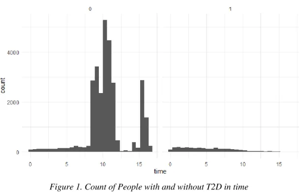
After carrying out these modifications, we are left with 31614 observations. Part of the data familiarization is conducting simple visual inspections; there are 2659 people with T2D and 28955 without diabetes.

In the graph, 0 means censored, or no diabetes and 1 is that the event happened.

From figure 1, the count of people with “1” T2D and without “0” during time is notable. giving a small visual about the time at which people are more at risk of getting T2D.

2.4Non-Parametric approach

Estimating the Kaplan method using the time variable, with the function “Surv” in R soft-ware, shows the following:

Figure 2. Illustration of R, censoring effect.

Those times with “+” sign mean that they were censored and those without it mean that an event happened at that time. If we wished to get a summary for our Kaplan, it is possible to apply the function “survfit”, thus getting the following:

Figure 3. Estimation survival function.

It can be calculated manually in the following way:

𝐼𝑓⁡𝑡 = 5 → 𝑆̂(5) = ∏𝑛𝑗 − ⁡ 𝑑𝑗 𝑛𝑗 = 𝑆(0) ∗ ⁡𝑛2 − ⁡ 𝑑2 𝑛2 =29098 − 1401 29098 ≈ 0.95⁡⁡ 2 𝑗=1 𝑛₂ = 𝑛₁− 𝑐₁− 𝑑₁ = 31614 − 2516 − ⁡0 = 29098

Visually, in figure 4 we can see the survival estimate plot against time:

Figure 4. A plot of the Kaplan-Meier estimate of the Survival function.

Figure 5. A plot of the Kaplan-Meier estimate of the failure time distribution function.

Likewise, in the figure 5. the failure time distribution can be estimated, using the method shown above. This method does not take into account the explanatory variables; however, it does give a nice approach to estimate the risk level in the population is at a given time and it provides the foundations for viewing the survival probability of not getting T2D.

2.5Models’ Interpretation

Before we begin building our main model, it is common to establish the foundations by using a simple model and interpret those variables of interest. This will give us an insight into how the explanatory variables behave. For this, we will use Weibull’s AFT property and Gompertz’s PH property. Using the function of “survreg” and the Weibull distribution, we get the parameter estimates that shown in the Table 1:

Table 1. Weibull’s coefficients estimates.

Variable Coefficients exp(coefficients) se(coefficients) z p PGRS -0.333 0.717 0.0215 -15.46 <2e-16

AGE -0.038 0.962 0.0017 -21.70 <2e-16 BMI -0.132 0.876 0.0039 -33.92 <2e-16

According to our first table. All our variables make significant changes towards our event, and the interpretation follows easily from Weibull, since by using this package we can directly interpret the AFT just by exponentiating them.

 A unit increase in the genetical score means a decrement the time to diabetes times

by 28.3%.

 Aging by one year means a decrement in times to diabetes times by 3.8%

When time passes and with this combination of variables, they do have a negative effect on surviving T2D.

Next, we want to build the proportional hazard’s model. Although we can use Weibull’s property, we will use Gompertz model due to its immediate interpretation from the coefficients.

Using the function of “flexsurvreg” in R, then specifying the distribution and lastly adding the combination of variables, we get the following:

Table 2. Gompertz coefficient estimates

Variable Coefficients exp(coefficients) se(coefficients )

PGRS 0.309 1.363 0.0192

AGE 0.036 1.036 0.0015

BMI 0.123 1.131 0.0029

In the second table, although it does not specify the p-value, we can still assume from Weibull’s model that they are significant. The coefficients are given in the form of PH, so we can directly interpret them by exponentiating them:

 Incrementing a unit of the genetical score means a hazard increment by a factor of

1.363 or 36.3% in time.

 Aging by one year means a hazard increment by a factor of 1.036 or 3.6% in time.

 Incrementing a unit of the BMI means a hazard increment by a factor of 1.131 or 13.1%

in time.

In other words, in time, the hazard will increase if we increase any of these variables, thus, making the Estonian population more susceptible to getting T2D.

Having understood the effect of our main variables, we would like to create a model that is good to predict risks in categories, in order to understand the number of people in this data that are at risk.

2.6Model building (Fischer, 2019)

The model building process takes time and it could be a never-ending loop, so we should always find a balance and provide a good model conserving our variables of interest. In the fol-lowing we will show the different steps and techniques which will help us to assess and provide a model for risk predictions. We will begin by separating our data set into two parts. Given the size of the data set, we get:

 The first data set consisting of 15000 observations; we will use this one for model

development.

 The second data set consisting of 16614 observations; we will use this one for

validat-ing.

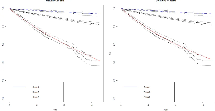
We plot both survival curves by using the distributions as well as the Kaplan-Meier estimates, comparing our already categorized BMI and PGRS. This visual inspection helps to understand the fit of our distributions.

Figure 6. Weibull and Gompertz Distribution survival plot for BMI categories.

After using both categories, in figure 6 and figure 7, we can observe that both distri-butions are good at predicting, as the predicted survival curve mostly falls between the confidence intervals of the Kaplan-Meier Estimate. This poses another question: which distribution is the best? In order to answer this, we can develop two proportional risk tables, in order to know the number of people that fall between each risk category. The process is as follows:

 Developing two new models that include all variables of interest without categories

and distributions of interest, so the predictions will be based on the testing variables.

 Estimating the 5-year risk for each individual using our models from the testing

data set.

 Creating a data frame using these risk predictions from our validation data frame.

 Calibrating the observed and predicted numbers of each category.

 Comparing and seeing if there are discrepancies.

Table 3. Weibull’s Observed Count Risk Estimates – 5 Years

Risk Estimate Classification

Count of People with T2D (0,0.01] 7 (0.01,0.02] 42 (0.02,0.03] 60 (0.03,0.04] 81 (0.04,0.05] 75 (0.05,0.07] 131 (0.07,0.10] 127 (0.10,1] 217

Table 4. Weibull’s predicted count Risk Estimates – 5 Years

Risk Estimate Classification Count of People with T2D (0,0.01] 16.37 (0.01,0.02] 59.30 (0.02,0.03] 68.94 (0.03,0.04] 65.81 (0.04,0.05] 59.26 (0.05,0.07] 98.90 (0.07,0.10] 109.58 (0.10,1] 225.92

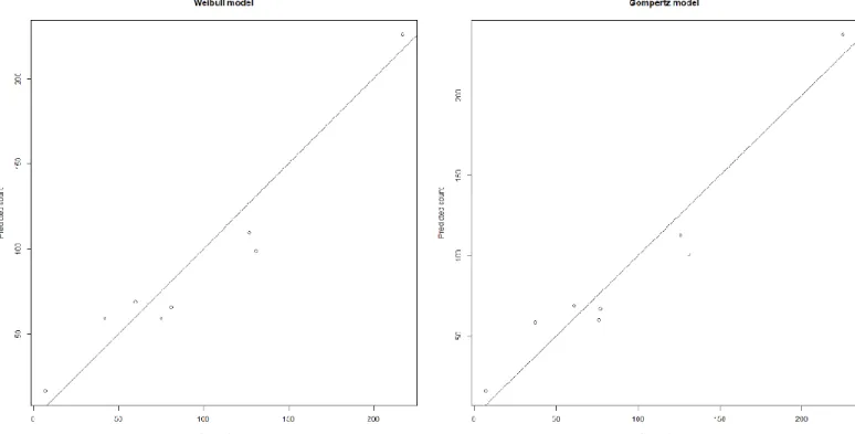
When comparing both predicted tables 4 and 6 and observed tables 3 and 5 for Weibull and Gompertz, they are not so far from each other; it is a good indication that both distributions are good choices. Next, we do a calibration plot of the observed versus predicted values. This will provide a visual insight into whether there are differences within both distributions.

Table 6. Gompertz’s predicted count Risk Estimates – 5 Years

Risk Estimate Classification Count of People with T2D (0,0.01] 15.59 (0.01,0.02] 58.51 (0.02,0.03] 68.80 (0.03,0.04] 67.14 (0.04,0.05] 60.00 (0.05,0.07] 100.82 (0.07,0.10] 112.84 (0.10,1] 237.75

Table 5. Gompertz’s Observed Count Risk Estimates – 5 Years

Risk Estimate Classification Count of People with T2D (0,0.01] 7 (0.01,0.02] 37 (0.02,0.03] 61 (0.03,0.04] 77 (0.04,0.05] 76 (0.05,0.07] 131 (0.07,0.10] 126 (0.10,1] 225

The plots in figure 8 illustrate the non-existing differences between both Gompertz and Weibull. Now let us compare the predicted proportions versus the observed proportions, which should lead to the same conclusion:

If we want to grade the goodness of fit of our models, we can perform a Chi-square Test to determine:

 Ho: the predictions are not different from the observed.

 Ha: the predictions are different from the observed.

 However, the results specify rejection of the null hypothesis:

Weibull: 32.80, degrees of freedom: 7. Gompertz: 30.50, degrees of freedom: 7.

We still have to work the discrepancies in our predictions. However, given the results, we can proceed with the Weibull distribution, due to its simplicity and versatility.

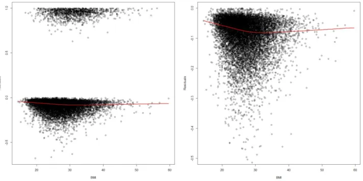
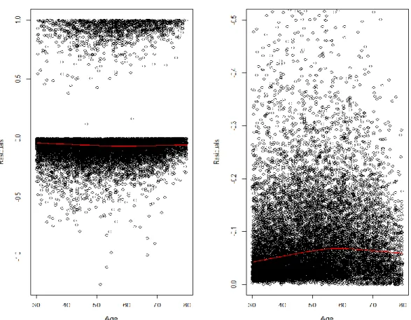
Now, let us improve the model. The next step is to go through our variables; we want to know whether the BMI and age need transformations or regrouping. This follows the non-linearity and non-proportionality assumption. We can see this by plotting the Martingale residuals.

This can be performed by using a Cox model (T, 2015), since if a Weibull model is valid, then, Cox model (as a proportional hazards model) should also be valid. Hence, we can start by creating a model with age + PGRS. Then, by plotting the residuals against the BMI, we get the following:

This plot suggests that the effect of BMI could be different for those with BMI < 30 and those with BMI > 30. Therefore, we can split this variable into two groups:

 BMI1: if BMI < 30; then it is equal to BMI, otherwise BMI1 = 30.

 BMI2: if BMI > 30, BMI2 = BMI-30. Otherwise BMI2 = 0. This way we can

pre-vent duplication and analyze this effect individually.

The BMI variable in total is equal to the sum of those groups, hence, the interpretation for BMI2 should be additive to BMI1. Thus, we get the following:

Table 7. Cox model coefficient estimates

Variables Coefficients exp(coefficients) se(coefficients) z p PGRS 0.330166 1.391199 0.028508 11.58 <2e-16

AGE 0.033852 1.034432 0.002329 14.54 <2e-16 BMI1 0.193469 1.213452 0.013174 14.69 <2e-16 BMI2 0.106903 1.112826 0.008040 13.30 <2e-16

We clearly see in table 7 that there is a different significant effect on BMI2, so it is advis-able to leave this variadvis-able split before we begin our interpretation for this model. We also want to know if age needs to be changed. In order to do this, we will use the combination of PGRS + BMI1 + BMI2 and plot the residuals against Age.

This plot also suggests that the effect of Age could be different for those with Age < 60 and those with Age > 60. Therefore, we can split this variable into two groups:

Age1: if Age < 60; then it is equal to Age, otherwise Age1 = 60.

Age2: if Age > 60, Age2= Age - 60. Otherwise Age2 = 0., so that we can analyze the additional years’ effect individually and prevent duplications.

Table 8. Cox model coefficient estimates

Variables Coefficients exp(coefficients) se(coefficients) z p BMI1 0.188475 1.207407 0.013220 14.257 <2e-16 BMI2 0.105366 1.111118 0.008051 13.088 <2e-16 Age1 0.049191 1.050421 0.004027 12.215 <2e-16 Age2 0.004462 1.004472 0.006712 0.665 0.506 PGRS 0.327731 1.387815 0.028440 11.524 <2e-16

We see in the table 8 that the additive effect of Age2 is not significant; hence, we can take it out of the model. This means that we only care about those until Age 60 for good predictive power and less bias.

Now that we have set our important variables, we can plug this into our parametric Weibull model together with some other variables, just to improve the predictive power. These are:

 Smoke: SM1: Current and SM2: Former.

Table 9. Weibull’s coefficients estimates.

Variables Coefficients Std. Error z p

(Intercept) 13.42779 0.52544 25.56 < 2e-16 BMI1 -0.20340 0.01531 -13.29 < 2e-16 BMI2 -0.11338 0.00917 -12.37 < 2e-16 Age1 -0.05504 0.00420 -13.12 < 2e-16 PGRS -0.34753 0.03209 -10.83 < 2e-16 Ed1 0.28924 0.07724 3.74 0.00018 Ed2 0.27171 0.08472 3.21 0.00134 SM1 -0.37027 0.07636 -4.85 1.2e-06 SM2 -0.22222 0.08310 -2.67 0.00749

According to this model, just by reading the signs in the table 9’s coefficients, those with education tend to increase their survival times, this might be related to the fact that with higher education indicates nutrition knowledge, and those that currently smoke have a greater effect on decreasing their survival times versus those that used to smoke or never smoked. Another important aspect to notice is that former smokers have a less significant effect on getting the T2D; however, given the predictive power, we will keep this variable.

This leads to the initial question of whether our model will perform better with this variable selection. Let us do our risk table and compare it with the old model:

Table 10. Risk Estimate Classification for Old model. Risk Estimate

Classification

Count of people with T2D Predicted count of people with T2D Predicted proportion of people with T2D (0,0.01] 7 16.36709 0.003147482 (0.01,0.02] 42 59.29812 0.010427011 (0.02,0.03] 60 68.94806 0.021574973 (0.03,0.04] 81 65.80843 0.042676502 (0.04,0.05] 75 59.26187 0.056646526 (0.05,0.07] 131 98.90059 0.078302451 (0.07,0.1] 127 109.58021 0.096285064 (0.1,1] 217 225.92218 0.158741770

Table 11. Risk Estimate Classification for New model.

Risk Estimate Classification

Count of people with T2D Predicted count of people with T2D Predicted proportion of people with T2D (0,0.01] 12 21.35478 0.003326864 (0.01,0.02] 45 48.56960 0.013574661 (0.02,0.03] 63 54.55964 0.028636364 (0.03,0.04] 62 57.07445 0.037758831 (0.04,0.05] 51 51.37999 0.044425087 (0.05,0.07] 109 93.30552 0.069162437 (0.07,0.1] 132 112.71170 0.097705403 (0.1,1] 266 286.42160 0.149859155

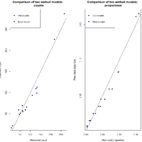
We see that the new model’s count in the table 11 is closer to the real count versus the old model in the table 10. Let us plot and test by Chi-square to see if there are any differences.

It is visible in the figure 12 that the new model is better in counts and proportion, except when predicting the higher risk classification; yet, we see by the Chi-square goodness of fit that:

 Old model: 32.80, degrees of freedom: 7.

 New model: 13.50, degrees of freedom: 7.

Thus, improving the model.

Let us explore another method to assess our model accuracy called NRI or Net Reclassification Index (Inoue, 2018). This index provides the proportions of individuals for whom prediction was improved using different sets of explanatory variables. It is important to consider that it is a probability measure but not a proportion.

In our case, let us compare whether adding PGRS improves our reclassification to test this method:

Table 12. Net Reclassification Index Whether PGRS improves or not the classification.

Estimate Lower Upper

NRI 0.09419059 0.04200935 0.14402763

We see in the table 12 estimate that by adding this variable it makes an impact on reclassifying those individuals. Hence, it is important to keep this variable in our model. Let us compare our complex model with our basic model and see whether the complex model’s predictions are better.

Table 13. Net Reclassification Index. Whether complex model improves or not the classification.

Estimate Lower Upper

NRI 0.18484306 0.13835307 0.23448185

It is visible in the table 13 estimate that the complex model helps reclassifying the individuals in their categories, making it much better in prediction. Hence, this model is good enough to keep it.

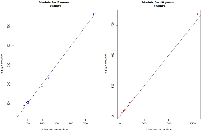
With the complex model that we have just created we can perform the risk estimation for 5 and 10 years.

Table 14. Risk Estimates for the complex model for 5 Years. Risk Estimate Classification Observed Count of people with T2D Predicted count of people with T2D (0,0.01] 27 39 (0.01,0.02] 76 90 (0.02,0.03] 97 104 (0.03,0.04] 100 108 (0.04,0.05] 104 100 (0.05,0.07] 202 187 (0.07,0.1] 244 231 (0.1,1] 551 553

Note: With Chi-square: 8.981407, df = 7

Table 15. Risk Estimates for the complex model for 10 Years. Risk Estimate

Classification

Observed count of peo-ple with T2D Predicted count of people with T2D (0,0.01] 14 17 (0.01,0.02] 39 65 (0.02,0.03] 73 86 (0.03,0.04] 79 98 (0.04,0.05] 89 105 (0.05,0.07] 197 222 (0.07,0.1] 304 303 (0.1,1] 1590 1672

+

We can see in the figure 13 and table 14 that at 5 years the differences are not significant compared to the observed counts and it is also visible that our Chi’s estimate that it has a good fit. However, when estimating for 10 years, the difference between predicted counts and observed counts is significatively large. Our calibration plot shows good fit, just at the end of the model in 10 years there is a discrepancy with the highest classification. However, adjusting this with reality and following the world trends, approximately 9% of the population suffers from T2D.2 We can say that it over predicts the number of people at risk within their categories, usually companies always try to mitigate any possible outcome and we can interpret this over prediction as beneficial.

2 _{https://www.statista.com/statistics/271464/percentage-of-diabetics-worldwide/}

3. Conclusions and Recommendations

With the present work we have explored the performance of different nonparametric, semiparametric and parametric methods to estimate the risk of Type 2 Diabetes in the Estonian Biobank data.

When analyzing, we have used the Kaplan-Meier method to view how the survival curve and the failure curve look in given time scale. We have also used this basic approach to estimate the probability of surviving T2D and illustrate the effect of time on our data set. This is very important in order to establish the beginning of our research.

We have shown that for this data, both Weibull and Gompertz model perform equally well. Therefore, the use of Weibull model is acceptable in this context, as it is simple and has both proportional hazards and accelerated failure time interpretations. In our model-building and validation process we used separate independent datasets for model-building and validation of the final risk estimates. We have found that the risk estimates found by Weibull model perform reasonably well, allowing us to stratify individuals to different risk categories, where the model-predicted risk level is similar to the observed risk level in the data.

We have also found that the genetic score (PGRS) improved the model significantly, with almost 10% more people being reclassified to correct categories than incorrect ones. In future, the model could be developed further by allowing for competing risk (by mortality) and possible additional covariates. Developing a significant model with the capability of being updated by any sort of change or research.

4. References

Collett, D. (2015). Modelling Survival Data in Medical Research. Boca Raton: CRC Press. Fischer, K. (2019, September). Statistical analysis of follow-up data in large biobank cohorts.

Tartu, Tartumaa, Estonia.

Gillespie, B. (2006). Checking Assumptions in the Cox Proportional Hazards Regression Model. Dearborn, Michigan, United States of America.

Inoue, E. (2018). nricens: NRI for Risk Prediction Models with Time to Event and Binary. R package version 1.6. https://CRAN.R-project.org/package=nricens.

Jackson, C. (2016). flexsurv: A Platform for Parametric Survival Modeling in R. Journal of Statistical Software, 1-33.

Käärik, M. (2018, Fall). Survival Models. Tartu, Tartumaa, Estonia: University of Tartu.

Kenneth, H. (2019). muhaz: Hazard Function Estimation in Survival Analysis. R package version 1.2.6.1. https://CRAN.R-project.org/package=muhaz.

Kiefer, N. M. (1988). Economic Duration Data and Hazard Functions (Vol. 26). Journal of Economics Literature.

Lancaster, T. (1990). The Econometric Analysis of Transition Data. Cambridge: Cambridge University Press.

Müller, H. W. (2020). dplyr: A Grammar of Data Manipulation. R package version 0.8.4. https://CRAN.R-project.org/package=dplyr.

T., T. (2015). A Package for Survival Analysis. version 2.38. https://CRAN.R-project.org/package=survival.

Non-exclusive licence to reproduce thesis

I, Juan Manuel Alvarado Salcedo

1. Herewith grant the University of Tartu a free permit (non-exclusive licence) to

reproduce, for the purpose of preservation, including for adding to the DSpace digital archives until the expiry of the term of copyright,

Absolute risk estimation for time to event data. supervised by Krista Fischer.

2. I grant the University of Tartu a permit to make the work specified in p. 1 available to the public via the web environment of the University of Tartu, including via the DSpace digital archives, under the Creative Commons licence CC BY NC ND 3.0, which allows, by giving appropriate credit to the author, to reproduce, distribute the work and communicate it to the public, and prohibits the creation of derivative works and any commercial use of the work until the expiry of the term of copyright.

3. I am aware of the fact that the author retains the rights specified in p. 1 and 2.

4. I certify that granting the non-exclusive licence does not infringe other persons’ intellectual property rights or rights arising from the personal data protection legislation.

Juan Manuel Alvarado Salcedo