Multivariate linear mixed models for statistical genetics

(1)

Multivariate linear mixed models

for statistical genetics

Francesco Paolo Casale

European Bioinformatics Institute

Hughes Hall College

University of Cambridge

This dissertation is submitted for the degree of

Doctor of Philosophy

(2)

(3)

Declaration of Originality

This dissertation is the result of my own work and includes nothing which is the outcome of work done in collaboration except as declared in the Preface and specified in the text. It is not substantially the same as any that I have submitted, or, is being con-currently submitted for a degree or diploma or other qualification at the University of Cambridge or any other University or similar institution except as declared in the Pref-ace and specified in the text. I further state that no substantial part of my dissertation has already been submitted, or, is being concurrently submitted for any such degree, diploma or other qualification at the University of Cambridge or any other University of similar institution except as declared in the Preface and specified in the text.

This dissertation does not exceed the specified length limit of 60,000 words as defined by the Biology Degree Committee.

(4)

(5)

Abstract

In the last decade, genome-wide association studies have helped to advance our under-standing of the genetic architecture of many important traits, including diseases. How-ever, the statistical analysis of genotype-phenotype associations remains challenging due to multiple factors. First, many traits have polygenic architectures, which means that they are controlled by a large number of variants with small individual effects. Second, as increasingly deep phenotype data are being generated there is a need for multivariate analysis approaches to leverage multiple related phenotypes while retain-ing computational efficiency. Additionally, genetic analyses are confronted by strong confounding factors that can create spurious associations when not properly accounted for in the statistical model. We here derive more flexible methods that allow integrat-ing genetic effects across variants and multiple quantitative traits. To do so, we build on the classical linear mixed model (LMM), a widely adopted framework for genetic studies.

The first contribution of this thesis is mtSet, an efficient mixed-model approach that enables genome-wide association testing between sets of genetic variants and multiple traits while accounting for confounding factors. In both simulations and real-data applications we demonstrate that mtSet effectively combines the advantages of variant-set and multi-trait analyses.

Next, we present a new model for gene-context interactions that builds on mtSet. The proposed interaction set test (iSet) yields increased statistical power for detecting polygenic interactions. Additionally, iSet enables the identification of genetic loci that are associated with different configurations of causal variants across contexts. After benchmarking the proposed method using simulated data, we consider two applications to real datasets, where we investigate genetic effects on gene expression across different cellular contexts and sex-specific genetic effects on lipid levels.

Finally, we describe LIMIX, a software framework for the flexible implementation of different LMMs. Most of the models considered in this thesis, including mtSet and iSet, are implemented and available in LIMIX. A unique aspect of the software is an inference framework that allows a large class of genetic models to be defined and, in many cases, to be efficiently fitted by exploiting specific algebraic properties. We demonstrate the utility of this software suite in two applied collaboration projects.

Taken together, this thesis demonstrates the value of flexible and integrative mod-elling in genetics and contributes new statistical methods for genetic analysis. These approaches generalise previous models, yet retain the computational efficiency that is needed to tackle large genetic datasets.

(6)

(7)

Acknowledgments

First and foremost, I would like to thank my supervisor Oliver Stegle for being a superb advisor and mentor. His enthusiastic guidance, feedback and support have been invaluable to me, for the work in this thesis and beyond.

I am thankful to EMBL-EBI and the University of Cambridge for providing an excellent and stimulating environment to perform my research. I would also like to thank my advisory committee. A special thank goes to my internal advisor John Marioni for all the stimulating discussions and his continuous presence and support, thanks also to Jan Korbel and Carl Rasmussen for the precious feedback on my work. A big thank also to Ewan Birney for his scientific advice and support.

I am grateful to the whole Stegle group for all the insightful discussions, their feed-back and the time together. A special thank goes to the people I had the opportunity to work more closely with: Barbara Rakitsch, Amelie Baud, Rachel Moore and Danilo Horta.

Thanks to the numerous proofreaders of this thesis: Rachel Moore, Davis McCarthy, Hannah Meyer, Nils Koelling, Amelie Baud, Myrto Kostadima, Verena Zuber, Danilo Horta, Tommaso Leonardi, Barbara Rakitsch, Leland Taylor and Na Cai.

Being in Cambridge and at the EBI has been marvellous, I feel lucky and proud to have been part of these communities, of course for the science, but not only that. Many people have contributed to make this experience astonishingly pleasant and rich in so many ways. In particular, thanks to Michele, Myrto, Nils, Mitra, Angela, Ernest, Ana, Maria, Steve, Konrad and Joana for the fantastic time together. A special thank also to Salvatore, Martina and Danilo.

I am grateful to my parents Raffaele and Emma and my brother Ivo for their unconditional love and support. Thanks also to Francesco and Andrea for their love and belief. Last but not least, I would like to thank Federica for being so supportive and patient along these years. There are no words to describe how lucky I feel to have such an exceptional partner in life.

(8)

(9)

1 |

Introduction

The main contributions of this thesis are in the field of statistical genetics. Statistical genetics is concerned with the development and the application of statistical methods to study genetic variation and inheritance in living organisms. In this chapter, I give an overview of this field and the necessary background for the work in this thesis. After discussing genetic variation and its patterns in human in Section 1.1, I give an overview of models and methods to study genetic effects on phenotypes in Section 1.2. In Section 1.3, I discuss some of the statistical challenges in modern genetics. Finally, Section 1.4 concludes this chapter with an outline of the thesis structure and the main contributions.

1.1 Genetic variation

In this section I discuss the mechanisms of genetic variation and inheritance.

1.1.1 DNA and genetic variants

All the information needed to build and sustain an organism is encoded in its genome. The genome is organised into chromosomes, which consist of long molecules of de-oxyribonucleic acid (DNA) (Brosius, 2009) and other elements. In chromosomes, DNA is composed of two strands, which are sequences of smaller molecules called nucleotides (Alberts et al., 2014). Each nucleotide in the sequence contains one of four distinct bases (adenine - A, thymine - T, guanine - G or cytosine - C). The two strands are kept together by hydrogen bonds between opposite bases. As these bonds can form only between specific pairs of bases (G with C and A with T) the two sequences are complementary. The number, length and shape of chromosomes differ between species. The human genome consists of 23 pairs of chromosomes: 22 pairs of non-identical copies of autosomal chromosomes (one inherited from the father and the other from the mother) and one pair of sex chromosomes. Females have two non-identical copies

(14)

of the X chromosome (one from each of the two parents), while males have only one copy of the X chromosome (from the mother) and one copy of the Y chromosome (from the father). The two non-identical copies of a chromosome are called homologous.

The human genome consists of approximately 3 billion base pairs (bp) (Venter et al., 2001; Lander et al., 2001). Pairs of individuals share on average 99.5% of the DNA sequence (Levy et al., 2007). A change in the sequence across individuals in a population is commonly referred to as a genetic variant while the different forms of the sequence are called alleles. An individual’s collection of alleles at a genetic locus (i.e., at a location in the genome) is referred to as the genotype of that individual. An individual is homozygous at a genetic locus on an autosomal chromosome if it has two copies of the same allele; otherwise it is heterozygous at the locus. Depending on the length and type of the sequence variation we can distinguish two types of genetic variants: single nucleotide polymorphisms and structural variants (Frazer et al., 2009). Single nucleotide polymorphisms (SNPs) are substitutions of a single base pair and are the most common type of genetic variation. Most SNPs are bi-allelic, meaning that only two possible alleles are observed in the population (International HapMap Consortium, 2005). Structural variants are changes that involve more than a single base pair and include short insertions and deletions (collectively referred to as indels) as well as larger variants at the chromosome scale, including duplications, deletions, inversions and insertions.

1.1.2 The biological process underlying inheritance

Meiosis is the process of cell division that leads to the formation of sperm cells in males and egg cells in females, collectively called gametes. In contrast to somatic cells, which have two copies of each chromosome (diploid), gametes only have one copy of each chromosome (haploid). The union of a sperm and an egg cell generates a diploid cell, the zygote, which is the first cell of a new organism.

Meiosis starts with the pairing of homologous chromosomes in a diploid cell. Each chromosome is then duplicated giving rise to a pair of chromatids. At the end of this process each chromosome has four homologous chromatids. Identical and non-identical copies of homologous chromatids are called respectively sister and non-sister chromatids. At this stage non-sister chromatids may exchange segments of genetic material, an event that is known as a crossover. Finally, through two rounds of cell di-vision the cell gives rise to four gametes. Each gamete randomly receives one of the four homologous chromatids from each chromosome. This selection occurs independently for each chromosome, leading to a mixture of maternal and paternal chromosomes in

(15)

each gamete. An important consequence of crossovers is that gametes may contain chromosomes that are a mixture of the two grandparental chromosomes from the same parent. During the process of fertilisation a sperm and an egg fuse to generate the zygote. Each zygote inherits approximately 1/4 of the genetic material from each of the grandparents. The processes of meiosis and fertilisation are shown inFig. 1.1.

eggs zygote sperm FATHER MOTHER meiosis fertilisation

crossovers I division II division

DNA replication

Figure 1.1: Meiosis and fertilisation. The figure illustrates key stages of the pro-cesses of meiosis and fertilisation, for simplicity considering a single chromosome.

Crossovers are random events and the rate of their occurrence depends on many factors, including sex, chromosome location, temperature and age. The occurrence of a crossover in a region reduces the likelihood of a new crossover in proximity. In every meiotic event, on average approximately 55 crossovers occur in males and 82 in females (Laird and Lange, 2010). The number of crossovers taking place between two loci is not an observable quantity. However, if genotype data are available one can sometimes infer whether a recombination event between two loci has occurred (Morgan, 1915; Laird and Lange, 2010). Note that the occurrence of a recombination only gives information about whether an odd or an even number of crossovers has taken place between the two loci. If at least one crossover between two loci has occurred then the fraction of gametes with a recombination is 50%. The rate of recombination between two loci can thus be estimated as θ = (1₋P0)/2 (Mather, 1938), where P0 is the

probability of no crossover. For loci that are extremely close on the same chromosome we haveP0 ≈1and θ≈0. These loci tend to be inherited together and are therefore

(16)

in linkage. Conversely, for loci that are far apart on the chromosome we have P0 ≈0

andθ= 1. In linkage studies, recombination rates have been used to infer the distance between loci on chromosomes and thus generate genetic maps (see Section 1.2.2).

1.1.3 Human genetic variation

Allele frequency is an important property of genetic variants. The frequency of an allele at a genetic variant is the proportion of chromosomes in the population that carry that allele (Laird and Lange, 2010). For a bi-allelic variant, the frequency of the less common allele (minor allele) is called the minor allele frequency (MAF). For multi-allelic variants, the MAF typically indicates the frequency of the second most common allele.

Based on their MAF, genetic variants are classified as either common or rare, where commonly a cut-off of 1% is used to define rare variants (MAF<1%) and common vari-ants (MAF>1%) (Frazer et al., 2009). Comparative analyses of genomic sequences have provided evidence for over ten millions of common variants (Frazer et al., 2009). Importantly, allele frequencies of common variants vary widely across groups of indi-viduals from different geographical regions, with many common variants segregating across populations. This phenomenon is known as population structure and is the con-sequence of non-random mating primarily due to geographical distance. In contrast to common variants, rare variants are unnumbered and include variants that are specific to close relatives or single individuals (Frazer et al., 2009).

Another central concept in genetic variation is linkage disequilibrium (LD). Two loci are in LD if some combinations of their alleles tend to occur together more of less often than expected by chance. There are different factors that determine LD between variants, including genetic linkage (see above), selection and population struc-ture (Slatkin, 2008). Different measures of LD have been proposed over the years (for a review see Devlin and Risch, 1995). A widely used measure of LD is the squared Pearson correlation between the minor allele counts in the population (Benner et al., 2016; Pickrell et al., 2016; Yang et al., 2012).

The sequencing of the first human genome (Venter et al., 2001; Lander et al., 2001) was followed by the start of the HapMap Project (Gibbs et al., 2003) that aimed at characterising patterns of human genetic variation in different populations with a focus on common variants. This international effort genotyped more than 10 million SNPs in 270 individuals from four human populations (Nigerians, Europeans, Chinese and Japanese). One fundamental result of this study was the haploblock structure of the human genome: the human genome is characterised by regions in which

(17)

recombina-tion events are limited, resulting in haplotype blocks1 characterised by high LD within them. Notably, 550,000 haplotype blocks in Europeans and Asians and 1,100,000 hap-lotype blocks in Africans were sufficient to accurately summarise the genetic variation described by common SNPs with MAF > 5% (International HapMap Consortium, 2005). An important implication of this finding is that sparse genotype data at tagging SNPs are sufficient to reconstruct most of the genome-wide genetic variation of com-mon variants, an insight that is key to the success of genome-wide association studies (see Section 1.2.3) and genotype imputation (Howie et al., 2009; Marchini and Howie, 2010).

Exploiting the higher coverage at reduced costs offered by next-generation sequenc-ing (NGS) technologies (Metzker, 2010), the 1000 Genomes Project aimed at studysequenc-ing high-coverage sequences of at least 1,000 individuals from different world-wide pop-ulations (1000 Genomes Project Consortium, 2010). In three phases, the consortium generated reference maps of human genetic variation, first considering 1,092 individuals form 14 populations (1000 Genomes Project Consortium, 2012) to finally characterise the genetic variation between 2,504 individuals from 26 human populations. In addition to characterising SNPs and short indels (up to 500 bp, 1000 Genomes Project Consor-tium, 2015), the 1000 Genomes project has also progressed the boundaries of detecting and genotyping structural variants (1000 Genomes Project Consortium, 2015). Col-lectively, the results from the project provide “the most comprehensive view of global human variation so far” (Birney and Soranzo, 2015).

1.2 From genetic variation to phenotype

Understanding how genetic variation affects phenotypes is a long standing goal in bi-ology. In this thesis, I will interchangeably use the terms "phenotype" and "trait" to indicate any measurable feature of an individual, which can be a disease state as well as a molecular or cellular feature. Additionally, I will refer to loci that are associated with a trait as a quantitative trait locus (QTL) for that trait. In this section, I give a brief historical overview of the approaches that have been used to study genetic effects on traits.

1.2.1 The first genetic models

Many consider Mendel’s work “Experiments in plant hybridisation” the beginning of sta-tistical genetics (Mendel, 1866). Studying inheritance of dichotomous traits in plants,

(18)

Mendel discovered the existence of a dominant and a recessive form of a trait. Anal-ysis of phenotype data in successive generations led Mendel to formulate the law of segregation: “One allele of each parent is randomly and independently selected, with probability 1/2, for transmission to the offspring; the alleles unite randomly to form the offspring’s genotype” (Laird and Lange, 2010).

In parallel to Mendel’s work, Francis Galton, fascinated by Darwin’s book “On the Origin of Species” (1859), studied inheritance of height and intelligence in human (Gal-ton, 1869). The traits considered by Galton seemed to follow completely different laws of inheritance from those described in Mendel’s work: the parental forms of these traits appeared somehow to be mixed in the offspring. Such traits that do not follow Mendelian patterns of inheritance are commonly referred to as complex traits.

This paradox was solved in 1918 by the theoretical work of the statistician Ronald Fisher (Fisher, 1918). Fisher showed that an additive genetic model with a large num-ber of small-effect loci results in a continuous normally distributed trait. Moreover, he proved that the phenotypic correlation between individuals is proportional to the quantity of genetic material they share. This result demonstrated that heritable com-plex traits are affected by many genes, each following Mendel’s principle of inheritance. A few decades later, building on Fisher’s work, Charles Henderson derived the solution of the mixed model equation (Henderson, 1950). Nowadays linear mixed models con-stitute the standard tool for many genetic analyses and are the basic building block of this thesis.

1.2.2 Linkage analysis

Genetic studies were initially performed solely using phenotype data. In the beginning of the 20th century, the development of the first genotyping technologies introduced the possibility to identify the genomic position of genetic markers and disease genes, giving rise to a branch of statistical genetics known as gene mapping. The first statistical method used for gene mapping was linkage analysis. The core idea underlying this approach is to use the realised recombination rate between pairs of loci in a short pedigree to infer relative genomic distances and build linkage maps (see Griffiths, 2005, chap 5). The same methodology has been successfully applied to locate disease variants for many Mendelian traits by using genotype and phenotype data on pedigrees over one/two generations. The strategy employed to map disease loci is to test for linkage between any of the genotyped markers and the disease variant (whose genotype is inferred from the phenotype data) by testing whether the recombination rate between the two loci is significantly different from 1/2 (θ ₆= 1

(19)

short pedigrees is that only a few recombinations can occur between loci in linkage so that sparse marker information (up to hundreds of markers per chromosome) are sufficient to map disease variants, although with limited resolution. Examples for some of the first linkage analyses include Alzheimer’s disease (Schellenberg et al., 1991), cystic fibrosis (Lathrop et al., 1988) and Huntington’s disease (Gusella, 1984). However, the method has been less successful in mapping genes for complex disorders (Altmüller et al., 2001).

1.2.3 Genome-wide association studies

High-throughput genotyping technologies, including SNP arrays and low-coverage se-quencing, have enabled genotyping of hundred of thousands to millions of common SNPs in increasing sample sizes. These technological advances, together with the find-ings from the Hapmap project on the haploblock structure of the human genome (see Section 1.1.3) laid the foundation for the success of genome-wide association stud-ies (GWAS, Frazer et al., 2009), currently the most widely used design for gene map-ping (McCarthy et al., 2008). GWAS rely on the LD between genotyped and causal variants, which are potentially not typed, to identify loci implicated in traits and dis-eases. Contrarily to linkage studies, GWAS are commonly performed in populations of unrelated individuals (Astle and Balding, 2009), enabling the analysis of larger sample sizes (typically from 1,000 to 100,000 individuals or even larger2). The basic principle underlying GWAS is to test for association between individual genotyped variants and the trait of interest. Given the large number of genome-wide variants to be tested, stringent criteria of significance are needed to control the number of false discoveries at the expense of statistical power (see Section 2.2.1).

The first GWAS in human was published in 2005 and revealed two genetic loci associated with age-related macular degeneration (Klein et al., 2005). Ever since, GWAS have become increasingly popular, yielding important insights into the genetic architecture of many complex traits, including type 2 diabetes (Scott et al., 2007), inflammatory bowel disease (Khor et al., 2011) and major depression (Kohli et al., 2011; Cai et al., 2015). Today, the GWAS Catalog (Burdett et al., 2015) includes more than 2,500 published GWA studies and more than 24,000 SNP-trait associations (August 2016).

Importantly, dense genotype data, such as those from the HapMap, the 1000 Genomes project and, more recently, the UK10K population (Huang et al., 2015) can

2

Consortia such as UK Biobank (Sudlow et al., 2015) have currently been producing and studying cohorts of 500,000 individuals.

(20)

be used as a reference for imputing genotypes at unobserved loci, thereby completing sparse genotype data (Howie et al., 2009; Marchini and Howie, 2010). Recent GWA studies in cohorts with NGS genotype data have attempted to identify effects from rare variants (UK10K Consortium, 2015). However, the robust identification of rare-variant effects remains challenging, as it requires extremely large sample sizes (Risch and Merikangas, 1996; Bush and Moore, 2012).

1.2.4 Molecular mechanisms from genotype to phenotype

In the process of gene expression, the genetic information stored in the DNA is used to produce molecular products. The information on the composition of these products is contained in restricted portions of the genome known as genes. In the first step of gene-expression (transcription), genes are transcribed into ribonucleic acid (RNA) molecules. Although RNA molecules can be the final product of gene expression, many RNA molecules are translated into proteins in a process known as translation. Proteins are long chains of smaller molecules called amino acids. Only approximately 1.5% of the human genome codes for proteins (Lander et al., 2001) while a large fraction of the remaining portion is likely to play a role in the regulation of gene expression (ENCODE Project Consortium, 2004). The impact of genetic variation on phenotypes is the consequence of perturbations to this complex molecular machinery.

An easily interpretable mechanism through which genetic variants may affect phe-notype is the direct alteration of the structure of the coded protein and thus of its functionality. For example, sickle cell anaemia is caused by a SNP in the HBB gene, which causes a substitution of an amino acid in the sequence of the coded protein (Laird and Lange, 2010). Alternatively, genetic variation may affect the regulation of gene expression. One way this can occur is through the disruption of a specific sequence that affects the binding of proteins regulating the expression of a gene. Another possi-bility is the alteration of the structure of the DNA, thereby affecting the functionality of regulatory elements and ultimately gene expression (ENCODE Project Consortium, 2004; Kundaje et al., 2015). Importantly, these structural changes are not necessarily associated with a change in the DNA sequence and are collectively referred to as epi-genetics, where the prefixepi-is from Greek and means "outside of" (Spector, 2012). Importantly, such changes can be "inherited" in the process of cellular division and play a key role in regulation of gene expression. Examples of epigenetic modifications are DNA methylation and histone modifications. Specifically, DNA methylation is the process through which a hydrogen atom in adenine or cytosine is replaced by a methyl group. Methylation of promoters (i.e., the DNA sequences where transcription is

(21)

initi-ated) is associated with the silencing of the corresponding gene (Alberts et al., 2014). Another important class of epigenetic changes are modifications of structural proteins, known as histones, which play a key role in the packing of DNA in chromosomes. No-tably, histone proteins can undergo more than 100 histone modifications (Ernst and Kellis, 2010), which can be reversibly written and erased by specific enzymes. The com-bination of the different histone modifications determines “the histone code” (Alberts et al., 2014). Different combinations have been associated with transcribed regions, enhancers, promoters, and other functional regions (Ernst and Kellis, 2010). Regula-tory elements can lie far from the regulated gene (Alberts et al., 2014), hampering the identification of genes underlying known GWAS loci.

DNA RNA _{global traits}

and disease regulatory elements proteins GWAS pQTL mapping eQTL mapping hQTL, mQTL, ... mapping EWAS

Figure 1.2: Overview of genetic analysis of molecular and global traits. Shown are different molecular layers and association analyses that can be considered to link ge-netic variation to different molecular and global traits. The grey arrow shows the most likely causal direction of these effects. Of course there are numerous exceptions to this simplified scheme. Regulatory elements include DNA methylation, histone modifica-tion, binding affinity for different proteins, etc. hQTL, mQTL, eQTL, pQTS mapping stand for histone modification, methylation, expression and protein QTL mapping. In order to map genes whose regulation is associated with phenotypic changes, many studies have considered genome-wide association testing between epigenetic features and complex traits, including disease, mainly focusing on DNA methylation (Paul and Beck, 2014). These studies are known as epigenome-wide association studies (EWAS).

The decrease in cost of high-throughput profiling of gene expression has made it possible to measure gene expression levels in large numbers of individuals, thereby enabling the mapping of quantitative trait loci for gene expression (eQTL mapping, Schadt et al., 2003). More recently, these studies have been extended to test for genetic effects on different regulatory elements, including DNA methylation (Gaunt et al., 2016), histone modifications (Grubert et al., 2015) as well as the activity of known

(22)

proteins and protein complexes that regulate expression and chromatin accessibility, such as transcription factors (Waszak et al., 2015). An overview of the different genetic analyses and their relationship to GWAS is given inFig. 1.2.

As genetic effects on molecular traits may depend on factors such as tissue, en-vironment and cell type, it is necessary to measure expression and other molecular traits in disparate cellular contexts. For this reason, the Genotype-Tissue Expression Project (GTEx Consortium, 2015) has been collecting and analysing gene expression profiles for more than 50 tissue types from over 900 donors.

Molecular QTL mapping entails QTL mapping for tens of thousands of molecu-lar measurements. Therefore the “small sample size/high number of tests” problem in these analyses is even more severe than in GWAS. Moreover, genetic analysis of molec-ular traits are typically performed in datasets with smaller sample sizes compared to GWAS3. To circumvent this issue, many studies have focused on mapping proximal (putativelycis-acting) QTLs by restricting association testing to genetic variants that are close to the analysed molecular trait as they are more likely to have an effect on the molecular phenotype compared to distal genetic variants.

1.3 Statistical challenges in genetics

Despite ever increasing sample sizes, the statistical analysis of genetic data remains challenging. In this section I discuss the limitations of the standard GWAS approach and recent extensions focusing on aspects that are relevant to the contributions of this thesis.

Polygenic architectures. A main limitation of the GWAS methodology is that many complex traits have highly polygenic architectures with numerous weak-effect variants (Frazer et al., 2009). This is one potential source of “missing heritability” (Ma-her, 2008), where heritability is defined as the fraction of phenotypic variance explained by additive genetic effects. This narrow-sense definition of heritability does not include dominance effects and genetic interactions, which are included in the definition of broad-sense heritability (Visscher et al., 2008). Heritability was traditionally estimated from phenotype data on pedigrees (see Falconer and Mackay, 1996), for example by re-gressing the parental average trait against the trait in the offspring (Laird and Lange, 2010). The phenomenon of “missing heritability” refers to the positive difference be-tween these heritability estimates and the proportion of phenotypic variance explained

(23)

by the additive effects of GWAS loci. Performing GWAS in increasingly large cohorts has helped recover some of this missing heritability, by revealing new associated loci for traits such as height (Wood et al., 2014), intelligence (Rietveld et al., 2013) and schizophrenia (Ripke et al., 2014). An alternative approach is to jointly model the effects from multiple genetic variants. This strategy has been shown to recover large proportions of the missing heritability for many complex traits (Yang et al., 2010; Lee et al., 2012b; Gusev et al., 2014; Eichler et al., 2010). A widely used approach to aggregate genetic effects across multiple variants is to use a random effect within a linear mixed model (LMM), the same approach initially proposed by Fisher to model inheritance of complex traits (Fisher, 1918). Prior to applications in human studies and following Fisher and Henderson’s work, LMMs had been extensively used in the field of animal breeding (Fisher, 1921; Fisher and Mackenzie, 1923; Henderson, 1984). Recent studies have shown that genetic effects are not uniformly distributed along the genome (Gusev et al., 2013) and that genetic loci can harbour multiple causal variants (Wood et al., 2011; Chiba-Falek et al., 2012; Trynka et al., 2011; Ehret et al., 2012; Patsopoulos et al., 2013; Corradin et al., 2014). These findings have motivated the development of set tests, a class of models that allows joint testing of multiple variants in genetic regions (Wu et al., 2011; Listgarten et al., 2013; Brown et al., 2016). Set tests have been shown to improve genetic mapping over single-variant approaches, recovering parts of the unexplained genetic variance (Wu et al., 2010; Listgarten et al., 2013; Brown et al., 2016).

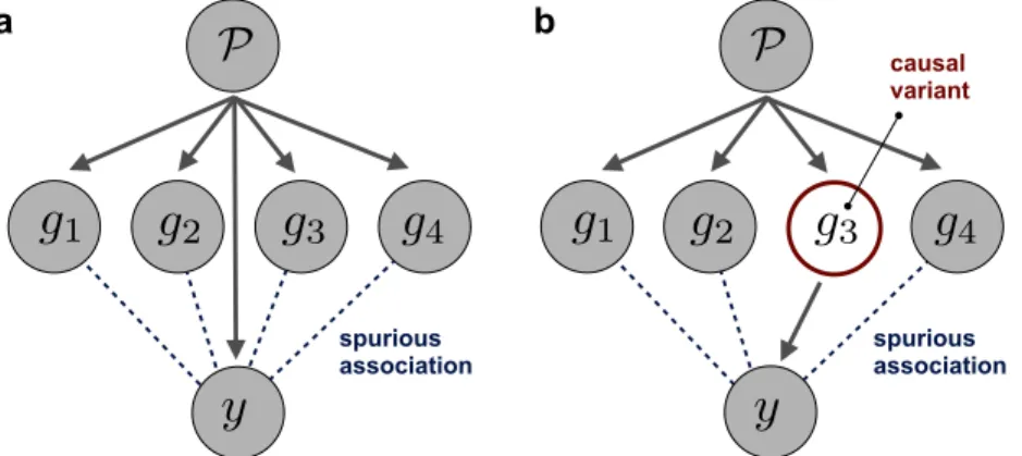
Correcting for confounding. A second challenge in GWAS is confounding factors, which can lead to spurious genotype-trait associations (McClellan and King, 2010; Lam-bert and Black, 2012; Pritchard et al., 2000b; Patterson et al., 2006). A well-studied confounder in association studies is population structure (Marchini et al., 2004). To showcase its action, let us suppose we have a population dataset consisting of individ-uals from different ethnic groups. As alleles at many different loci tend to co-occur in individuals from the same ethnic group, the genotype data will be characterised by genome-wide LD between variants. As shown inFig. 1.3a, if we consider a quantitative trait that is also influenced by ethnicity (for example because it is affected by an envi-ronmental factor determined by the geographic region of origin), a GWAS will retrieve many spurious genetic associations (see Lander and Schork, 1994). In this example, population structure exhibits a shared influence on both phenotype and genotype data. As shown inFig. 1.3b, population structure can also cause genuine genetic signal from causal variants to be mirrored in numerous non-causal loci in LD (Ewens and Spielman,

(24)

1995). Similar problems affect genetic analyses of related individuals, where genome-wide genetic similarities are correlated with environmental factors, thereby creating many spurious genotype-trait associations (Eu-Ahsunthornwattana et al., 2014).

As discussed in further detail in the next chapter, several methods have been pro-posed to correct for such confounding factors. Among these different strategies, the linear mixed model has emerged as a particularly robust approach as it can handle different types of confounding, including complex population structure and related-ness (Kang et al., 2008b; Kang et al., 2010). However, fitting LMMs can be generally computationally demanding. Although recent computational advances have enabled application of specific LMMs to genetic analyses in large cohorts (Kang et al., 2008b; Zhou and Stephens, 2012; Kang et al., 2010; Lippert et al., 2014a), the application of more complex LMMs is challenging due to a large computational burden.

a b

P

g

1

g

2

g

4

y

g

3

P

g

1

g

2

g

4

y

g

3 causal variant spurious association spurious association

Figure 1.3: Two causal networks of confounding. Population structure (_P) affects genome-wide genotypes, creating long-range LD between variants. In (a)_P also affects the trait of interest (y), a scenario that creates spurious associations in GWAS. In (b)

P does not have an effect on the trait, however, because of long-range LD, the effect of the causal genotype g3 can be mirrored at physically distant loci in an association

test.

Multivariate analysis of related phenotypes. As increasingly deep phenotype data are becoming available in human cohorts, there has been a growing interest in multivariate analyses. Multivariate models have several benefits. First, many complex traits and diseases are affected by shared genetic and environmental influences (Fortune et al., 2015; Frazer et al., 2009). For example, Pickrell et al. (2016) found that a notable proportion of the variants affecting age at menarche also affect height (36%), age of voice drop (30%), BMI (28%), breast size (10%) and male pattern baldness (10%).

(25)

The phenomenon of a variant affecting multiple traits is also known as pleiotropy and its occurrence in human traits is pervasive (Sivakumaran et al., 2011). Joint genetic analyses of multiple traits have been shown to increase statistical power by leveraging trait-to-trait correlations induced by shared genetic and environmental factors (Korte et al., 2012; Zhou and Stephens, 2014). Second, genetic effects on phenotypes can depend on environment, sex, age and other contextual variables (Dick, 2011; Winkler et al., 2015; Sasaki et al., 2015; Kang et al., 2014). By modelling the same trait in varying contexts, multivariate approaches can help characterising the context-specific architecture of genetic effects (Korte et al., 2012; Kang et al., 2014). Beyond the analysis of global phenotypes, these multivariate approaches are also important to characterise the genetic regulation of molecular traits across tissues (Price et al., 2011; Sul et al., 2013), environments (Smith and Kruglyak, 2008), development (Francesconi and Lehner, 2014) and external stimuli (Fairfax et al., 2014). Finally, multivariate analyses can be used to investigate the molecular mechanism of genetic effects by enabling joint analyses across multiple phenotypic and molecular layers (Wallace et al., 2012; Pickrell et al., 2016; Giambartolomei et al., 2014). Despite these benefits, many multivariate models are hampered by poor computational scalability, hindering their application to larger cohorts. For example, variant-set tests across multiple traits were limited to analyses of small cohorts prior to the work presented in this thesis. Additionally, the number of possible integrative analyses grows dramatically with the dimensionality of the phenotypic data.

1.4 Thesis overview and individual contributions

The challenges described in Section 1.3 illustrate the limitations of the “one-variant-to-one-trait” approach of standard GWAS and highlight the need for novel integrative methods. The linear mixed model has emerged as a flexible framework for many genetic analyses. Linear mixed models ensure robust control of confounding effects and have been widely used for association testing for single-variants (Kang et al., 2008b; Zhou and Stephens, 2012; Sikorska et al., 2013) and variant-sets (Listgarten et al., 2013; Lippert et al., 2014a). Moreover, recent computational advances have enabled efficient single-variant association tests across multiple traits (Zhou and Stephens, 2014; Lippert et al., 2014b; Furlotte and Eskin, 2015). Despite these developments, two main factors have limited application of a larger class of LMMs to genetic analyses. First, with the exception of some particular cases, LMMs are generally computationally inefficient. Second, available software are designed to perform very specific analyses while

(26)

frame-works that enable the flexible design of genetic models are not widely available (an exception is Gilmour et al., 2009). In this thesis, I present novel and efficient LMMs that can model relationships between multiple variants and traits, and describe an inference framework that enables LMMs to be built flexibly.

In Chapter 2, I give an overview of current LMMs for genetic analyses, covering their use for association testing, heritability estimation, variance decomposition, set tests and multi-trait modelling.

In Chapter 3 I present an extension of existing LMM inference schemes that enables association testing between multiple variants and traits in large cohorts (mtSet). After demonstrating and benchmarking the model in extensive simulations, I discuss two applications to real data. This work was done in collaboration with Barbara Rakitsch, Christoph Lippert and Oliver Stegle and resulted in the following publication

• Francesco Paolo Casale?, Barbara Rakitsch?, Christoph Lippert, and Oliver Ste-gle. “Efficient set tests for the genetic analysis of correlated traits.” Nature methods 12, no. 8 (2015): 755-758.

? _{Joint first authorship}

Individual contributions:

Francesco Paolo Casale and Barbara Rakitsch developed the method. Francesco Paolo Casale and Barbara Rakitsch analysed the data. Christoph Lippert pro-vided analysis tools and contributed to the interpretation of results.

Building on the mtSet framework, in Chapter 4, I derive novel tests for interactions between variant-sets and categorical contexts (iSet). iSet can be used for interaction testing either in (i) datasets where trait measurements are available in the same set of individuals in different contexts or (ii) by stratifying a population into distinct sub-groups based on an external context variable. In extensive simulations, I demonstrate that iSet offers power advantages compared to previous interaction tests. Additionally, the model can identify regions associated with changes in the configuration of causal variants across the analysed contexts. I discuss results from applications of iSet to a monocyte stimulus eQTL study (Fairfax et al., 2014) and a gene-by-sex interaction analysis of blood lipid traits. The work was done in collaboration with Danilo Horta, Barbara Rakitsch and Oliver Stegle and resulted in the following publication

(27)

“Joint genetic analysis using variant sets reveals polygenic gene-context inter-actions.” PLoS genetics 13.4 (2017): e1006693.

Francesco Paolo Casale developed the method and analysed the data. Barbara Rakitsch and Danilo Horta provided analysis tools.

In Chapter 5 I present LIMIX, a mixed-model framework that allows performing dif-ferent genetic analyses in one tool. LIMIX has been used in several projects to conduct variance component analyses (Dubin et al., 2015a; Sasaki et al., 2015; Baud et al., 2017; Chen et al., 2016), single- and multi-trait association test (Kawakatsu et al., 2016; Horton et al., 2016; Sudmant et al., 2015; Schor et al., 2017; Cannavò et al., 2016) and genomic predictions (Märtens et al., 2016). The advantage of LIMIX over other tools is its flexibility, which allows designing customised models to best suit the scope and data of specific studies. All the models considered in this thesis are im-plemented within the LIMIX software framework, including both new methods and a wide range of existing approaches that were used for comparison. Finally, to show-case the importance of flexible modelling to investigate high dimensional data I present two applied analyses from collaborative projects. The first analysis is part of a col-laborative project with Jacob Degner, Ignacio Shor, Oliver Stegle Ewan Birney and Eileen Furlong’s group at EMBL in Heidelberg, Germany (see Schor et al., 2017). The aim of this project is to understand the impact of genetic variation on transcription initiation in Drosophila melanogaster during development. The second analysis is a component of the BluePrint-WP10 project (Chen et al., 2016) and done in collabo-ration with Lu Chen, Oliver Stegle, Nicole Soranzo and others. In this analysis, we leverage high-resolution genetic, epigenetic and transcriptomic data in three human immune cell types (I will show results only from one cell type in this thesis) to quantify the contribution ofcis-genetic andcis-epigenetic effects to gene expression variability.

• LIMIX framework.

Francesco Paolo Casale, Danilo Horta and Barbara Rakitsch wrote the source code for flexible inference. Francesco Paolo Casale wrote the source code for the set tests and the variance decomposition module. Christoph Lippert and Oliver Stegle wrote the source code for fixed effect testing.

• QTL mapping of transcription initiation in Drosophila development.

(28)

Francesco Paolo Casale, Jacob Degner and Oliver Stegle designed the statistical models. Jacob Degner and Francesco Paolo Casale performed the QTL map-ping. Igacio Shor, Jacob Degner, Eileen Furlong and Oliver Stegle interpreted the results.

• Dissecting genetics and epigenetics effects in three immune cell types.

Francesco Paolo Casale, Oliver Stegle and Nicole Soranzo designed the statistical models. Francesco Paolo Casale performed the analysis. Nicole Soranzo, Oliver Stegle and Francesco Paolo Casale interpreted the results.

Finally, in Chapter 6, I give a summary of the work in this thesis and provide an outlook on future research.

(29)

2 |

Linear mixed models for genetic

analyses

The linear mixed model (LMM) has become the standard framework for many genetic analyses. LMMs provide robust control for confounding factors, allow for aggregating genetic effects from multiple variants and enable the joint analysis of multiple traits. While inference in LMMs is in general computationally demanding, efficient implemen-tations of specific LMMs enable applications to large datasets. In this chapter, I give an overview of the use of LMMs in genetics and efficient algorithmic implementations. In Sections 2.1-2.2, I discuss linear models and basic concepts of genome-wide associ-ation studies (GWAS). In Section 2.3, I introduce the LMM and discuss applicassoci-ations in genetics. Finally, in Section 2.4, I present the extension of LMMs to the analysis of multiple traits.

2.1 Linear regression

A linear model describes a continuous output variable as a linear function of one or more input variables (also referred to as features). Denoting with N the number of samples, yi the output variable for sample i and {xi1, . . . , xiF} F input variables for

sample i, the linear model can be cast as

yi = F X f=1 xifβf +ψi, withψi ∼ N 0, σe2 . (2.1)

The residual termψiaccounts for the fact that thex-yrelationship is not deterministic

because of measurement noise or other unmodelled factors. ψi is here assumed to

follow a normal distribution with mean0and varianceσ2

e and to be independent across

samples, i.e. cov(ψi, ψj) = 0. In equation (2.1), βf denotes the weight of the input

(30)

Introducing the output vector y, the input matrix X, the weight vector β and the residual vectorψ as y=       y1 y2 .. . yN      , X =       x11 x12 . . . x1F x21 x22 . . . x2F .. . ... . .. ... xN1 . . . xN F      , β=       β1 β2 .. . βF       and ψ =       ψ1 ψ2 .. . ψN      , (2.2) the linear model in (2.1) can be expressed in matrix form as

y=Xβ+ψ, withψ _{∼ N} 0, σ2_eIN

, (2.3)

whereIN denotes the N ×N identity matrix.

2.1.1 Maximum likelihood solution

Equation (2.3) specifies the probability distribution of the data p y|X,β, σ2

e

given the input variablesX and the model parametersβ andσ2

e. This probability is known

as the likelihood of the model and, for parameter inference, is typically regarded as a function of the model parameters and denoted as _L β, σ2

e

. The model in (2.3) can thus be equivalently specified as

L β, σ2_e=p y|X,β, σ_e2=N y|Xβ, σ2_eIN , (2.4) or more directly as y_{∼ N} Xβ, σ_e2IN . (2.5)

The log marginal likelihood of the model can be explicitly expressed as

log_L β, σ2 e =₋N 2 log (2π)− 1 2Nlogσ 2 e− 1 2σ2 e (y₋Xβ)>(y₋Xβ). (2.6) The maximum likelihood estimator (MLE) of the model parameters is defined as the set of parameter values that maximise the likelihood (or its log). Denoting withβˆ and ˆ

σ2

e the MLE ofβ and σ2e we can write

ˆ β,σˆ2_e =argmax_β_,σ2 e L β, σ 2 e . (2.7)

(31)

The MLE ofβandσ2

e can be found by equating the gradients of the log likelihood to 0 ∂logL β, σ2 e ∂β ! β= ˆβ,σ2 e=ˆσ2e = 0 (2.8) ∂logL β, σ2 e ∂σ2 e ! β= ˆβ,σ2 e=ˆσ2e = 0 (2.9)

From these two equations it can be easily shown that

ˆ β = X>X−1X>y (2.10) ˆ σ_e2 = 1 N y₋Xβˆ>y₋Xβˆ (2.11) = 1 N y−XX>X−1X>y > y−XX>X−1X>y (2.12)

2.1.1.1 Restricted maximum likelihood

The MLE of variance parameters is biased in Gaussian models as consequence of the fact that the weights are estimated from the data, which entails a reduction of the effective number of degrees of freedom. Patterson and Thompson (1971) proposed to estimate variance parameters by maximising the restricted (or residual) maximum likelihood (REML), which can be obtained by projecting the output vector in a space that is orthogonal to X. Considering Eq (A.3) for the model in Eq (2.5), we obtain the following log restricted maximum likelihood (see Section A.1)

logL σ_e2 = −N−F 2 log (2π)− 1 2log det X>X (2.13) −1 2(N −F) logσ 2 e− 1 2σ2 e y₋Xβˆ>y₋Xβˆ (2.14) that is maximised by ˆ σ(REML) e 2 = 1 N−F y₋XX>X−1X>y > y₋XX>X−1X>y .(2.15)

Eq (2.15) is identical to Eq (2.12) with the exception that N is replaced by N −F, which denotes the loss ofF degrees of freedom.

(32)

2.2 Linear models for genome-wide association studies

In genetics, the output variable is typically the trait of interest while input variables can include genetic variants and known factors, such as age and sex, which can have an influence on the trait. The linear model that has been widely used in GWAS, models the phenotype vector as the sum of the contributions of the variant being tested, the contribution fromK known factors (covariates), and residual noise

y= gβ |{z} variant effect + Xα_|{z} covariate effects + ψ |{z} noise , ψ _{∼ N}(0, σ2 eIN), (2.16)

where I explicitly separated the terms corresponding to the genetic variant and the co-variates. In equation (2.16),y_∈RN×1denotes the phenotype vector forN individuals,

g_∈ RN×1 denotes the genotype vector of the tested variant, X ∈ RN×K denotes the

input matrix forK covariates, β ∈R denotes the weight of the variant (also referred

to as the effect size of the variant), and α _∈ RK denotes the weight vector of the

covariates. Note that for a diploid organism, the representation of genotypes as numer-ical values requires making some assumptions on the genetic model. Let us consider a bi-allelic variant with major alleleaand minor alleleA. For the minor alleleA, we can consider either a dominant model (aa = 0, Aa= 1, AA= 1; where only one copy of the allele is necessary to have a phenotypic effect), a recessive model, (aa= 0,Aa= 0,

AA= 1; where two copies of the minor allele must be present for a phenotypic effect) or an additive model (aa= 0,Aa= 1,AA= 2; where the effect is proportional to the minor allele count). In this thesis, I will consider an additive genetic model, which is widely-used in the analysis of complex traits (Laird and Lange, 2010).

2.2.1 Statistical hypothesis testing

Association testing between a trait and a genetic variant can be assessed by comparing the hypothesis that the variant has an effect, β ₆= 0, on the trait (_H1) versus the

hypothesis that the variant has no effect (_H0)

H1 : y∼ N gβ+Xα, σe2IN , (2.17) H0 : y∼ N Xα, σ2eIN . (2.18)

H1 and H0 are referred to as the alternative and the null hypothesis of the statistical

test, respectively. Statistical hypothesis testing consists of three basic steps. First, we calculate a test statistic, which is a random variable that quantifies the evidence that

(33)

H1 is true. Second, we calculate a probability value (P value) as the probability, under H0, of sampling a test statistic at least as extreme as the observed one. The P value

is a function of the test statistic and, by definition, it is uniformly distributed under

H0. Finally, if this probability is low H0 is rejected andH1 accepted (positive result),

otherwise, we reject _H₁ and accept _H₀ (negative result). In statistical hypothesis testing, two types of errors can be made. We can either reject _H0 when H0 is true,

thus generating a false positive (type-I error), or reject_H1whenH1is true, generating a

false negative (type-II error). Other concepts that are central to statistical hypothesis testing are the significance level, defined as the type-I error rate (i.e. the expected percentage of false positives), and the statistical power, which is the true positive rate under_H₁ (i.e. the ability to recover true associations).

A commonly used test statistic is the log likelihood ratio (LLR), which we will consider throughout this thesis. The LLR test statisticDis defined as

D= log_Lβ,ˆ αˆ,σˆ2_e₋log_L 0,α¯,σ¯_e2, (2.19) where logLβ,ˆ αˆ,σˆ2

e

is the log-likelihood of the alternative model,

n ˆ β,αˆ,σˆ2 e o the MLE of the parameters under the alternative model and α¯,σ¯2

e the MLE of the

parameters under the null model1. A convenient theorem from Samuel Wilks (Wilks, 1938) guarantees that under asymptotic assumptions (i.e. infinite sample size) and when null model parameters are not at the bound of the domain of the likelihood of the alternative model,2D follows aχ2 _{distribution with number of degrees of freedom}

dequal to the number of tested parameters (2D∼χ2₍_d₎_{). The P value, for a}_d

degree-of-freedom (dof) test, can thus be calculated from the observed LLR test statistic D

as

P(D) =

Z ∞

2D

χ2(x; d)dx= 1−Fχ2(2D; d), (2.20)

whereF_χ2 is the cumulative density function of the χ2 distribution. A single-variant

test (β₆= 0) has one degree of freedom,d= 1.

2.2.2 Multiple hypothesis testing correction

Hundreds of thousands or millions of variants may be individually tested within a typical human GWAS. When performing such a large number of tests, controlling single-test P values results in a high number of false positives (for example, forP <0.01 and 106 _{tests we expect} ₁₀_,₀₀₀ _{false positives under the null hypothesis). This problem}

1_{Note that the log-likelihood function of the null model is}_log_L _β_{= 0}_,_α_{, σ}2

e

(34)

is known as the multiple hypothesis testing problem. In the following, I give a brief overview of the methods commonly used in genetic analysis to correct for multiple hypothesis testing.

Controlling family-wise error rate. One strategy is to control the probability of having at least one false positive in the experiment, which corresponds to an experiment-wise P value known as family-experiment-wise error rate (FWER)2.

The widely used Bonferroni method follows this strategy assuming independence between tests. Given a desired family-wise significance level α¯, the method consists in calculating adjusted P valuesP¯ =P n, wheren is the number of tests, and setting

¯

P <α¯. This strategy ensuresF W ER <α¯. The Bonferroni correction strategy is con-servative, as the consequence of the assumption of independence between test, which ignores correlations between genotypes due to linkage disequilibrium (LD). An alterna-tive strategy, which accounts for the dependency of the statistical tests, is to consider permutations. For example, one way to control the FWER by using permutations is to perform the experimentM times, each time considering a different permutation of the genotype data across individuals. The minimum P values from theseM additional experiments are then used to calculate an experiment-wise P value, as the fraction of theM minimum permutation P values that are lower than the minimum observed P value. This approach has been used in cis molecular QTL mapping to estimate gene-level P values (Sudmant et al., 2015; GTEx Consortium, 2015). Although this strategy accounts for local LD, thereby increasing the statistical power, it entails a great computational burden and can become unpractical in molecular analyses of large cohorts.

Recently, several permutation-free methods that allow accounting for local LD have been proposed (Xu et al., 2014; Sul et al., 2015; Davis et al., 2016). Davis et al. (2016) proposed to estimate the effective number of independent tests from the genotype data. Specifically, denoting with R the number of variants in the considered genetic region and withGtheN _×R genotype matrix (encoded as minor allele counts), Davis et al. (2016) consider a regularised estimatorΣˆ of the correlation matrix between the columns of G. This estimator was initially proposed by Ledoit and Wolf (2004) and has been shown to produce well-conditioned matrices in cases where R > N. The number of effective tests is then estimated as the minimum number of eigenvalues ofΣˆ needed to explain a certain fraction C of the total variance (the suggested value for C is 99%). This method is called eigenMT and I will use it in Chapter 4.

(35)

Controlling the false discovery rate. An alternative solution is to control the false discovery rate (FDR), i.e. the expected percentage of false discoveries.

The most widely used FDR-based correction method is the Benjamini-Hochberg procedure (Benjamini and Hochberg, 1995), which again assumes independence be-tween tests3_{. Let us consider} _T _{tests with P values} _p

1, p2, . . . , pT and letν1, ν2, . . . , νT

be their ranks (the smallest P value has rank 1, the highest has rank T), defining adjusted P values asp¯i = T pi_νi and settingp¯i< α ensures FDR< α.

Multiple hypothesis testing correction in molecular cis-QTL mapping. A typical strategy to correct for multiple hypothesis testing in molecularcis-QTL map-ping is to use a two-step procedure (Battle et al., 2014; Sudmant et al., 2015; GTEx Consortium, 2015). First, for each gene an experiment-wise P value is obtained by correcting for multiple testing across variants using a FWER-based method. These gene-level P values are probability values for the hypothesis of a gene having at least one QTL in the analysed region. Second, the gene-level P values are corrected to control the FDR, typically using the Benjamini-Hochberg procedure.

2.2.3 Distribution of P values and QQ plot

Under the assumption that the vast majority of the tested variants are not associated with the analysed trait, a GWAS is expected to produce approximately uniform P val-ues. A representation that is typically used to compare the observed and the expected distributions of P values is the quantile-quantile plot (QQ plot). In a QQ plot the observed₋log₁₀P is plotted against the expected ₋log₁₀P, where the expected value is obtained from the uniform distribution4. Fig. 2.1 shows a close-to-ideal P value distribution and the corresponding QQ plot from a GWAS of simulated data. In this example, only a few variants are significantly associated with the trait and deviate from the uniform distribution. A quantitative measure of the discrepancy between the observed and the expected distributions is the genomic control λGC (Devlin and

Roeder, 1999), also known as genomic inflation factor. A definition of genomic con-trol is λGC = median(log10(P)) / log10(0.5), i.e. it is the the ratio of the median

of the expected and the observed distributions of the log P values. Inflated QQ plots (anti-conservative P values) are associate toλGC >1 while deflated QQ plots (conser-vative P values) correspond to λGC < 1. As confounding factors such as population

3

However, the Benjamini-Hochberg procedure is still valid under different dependence assump-tions (Sun and Tony Cai, 2009).

4

Letp1≤ · · · ≤pT be the P values fromT tests the expected P values forpi isp(exp)i =

i T+1 if all

(36)

structure and relatedness create spurious genome-wide associations, inflated QQ plots are typically associated with the presence of confounding (Voight and Pritchard, 2005; Lin and Sullivan, 2009). However, in analyses of highly polygenic traits, inflation can arise from genuine genetic signal (Yang et al., 2011c). Bulik-Sullivan et al. (2015) have recently proposed a method to quantify the inflation that can be attributed to con-founding only. The discrimination between polygenicity and concon-founding is based on the intuition that only polygenicity is associated with high-LD regions.

Figure 2.1: Example of P value distribution and QQ plot for a simulated GWAS.I simulated genotype data forN = 500individuals andS = 100,000variants as xij ∼ Bernoulli(nt, r) with number of trials nt = 2 and rate r = 0.2, randomly

selectedSc= 4variants as causal and generated the phenotype asy=

PSc

j=1xjβj+ψ

wherexj is the standardised genotype vector of causal variantj,βj =±

√ 0.1andψ∼ N 0, σ2 eIN , with σ2

e = 0.6. The left panel shows the distribution of the association

P values obtained for theS variants while the right panel shows the corresponding QQ plot (the 4 causal variants are highlighted in red). The shaded area indicates the 99% confidence interval around the diagonal (dark grey line).

2.2.4 Accounting for confounding in the linear model

The first two methods to account for population structure were genomic control (De-vlin and Roeder, 1999) and structured association (Pritchard et al., 2000a). Genomic control correction adjusts for inflation by dividing the test statistic of each marker by the genomic control parameter. However, as different markers have different abilities to differentiate across populations, this uniform adjustment is far from optimal. Indeed,

(37)

the test statistic of markers that strongly segregate across populations may only be partially corrected, while the test statistic of markers that do not segregate may be over-corrected (Marchini et al., 2004; Price et al., 2006). The structured association method splits individuals into different subpopulations, performs association testing within these subgroups, and then merges the evidence for association. A major limita-tion of this methodology is that only discrete subgroups can be considered. Moreover, its results can vary depending on the selected number of clusters (Price et al., 2006).

Analyses of genotype data in larger cohorts, made possible by the advances in genotyping technology, showed that genome-scale genetic variation could be used to accurately infer population structure (Bauchet et al., 2007; Jakobsson et al., 2008; Li et al., 2008; Tian et al., 2008; Price et al., 2008). In particular, the first principal components (PCs) of the genotype data were shown to correlate with orthogonal geo-graphic axes (Lao et al., 2008; Novembre and Stephens, 2008) and to better distinguish between closely-spaced populations compared to geographic information (Novembre et al., 2008). Price et al. (2006) suggested accounting for population structure by re-gressing the top (ten) principal components from both genotype and phenotype data prior to performing association testing. An equivalent strategy is to include the leading principle components as covariates within the linear model. The optimal number of PCs can either be selected to minimise inflation (Tian et al., 2008) or be based on the correlation of single PCs with the phenotype (Lee et al., 2011). In analysis of unrelated individuals, twenty principal components are typically sufficient to correct for population structure (Astle and Balding, 2009). However, as the effects of popula-tion structure are more severe in analyses of larger cohorts (Marchini et al., 2004), the optimal number of PCs will also depend on the sample size of the considered cohort.

2.3 Genetic analysis with the linear mixed model

A linear mixed model (LMM) describes the outcome variable as a sum of unknown deterministic effects (fixed effects) and unknown random effects. A random effect is the realisation of a random variable of which we model the distribution. Denoting with

N, K and Q the number of samples, fixed effects and random effects respectively, a linear mixed model can be cast as

y= Xβ |{z} fixed effects + _|{z}Zb random effects + ψ |{z} noise , (2.21)

(38)

wherey∈RN is the outcome vector,X ∈RN×K andZ ∈RN×Qare the design matrix

of fixed and random effects respectively,β_∈RK are the fixed effects,b∼ N 0, σb2Σ

are the random effects, Σ is a known covariance, ψ _{∼ N} 0, σ2

eIN

is the residual vector and σ2

b and σ2e are the variance parameters of the random effect and noise

distributions.

Mixed model equations The joint density ofy andbis

p y,b_|β, σ2 e, σ2b = p y_|β,b, σ2 e p b_|σ2 bΣ (2.22) = _N y,Xβ+Zb, σ2 eIN N b,0, σ2 bΣ (2.23)

The valuesβ and bthat maximise the joint distribution can be obtained by equating the gradients off(β,b) = logp y,b|β, σ2

e, σb2 to 0 ∂f(β,b) ∂β β= ˆβ,b=ˆb = 0 (2.24) ∂f(β,b) ∂b β= ˆβ,b=ˆb = 0. (2.25)

Solving the equation system gives the mixed model equations (Henderson, 1950; Hen-derson et al., 1959) " X>X X>Z Z>X Z>Z+ σ2e σ2 b Σ−1 # " ˆ β ˆ b # = " X>y Z>y # . (2.26) Marginal likelihood As σ2

b and σe2 are unknown, one can estimate these variance

parameters together with the fixed effects β by maximising the marginal likelihood

p y_|β, σ2

e, σ2b

(Dempster et al., 1981). The marginal likelihood can be obtained by marginalising out the random effectbas follows

p y|β, σ_e2, σ_b2 = Z p y|β,b, σ2_ep b|σ2_b db (2.27) = N y,Xβ, σ_b2ZΣZ>+σ_e2IN . (2.28)

This model is equivalent to Bayesian linear regression. The marginal likelihood is regarded as a function ofβ, σ2

e and σ2b and it is denoted as L β, σg2, σe2

. As MLE of the variance components are biased, parameter inference in LMMs is usually performed maximising the restricted marginal likelihood (see Section A.1).