University of California, Berkeley
U.C. Berkeley Division of Biostatistics Working Paper Series
Year Paper
Population Intervention Causal Effects Based
on Stochastic Interventions
Ivan Diaz Munoz
∗Mark J. van der Laan
†∗Division of Biostatistics, School of Public Health, University of California, Berkeley,
†Division of Biostatistics, School of Public Health, University of California, Berkeley,
This working paper is hosted by The Berkeley Electronic Press (bepress) and may not be commer-cially reproduced without the permission of the copyright holder.
http://biostats.bepress.com/ucbbiostat/paper289 Copyright c2011 by the authors.
Population Intervention Causal Effects Based
on Stochastic Interventions
Ivan Diaz Munoz and Mark J. van der Laan
Abstract
Estimating the causal effect of an intervention on a population typically involves defining parameters in a nonparametric structural equation model (Pearl, 2000, NPSEM) in which the treatment or exposure is deter- ministically assigned in a static or dynamic way. We define a new causal parameter that takes into account the fact that intervention policies can result in stochastically assigned exposures. The statistical parameter that identifies the causal parameter of interest is estab-lished. Inverse probability of treatment weighting (IPTW), augmented IPTW (A-IPTW), and targeted maximum likelihood estimators (TMLE) are developed. A simulation study is performed to demonstrate the properties of these estimators, which include the double robustness of the A-IPTW and the TMLE. An applica-tion example using physical activity data is presented.
1
Introduction
Most causal inference problems are addressed by defining parameters of the distribution of the counter-factual outcome that one would obtain in a controlled experiment in which an exposure variableAis set to some pre-specified valuea deterministically. A widely used example of this framework is the causal effect for a binary treatment, in which the expectation of the outcome in a hypothetical world in which everybody receives treatment is compared with its counterpart in a world in which nobody does. Other common way of addressing causal problems consists in considering parameters that reflect the difference between the distribution of a counterfactual outcome in such hypothetical intervened world and the distri-bution of the actual outcome; these parameters are often referred to as population intervention parameters (Hubbard and van der Laan, 2005).
In order to estimate such exposure-specific counterfactual parameters from observational data, one has to assume that all subjects in the population have a positive probability of receiving the exposure level aunder consideration. This assumption is often referred to as experimental treatment assignment (ETA) and can be a highly unrealistic assumption in most cases. Additionally, when the exposure of interest is not a variable that can be directly manipulated (e.g., social or behavioral phenomena), any intervention targeting a change in the exposure distribution will result in a population whose exposure is stochastic rather than deterministic. Furthermore, in most practical cases, deterministic interventions are not feasible and their causal effect on the outcome as described in the previous paragraph loses its appeal as a measure of the gain obtained by implementing a given policy that intends to indirectly modify the exposure mechanism.
An example that illustrates these ideas is presented in Section 6. These data were collected by Tager, Hollenberg, and Satariano (1998) and analyzed by Bembom and van der Laan (2007) with the main goal of assessing the effect of vigorous physical activity on mortality in the elderly. Firstly, as argued by Bembom and van der Laan (2007), ETA assumptions as needed to identify the causal effect of a static treatment are quite unrealistic since health problems are expected to prevent an important proportion of the population from high levels of physical activity. Secondly, it is clear that it is not possible to intervene in the population in a way such that each subject is enforced to a pre-specified physical activity level, even if that level is a deterministic function of measured covariates such as health status or socioeconomic level. Therefore, any intervention on the population that targets changes in physical activity level will induce a random post-intervention exposure. These and other reasons why deterministic interventions are not always the best approach to estimate causal effects are discussed in Korb, Hope, Nicholson, and Axnick (2004) and Eberhardt and Scheines (2006). Korb et al. (2004) define an intervention on a variableAin a causal model as an action that intends to change the distribution ofA. This general definition includes as special cases static and dynamic deterministic interventions (through degenerate distributions), but it also allows the definition of the causal effect in terms of a non degenerate distribution, as exploited in this article.
In our example, the question of whether higher levels of Leisure-Time Physical Activity (LTPA) cause a reduction in mortality rates in the elderly can be better addressed by considering the effect of a policy that aims to cause an increase in the mean of LTPA, possibly depending on covariates such as health status or socioeconomic level. As we will see in Section 2, this problem corresponds to considering the effect of an intervention that shifts the location of the treatment mechanism.
Despite these considerations, current developments and applications have almost exclusively fo-cused on deterministic interventions. Among the few works using stochastic interventions figure Cain, Robins, Lanoy, Logan, Costagliola, and Hern´an (2010), who used a stochastic intervention in the context
of comparing dynamic treatment regimes with a grace period; and Taubman, Robins, Mittleman, and Hern´an (2009), who consider an intervention in the BMI defined by a truncation of the original exposure distribution.
In this paper, we focus the discussion on the definition and estimation of the effect of interventions that are intended to cause a shift in the conditional mean of the exposure given the covariates, such as the LTPA example. Other type of stochastic interventions of interest arises in applications in which the interest relies in estimating the effect of a policy that enforces the level of exposure below a certain threshold. Such policies can modify the distribution of the exposure in various ways. For example, if the interest relies on estimating the effect of a policy that constrains air pollution emissions below a cutoff point, it is reasonable to think that the probability mass associated with values above that cutoff in the original exposure mechanism will be relocated around the cutoff after the intervention. This is because under such a policy, high-polluting companies will not have any incentive to go below the enforced cutoff point.
Alternative threshold-like interventions can lead to a distribution of the exposure that acts like a truncation (i.e., relocating the mass across all values of the exposure distribution below the threshold). In fact, as proven by Stitelman, Hubbard, and Jewell (2010), the intervention obtained by considering a dichotomous version of a continuous treatment and defining a usual static intervention (e.g., the BMI intervention in Taubman et al. (2009)), corresponds to a stochastic intervention on the original continuous treatment that truncates the exposure below the value defining the dichotomization.
Our major goal is to introduce stochastic intervention causal parameters as a way of measuring the effect that certain policies have on the outcome of interest. As we will see, estimation of the these parameters requires weaker assumptions than estimation of other causal parameters (e.g., marginal struc-tural models), relaxing assumptions about positivity and consistency of the initial estimators, and thus providing a more flexible way of estimating causal effects. We will start in Section 2 by defining the parameter of interest, in Section 3 we present its efficient influence curve, and discuss the double ro-bustness of estimators that solve the efficient influence curve equation. This section also provides the tools for defining the targeted maximum likelihood estimators in Section 4.3. In Section 5, we present a simulation study, and in Section 6 we present an application example.
2
Data and Parameter of Interest
Consider an experiment in which an exposure variableA, a continuous or binary outcomeY and a set of covariatesW are measured fornrandomly sampled subjects. LetO= (W,A,Y)represent a random vari-able with distributionP0, andO1, . . . ,Onrepresentni.i.d. observations ofO. Assume that the following NPSEM holds:
W = fW(UW)
A= fA(W,UA) (1)
Y = fY(A,W,UY),
whereUW,UA andUY are exogenous random variables such thatUA⊥⊥UY holds, and eitherUW⊥⊥UY or
UW⊥⊥UA holds (randomization assumption). The true distributionP0ofOcan be factorized as
P0(O) =P0(Y|A,W)P0(A|W)P0(W),
Counterfactual outcomes under stochastic interventions are denoted byYPδ, and are defined as the
outcome of a causal model in which the equation in the SCM (1) corresponding toAis removed, andAis set equal toawith probabilityPδ(g0)(A=a|W). The latter is called the intervention distribution, which we allow to depend on the true exposure mechanismg0. Although any stochastic intervention of interest
can be defined in this way, in this paper we focus on the discussion of the intervention distribution:
Pδ(g0)(A=a|W) =g0(A−δ(W)|W), (2)
for a known functionδ(W). Note that this is a shifted version of the current treatment mechanism, where
the shifting value is allowed to vary across strata defined by the covariates. As discussed in Section 6, one can be interested in the effect of a policy that encourages people to exercise more, leading to a popu-lation where the distribution of physical activity is shifted according to certain health and socioeconomic variables. As implicitly stated in (2), we will assume that the functional form of the exposure mechanism induced by the intervention differs from the original exposure mechanism only through its conditional expectation given the covariates.
2.1
Identification
Let APδ denote the exposure variable under the intervened system (i.e., APδ is distributed according to
Pδ(g)). We have that
P(YPδ =y) =
∑
a∈Aw∑
∈WP(YPδ =y|APδ =a,W =w)Pδ(g)(A=a|W =w)P(W =w),
whereA andW are the support ofAandW respectively. From the NPSEM (1) we have thatP(YPδ =
y|AP
δ =a,W =w) =P(Ya=y|APδ =a,W =w), whereYais the counterfactual outcome when the
expo-sure is set to levelawith probability one. Note also that the usual randomization assumptionA⊥⊥Ya|W
implies AP
δ⊥⊥Ya|W, and therefore P(Ya=y|APδ =a,W =w) =P(Ya=y|W =w). Under the
consis-tency assumption (A=aimpliesYa=Y) the latter quantity is identified byP(Y =y|A=a,W =w). Our counterfactual distribution can be written as
P(YPδ =y) =
∑
a∈Aw∑
∈WP(Y =y|A=a,W =w)Pδ(g)(A=a|W =w)P(W =w).
We define the parameter of interest as mappingΨ:M →Rthat takes any element in a statistical
modelM and maps it into a number in the reals. The true value of the parameter is given by the mapping evaluated at the true distributionP0∈M. The parameter of the counterfactual distribution that we are
interested in estimating isE(YPδ). This parameter can be written as a function of the distribution of the
observed data as
E(YPδ) =Ψ(P) =
∑
A∈AW
∑
∈W¯
Q(A,W)Pδ(g)(A|W)QW(W).
Note that this parameter only depends on Q= (Q¯,g,QW), and therefore can also be written as some mappingΨ1:Q→R. In an abuse of notation, we will denote these two mappings indistinctly byΨ. We
3
Efficient Influence Curve
In this section we derive the efficient influence curve for the parameter of interest presented in the pre-vious section. The efficient influence curve is a key element in semi-parametric efficient estimation, since it defines the linear approximation of any efficient and regular asymptotically linear estimator (see Appendix A), and therefore provides an asymptotic bound for the variance of all regular asymptotically linear estimators (Bickel, Klaassen, Ritov, and Wellner, 1997).
For the particular case of the stochastic intervention defined in (2) the parameter of interest is
Ψ(P) =
∑
A∈AW
∑
∈W¯
Q(A,W)g(A−δ(W)|W)QW(W) =EP{Q(A¯ +δ(W),W)}, (3)
evaluated at P= P0. The last equality can be checked by changing the index in the summation to
A−δ(W). Equation (3) corresponds exactly with computing the marginal mean ofY from the joint
distribution of(W,A,Y)withAreplaced byA+δ(W). Note also that ifδ(W) =0, equation (3) is equal
to the expectation ofY.
Result 1. The efficient influence curve of (3) is D(P)(O) = g(A−δ(W)|W)
g(A|W) {Y−Q(A¯ ,W)}+Q(A¯ +δ(W),W)−Ψ(P). (4)
Since this influence curve as well as the parameter of interest depend only onQ, we will use the notationsD(P)(O)andD(Q)(O)interchangeably.
Proof. First of all, notice that the nonparametric estimator of (3) is given by ˆ Ψ(Pn) =
∑
y∈Y a∑
∈Aw∑
∈W yPn(y|a,w)Pn(a−δ(w)|w)Pn(w) =∑
y∈Y a∑
∈Aw∑
∈W yPnfy,a,w Pnfa,w Pnfa−δ(w),w, (5)wherePn= 1n∑ni=1δoi is the empirical measure, fy,a,w=I(Y =y,A=a,W =w), fa,w=I(A=a,W =w)
, fa−δ(w),w=I(A=a−δ(w),W =w), andI(·)denotes the indicator function. HereP f denotesR f dP.
Recall that the efficient influence curve in a non-parametric model corresponds with the influence curve of the non-parametric estimator. This is true because the influence curve of any regular estimator is also a gradient, and a non-parametric model has only one gradient. Rose and van der Laan (2011) show that if ˆΨ(Pn)is a substitution estimator such thatψ0=Ψˆ(P0), and ˆΨ(Pn)can be written as ˆΨ∗(Pnf : f ∈
F)for some class of functionsF and some mappingΨ∗, the influence curve of ˆΨ(Pn)is equal to
IC(P0)(O) =
∑
f∈FdΨˆ(P0)
dP0f (f(O)−P0f).
Note that this efficient influence curve can be decomposed in three parts corresponding to the orthogonal decomposition of the tangent space implied by the factorization of the likelihood:
D1(P)(O) = g(A−δ(W)|W)
g(A|W) {Y−Q(A¯ ,W)}
D2(P)(O) =Q(A¯ +δ(W),W)−EP{Q(A¯ +δ(W),W)|W} (6)
D3(P)(O) =EP{Q(A¯ +δ(W),W)|W} −Ψ(P).
This decomposition of the score is going to be useful later on during the construction of a tar-geted maximum likelihood estimator ofψ0. The following result provides the conditions under which an
estimator that solves the efficient influence curve equation is consistent.
Result 2. Let D(O|ψ0,Q¯,g)be the estimating function implied by the efficient influence curve D(P)(O):
D(O|ψ0,Q¯,g) =
g(A−δ(W)|W)
g(A|W) {Y−Q(A¯ ,W)}+Q(A¯ +δ(W),W)−ψ0,
let w(g)(a,w) =g(a−δ(w)|w)/g(a|w), and let g(a|w)>0 for all a∈A and w∈W . We have that
EP0D(O|ψ0,Q¯,g) =0if either g is such that w(g) =w(g0), orQ¯ =Q¯0 Proof. Conditioning first on(A,W)and then onW we get
EP0D(O|ψ0,Q¯,g) =EP0 (
∑
a∈A
g0(a|W)
g(a|W)g(a−δ(W)|W){Q¯0(a,W)−Q(a¯ ,W)} ) +EP0 (
∑
a∈A g0(a−δ(W)|W)Q(a¯ ,W) ) −EP0 (∑
a∈A g0(a−δ(W)|W)Q¯0(a,W) ) .which completes the proof.
As a consequence of result 2, under regularity conditions stated in Theorem 1 of van der Laan and Rubin (2006), a substitution estimator of Ψ(P0) that solves the efficient influence curve equation
PnD(·|ψ0,Q¯,g)will be consistent if either one of w(g0)and Q0 is estimated consistently, and it will be
efficient if and only if bothw(g0)andQ0are estimated consistently. We only rely on consistent estimation
of the weight functionw(g0), which can be easier to obtain than consistent estimation of the densityg0,
which is required for double robustness of parameters in marginal structural models (Neugebauer and van der Laan, 2007). This double robustness is a very interesting result, sinceΨ(P)depends on both ¯Q
andg. Intuition on this double robustness can be obtained by looking at the definition of the parameter in (3): if ¯Q0is known, a consistent estimator can always be obtained by computing the empirical mean of
¯
Q0(A+δ(W),W); on the other hand, if the weight functionw(g0)is known, a consistent estimate ofψ0
would be given by a weighted average of the outcome, with weightsw(g0)(A,W).
3.1
Positivity Assumption
Alternatives to definition and estimation of causal effects in the context of continuous or categorical mul-tilevel treatments are given by marginal structural models (MSM) and risk differences like the parameters
presented in Petersen, Porter, Gruber, Wang, and van der Laan (2010). One of the assumptions required to estimate those parameters (the positivity assumption) is given by
sup
a∈A
h(a)
g0(a|W) <∞,−a.e.,
for a user-specified weight functionh. The functionh(a) =1 is commonly used, since it implies giving equal weights to all the possible treatment values.
From the formula of the efficient influence curve, the positivity assumption needed to identify and estimate our parameter of interest is given by
sup
a∈A
g0(a−δ(W)|W)
g0(a|W)
<∞,−a.e. (7)
This means that if infa∈A g0(a|W)>ε for some smallε, we can always choose a functionδ that while
being of interest to the research problem, is never large enough to produce unstable weights. As a result, the positivity assumption as needed to estimate our parameter of interest is more easily achievable than the positivity assumption as required to estimate other causal parameter for continuous exposures.
4
Estimators
In this section we present three possible estimators for the parameter of interest. A brief review of concepts in semiparametric efficient estimation can be found in the Appendix A. The TMLE and the A-IPTW estimators solve the efficient influence curve equation, and therefore, from Result 2, are consistent estimators if either one of Q0(A,W) and g0(A|W) is estimated consistently. Also from Result 2, the TMLE and the A-IPTW are efficient if and only if both of these quantities are estimated consistently. The IPTW is inefficient, and will be consistent only if the estimator of g0(A|W)is consistent. The TMLE is
expected to perform better than the A-IPTW in situations in which the positivity assumption as described in (7) is violated, which will be the case, for example, ifδ takes on very large values. The TMLE is also
a better alternative than the A-IPTW when the efficient estimating equation has multiple solutions, or the solution of the influence curve goes out of the natural bounds for the parameter of interest.
The estimators presented in this section require initial estimates ofQ0(A,W)andg0(A|W), which can be obtained through machine learning techniques, parametric or semi-parametric models. The con-sistency of these initial estimators will determine the concon-sistency and efficiency of the estimators ofψ0,
as discussed previously. Parametric models are commonly used for the sole sake of their nice analyt-ical properties, but they encode assumptions about the distribution of the data that are not legitimate knowledge about the phenomenon under study and usually cause a large amount of bias in the estimated parameter. As an alternative, we recommend the use of machine learning techniques such as the super learner (van der Laan, Polley, and Hubbard, 2007). Super learner is a methodology that uses cross-validated risks to find an optimal linear combination of candidate estimators in a user-supplied library. One of its most important theoretical properties is that its solution converges to the oracle estimator (i.e., the candidate in the library that minimizes the loss function with respect to the true probability distribu-tion). Proofs and simulations regarding these and other asymptotic properties of the super learner can be found in van der Laan, Dudoit, and Keles (2004) and van der Laan and Dudoit (2003).
4.1
IPTW
Given an estimatorg0nof the exposure density, the IPTW estimator ofψ0is defined as
ψn,1= 1 n n
∑
i=1 g0n(Ai−δ(Wi)|Wi) g0n(Ai|Wi) Yi.The IPTW is an asymptotically linear estimator with influence curve
DIPTW(O|ψ0,g0) =
g0(A−δ(W)|W)
g0(A|W)
Y−ψ0,
therefore the variable√n(ψn,1−ψ0)converges in distribution toN(0,P0D2IPTW(g0)), whose variance can
be estimated as 1 n n
∑
i=1 D2IPTW(Oi|ψn,1,g0n).This variance estimator is conservative, as proved in van der Laan and Robins (2003) and corroborated in the simulation section.
4.2
Augmented IPTW
The augmented IPTW is the value ψn,2 that solves the equation ∑ni=1D(Oi|ψ0,Q¯0n,g0n) =0, for initial
estimates ¯Q0nandg0nof ¯Q0andg0.
ψn,2= 1 n n
∑
i=1 g0n(Ai−δ|Wi) g0 n(Ai|Wi) {Yi−Q¯0n(Ai,Wi)}+Q¯0n(Ai+δ(Wi),Wi).The A-IPTW is an asymptotically linear estimator with influence curve D(O|ψ0,Q¯0,g0). As in the
case of the IPTW, the variable √n(ψn,2−ψ0) converges in law to a random variable with distribution
N{0,P0D2(·|ψ0,Q¯0,g0)}, whose variance can be estimated as
1 n n
∑
i=1 D2(Oi|ψn,2,Q¯0n,g0n).4.3
Targeted Maximum Likelihood Estimator
Targeted maximum likelihood estimation (van der Laan and Rubin, 2006) is a loss-based semiparametric estimation method that yields a substitution estimator of a target parameter of the probability distribution of the data that solves the efficient influence curve estimating equation, and thereby yields a double robust locally efficient estimator of the parameter of interest, under regularity conditions.
In order to define a targeted maximum likelihood estimator for ψ0, we need first to define three
elements: (1) A loss function L(Q) for the relevant part of the likelihood required to evaluate Ψ(P),
which in this case isQ= (Q¯,g,QW). This function must satisfyQ0=arg minQEP0L(Q)(O), where Q0
denotes the true value ofQ; (2) An initial estimatorQ0nofQ0; (3) A parametric fluctuationQ(ε)through
Q0nsuch that the linear span of dd
These elements are defined below:
Loss Function
As loss function forQ, we will considerL(Q) =LY(Q) +¯ LA(g) +LW(QW), where for continuousY we
setLY(Q) =¯ {Y−Q(A¯ ,W)}2, for binaryY we setL
Y(Q) =¯ Ylog{Q(A¯ ,W)}+ (1−Y)log{1−Q(A¯ ,W)},
LA(g) =−logg(A|W), andLW(QW) =−logQW(W). It can be easily verified that this function satisfies
Q0=arg minQEP0L(Q)(O).
Parametric Fluctuation
Given an initial estimatorQkn ofQ0, with components(Q¯kn,gkn,QkW,n), we define the(k+1)th fluctuation
ofQknas follows: ¯ Qkn+1(ε1)(A,W) =Q¯kn(A,W) +ε1H1k(A,W) gkn+1(ε1)(A|W) = exp{ε1H2k(A,W)}gkn(A|W) R A exp{ε1H2k(A,W)}gkn(A|W) QkW+,n1(ε2)(W) = exp{ε2H3k(W)}QkW,n(W) R W exp{ε2H3k(W)}QWk,n(W) ,
whereH1k(A,W) =gkn(A−δ(W)|W)/gkn(A|W), H2k(A,W) =D2(Pk)(O) andH3(W) =D3(Pk)(O), with
D2 andD3defined as in (6). We define these fluctuations using a two-dimensionalε with two different
parametersε1 andε2, though it is theoretically correct to define these fluctuations using any dimension
forε, as far as the conditionD(P)∈< dd
εL{Q(ε)}|ε=0>is satisfied, where <·>denotes linear span. The convenience of the particular choice made here will be clear once the targeted maximum likelihood estimator (TMLE) is defined.
Targeted Maximum Likelihood Estimator
The TMLE is defined by the following iterative process:
1. Initializek=0.
2. Estimateε asεnk=arg minεPnL{Qkn(ε)}.
3. ComputeQkn+1=Qkn(εnk).
4. Updatek=k+1 and iterate steps 2 through 4 until convergence (i.e., untilεnk=0)
First of all, note that the value of ε2 that minimizes the part of the loss function corresponding to the
marginal distribution ofW in the first step (i.e., −PnlogQW1,n(ε2)) is ε21=0. Therefore, the iterative
estimation ofεonly involves the estimation ofε1. Thekth step estimation ofε1is obtained by minimizing
Pn(LY(Q¯kn(ε1)) +LA(gkn(ε1))), which implies solving the estimating equation
Sk(ε1) = n
∑
i=1 h Yi− {Q¯kn(Ai,Wi) +ε1H1k(Oi)} i H1k(Oi) +D2(Pnk)(Oi)−∑
A∈AD2(Pnk)(Oi) exp{ε1D2(Pnk)(Oi)}gkn(Ai|Wi)
∑
A∈A
exp{ε1D2(Pnk)(Oi)}gkn(Ai|Wi)
where
D2(Pnk)(O) =Qkn(A+δ(W),W)−
∑
A∈A
Qkn(A+δ(Wi),Wi)gkn(A|Wi).
The TMLE ofψ0 is defined asψn,3≡limk→∞Ψ(Pnk), assuming this limit exists. In practice, the
iteration process is carried out until convergence in the values of εk is achieved, and an estimator Q∗n
is obtained. Under the conditions of Theorem 2.3 of van der Laan and Robins (2003), a conservative estimator of the variance ofψn,3is given by
1 n n
∑
i=1 D2(Oi|ψn,3,Q¯∗n,g∗n).5
Simulation Study
In order to assess the finite sample properties of the proposed estimators, a simulation study was per-formed. Consider the following data generating distribution:
W1∼U{0,1}
W2∼Ber{0.7}
A|W1,W2∼Poisson{exp(3+.3 log(W1)−.2 exp(W1)W2}
Y|A,W1,W2∼N{1+.5A−.2AW2+2Atan(W12)−2W1W2+AW1W2, 1}.
Assuming that we are interested in estimating the effect of a constant shift of δ(W1,W2) =2, the true
parameter value for this data generating distribution is ψ0 =22.95, and the efficiency bound equals
{VarP0D(P0)(O)}1/2=17.81.
For sample sizes n=50,100,200 and 500, we simulated 2000 samples from the previous data generating distribution, and estimated ψ0 using the three estimators proposed in the previous section.
As initial estimators of ¯Q0(A,W)and g0(A|W)we considered four cases: 1) correctly specified model for both ¯Q0(A,W) and g0(A|W), 2) incorrectly specified model for ¯Q0(A,W) but correctly specified for g0(A|W), 3) correctly specified model for ¯Q0(A,W) but incorrectly specified for g0(A|W), and 4) incorrectly specified model for both ¯Q0(A,W) andg0(A|W); where misspecification of the models was performed by considering the correct distribution and link function but only main terms in the linear predictor.
TML estimation ofψ0was performed using the Rtmle.shift()function presented in Appendix
B. The average and variance of the estimates across the 2000 samples was computed as an approximation to the expectation and variance of the estimator (Table 1), respectively.
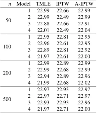
The results in Table 1 confirm the double robustness of the TMLE and A-IPTW, which had been proven analytically in Result 2. The TMLE and A-IPTW are unbiased even for small sample sizes, whereas the IPTW needs larger sample sizes to achieve unbiasedness.
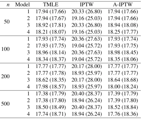
Regarding the variance of the estimators, Table 2 shows that the IPTW estimator is inefficient, and its influence-curve-based variance estimator is very conservative.
The variances of the TMLE and A-IPTW are approximately equal to the efficiency bound if the models for ¯Q0 andg0 are correctly specified, although the same equality is observed if only ¯Q0n is misspecified. This is because, as stated in Result 2, we only need consistent estimation of the weights
Table 1: Expectation of the estimators for different sample sizes and model specifications. True value is 22.95.
n Model TMLE IPTW A-IPTW
50 1 22.99 22.66 22.99 2 22.99 22.49 22.99 3 22.88 22.66 22.91 4 22.01 22.49 22.04 100 1 22.95 22.81 22.95 2 22.96 22.61 22.95 3 22.89 22.81 22.92 4 21.97 22.61 22.00 200 1 22.99 22.89 22.99 2 22.99 22.68 22.99 3 22.94 22.89 22.96 4 21.99 22.68 22.02 500 1 22.97 22.93 22.97 2 22.97 22.71 22.97 3 22.93 22.93 22.96 4 21.97 22.71 22.00
the variance of these estimators is considerably affected by misspecification of the model for ¯Q0(models 3 and 4), even ifg0nis correctly specified. Influence-curve-based estimators of the variance seem to do a good job for these two estimators.
Since all estimators considered are asymptotically linear, 95% normal-based confidence intervals can be computed. Their coverage probabilities are presented in Table (3). The conservativeness of the IPTW can also be appreciated here. The consistent TMLE and A-IPTW based confidence intervals have perfect asymptotic coverage probability. In this simulation we do not observe significant differences between the TMLE and the A-IPTW.
6
Application
With the objective of illustrating the procedure described in the previous sections, we revisit the problem analyzed by Bembom and van der Laan (2007) of assessing the extent to which physical activity in the elderly is associated with reductions in cardiovascular morbidity and mortality, and improvement in, or prevention of metabolic abnormalities. Tager et al. (1998) followed a group of people over 55 years of age living around Sonoma, CA, over a time period of about ten years as part of a longitudinal study of physical activity and fitness (Study of Physical Performance and Age Related Changes in Sonomans -SPPARCS). The goal in analyzing the data that were collected as part of this study is to examine the effect of baseline vigorous LTPA (Leisure Time Physical Activity) on subsequent five-year all-cause mortality. In this paper, we use the same measure of LTPA used by Bembom and van der Laan (2007), which is a continuous score based on the number of hours that the participants were engaged in vigorous
Table 2: Standard error of the estimator (times√n). Expectation of the influence curve based estimator of the variance (times√n) in parentheses. Efficiency bound is 17.81
n Model TMLE IPTW A-IPTW
50 1 17.94 (17.66) 20.33 (26.80) 17.94 (17.66) 2 17.94 (17.67) 19.16 (25.03) 17.94 (17.66) 3 18.92 (17.81) 20.33 (26.80) 18.94 (18.08) 4 18.21 (18.07) 19.16 (25.03) 18.25 (17.77) 100 1 17.93 (17.74) 20.36 (27.63) 17.93 (17.74) 2 17.93 (17.75) 19.04 (25.72) 17.93 (17.75) 3 18.96 (18.14) 20.36 (27.63) 18.98 (18.45) 4 18.34 (18.37) 19.04 (25.72) 18.35 (18.06) 200 1 17.77 (17.77) 20.17 (28.00) 17.77 (17.77) 2 17.77 (17.78) 18.93 (25.97) 17.77 (17.77) 3 18.62 (18.35) 20.17 (28.00) 18.64 (18.68) 4 17.98 (18.57) 18.93 (25.97) 18.00 (18.24) 500 1 17.38 (17.79) 20.40 (28.37) 17.39 (17.79) 2 17.38 (17.80) 18.94 (26.24) 17.39 (17.80) 3 18.50 (18.49) 20.40 (28.37) 18.52 (18.84) 4 17.74 (18.71) 18.94 (26.24) 17.76 (18.36)
physical activities such as jogging, swimming, bicycling on hills, or racquetball in the last seven days, and the standard intensity values in metabolic equivalents (MET: Metabolic Equivalent of Task) of such activities, where one MET is approximately equal to the oxygen consumption required for sitting quietly. The primary confounding factors that we adjust for are described in Table 4. Age and gender are natural confounders, and the rest of the variables intend to account for the subject’s underlying level of general health. Of the 2092 subjects enrolled in the SPPARCS study, 40 were missing information in at least on of this variables; our analysis is based on the remaining 2052 subjects.
In the sequel of this section, the vector containing the confounders will be denoted by W, the continuous MET score byA, and the indicator of five-year all-cause mortality byY. In this paper, we are interested in estimating the effect of a policy that will produce an increase of 12 METs (corresponding, for instance, to bicycling during three hours at less than 10mph per week) in the average of the conditional distribution physical activity, given the covariates. Note that our intervention could also be defined by using different values of MET in each strata defined by the covariatesW.
Initial estimators of the conditional density g0(A|W) and the conditional expectation ¯Q0(A,W)
are presented below.
6.1
Initial estimator of
g
0For the estimation of the density g0(A|W), we consider the estimator presented in D´ıaz and van der
Laan (2011). We now provide a summary of the rationale behind this estimator. Consider k+1 values
Table 3: .
n Model TMLE IPTW A-IPTW
50 1 0.93 0.97 0.93 2 0.93 0.96 0.93 3 0.92 0.97 0.92 4 0.90 0.96 0.89 100 1 0.94 0.98 0.94 2 0.94 0.98 0.94 3 0.93 0.98 0.94 4 0.89 0.98 0.89 200 1 0.95 0.98 0.95 2 0.95 0.97 0.95 3 0.94 0.98 0.95 4 0.87 0.97 0.87 500 1 0.95 0.99 0.95 2 0.95 0.98 0.95 3 0.94 0.99 0.95 4 0.78 0.98 0.78
histogram-like candidate estimators of the conditional densityg0(A|W)
gn,α(A=a|W) =
Prn{A∈[αm−1,αm)|W}
αm−αm−1
, forαm−1≤a<αm−1,
where the choice of the location of α values and the number of bins index the candidates in the class,
and the probabilities in the numerator are estimated through super learner. The final estimator of the den-sity consists of a convex combination of these estimators found through minimization of cross-validated empirical risks. One of the most important properties of this method is that its solution converges to the oracle estimator (i.e., the candidate in the library that minimizes the loss function with respect to the true probability distribution). For further reference and properties of this estimator in the context of estimation of causal effects, the reader is referred to the original paper.
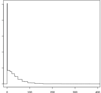
As an example, Figure 1 shows an estimated density gn(A|W) for a particular profileW. As pointed out in D´ıaz and van der Laan (2011), we note that this methodology allows the detection of high density areas in the exposure mechanism, like the one detected at zero in Figure 1. This spike appears because this is a “zero-inflated” exposure, in which a large proportion of the population do not practice any amount of physical activity.
6.2
Initial estimator of
Q
¯
0For the initial estimator of ¯Q0 we used the super learner (van der Laan et al., 2007). Super learner is a machine learning technique that uses cross-validation to choose a convex combination of estimators in a
Table 4: Confounders.
Variable Description Gender Female
Male
Age Age in years
Health
Self-rated health status: Excellent
Fair Poor
NRB Score of self-reported physical functioning rescaled between 0 and 1
Card Previous occurrence of any of the following cardiac events: Angina, myocar-dial infarction, congestive heart failure, coronary by-pass surgery, and coro-nary angioplasty
Chron Presence of any of the following chronic health conditions: stroke, cancer, liver disease, kidney disease, Parkinson’s disease, and diabetes mellitus
Smoking
Never smoked Current smoker Ex-smoker
Decline Activity decline compared to 5 or 10 years earlier
library of candidate estimators. This estimator was also proven to perform asymptotically as well as the oracle selector.
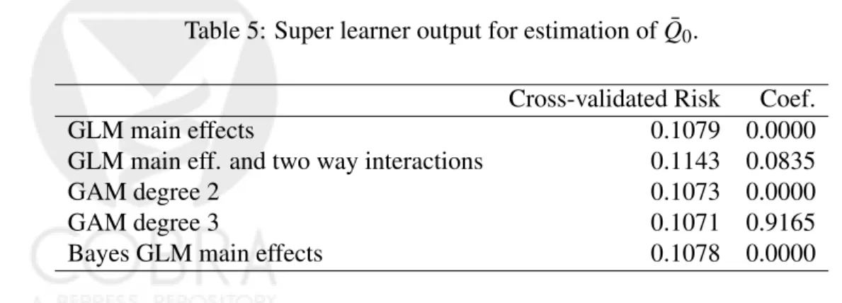
Table 5 shows the candidates used, their cross-validated risks and the weight that the super learner assigns to each of them. It is worth to note that in order to get a consistent estimator of ¯Q0 (sufficient condition for the TMLE ofψ0to be asymptotically unbiased), the library of candidate estimators should
be as large as possible. Since this is an illustrating example, we allow ourselves to use this small library.
Table 5: Super learner output for estimation of ¯Q0.
Cross-validated Risk Coef. GLM main effects 0.1079 0.0000 GLM main eff. and two way interactions 0.1143 0.0835
GAM degree 2 0.1073 0.0000
GAM degree 3 0.1071 0.9165
0 100 200 300 400 0.00 0.02 0.04 0.06 0.08 0.10 A gn
Figure 1: Estimated conditional density of A given the profile age = 73, gender = male, health = fair, nrb = 1, card = yes, smoke = never smoked, decline = yes, and chron = yes.
6.3
Estimators of
ψ
0Table 6 shows the three estimates ofψ0with their standard errors, as described in Section 4.
As an example, the TML estimated value of ψn,3=0.16 indicates that if a policy that increases
the average leisure time physical activity by the equivalent of 12 METs is implemented, the estimated risk of death in the intervened will be 16%.
If the objective is to perform a comparison with the current risk of death, we can define a popula-tion intervenpopula-tion parameterψ01as
ψ01=ψ0−EP0(Y).
This is a parameter that compares the expected risk of death in the intervened population with the current risk of death, and therefore describes the gain obtained by carrying out the intervention of interest. For a given estimatorψnofψ0, an asymptotically linear estimator ofψ01is given byψn1=ψn−Y¯. Its influence
curve can be computed as
D1(P)(O) =D(P)(O)− {Y−EP(Y)},
and its variance is estimated through the sample variance ofD1(P)(O). HereD(P)(O)is the influence curve of each of the estimators defined in Section 4. The estimates of ψ01 and their standard errors are
presented in table 6. Confidence intervals and p-values for hypothesis testing can be computed based on the normal approximations for asymptotically linear estimator described in Section 4 and Appendix A. In light of the results from the simulation section and the theoretical properties of the estimators, we rely on the TMLE and A-IPTW to measure the effect of the intervention of interest. The estimated value of
Table 6: Estimates ofψ0.
TMLE A-IPTW IPTW
ψ0 0.1600(0.0104) 0.1599(0.0105) 0.1454(0.0135)
ψ01 −0.0179(0.0071) −0.0179(0.0071) −0.0324(0.0117)
(corresponding, for instance, to bicycling during three hours per week at less than 10mph) is put in place, the risk of all-cause mortality in the elderly would be reduced by 1.79%. These results are consistent with the findings of Bembom and van der Laan (2007).
7
Discussion
In this paper we define a new parameter for the causal effect of a population intervention that, opposed to most of the parameters presented in the literature, accounts for the fact that in most cases, even after the implementation of the intervention, the exposure continues to be a random variable. We argue that this parameter makes more intuitive sense when the objective is to assess the causal effect of policies intending to modify an exposure variable that cannot be directly intervened upon. For example, as argued in Bembom and van der Laan (2007), it makes little sense to talk about the effect of a static intervention in which every subject in a population of elderly people is required to increase their levels of physical activity to the maximum. It is well known that such intervention will never be possible due to health status and physical functioning constraints, and therefore the causal effect of of such intervention will over estimated the effect of any realistic intervention.
An alternative to overcome this issue, which deals with defining realistic individualized treatment and intention to treat rules is presented in van der Laan and Petersen (2007), and is used in Bembom and van der Laan (2007) to analyze the physical activity data used in Section 6. The choice between that alternative and the one presented in this paper depends on the type of policy for which the effect needs to be estimated. For example, assume that the exposure under study is air pollutants. In that case, we can define individualized pollution regimes for each type of factory, and design a policy intervention that enforces them by law. Under that situation, the effect of individualized deterministic treatment regimes might be more appealing as a way of measuring the effect that such intervention will have in a given outcome. However in examples like the one presented in Section 6, since no deterministic intervention is possible in practice, the causal effect of any population intervention might be better reflected by a causal parameter that takes into account the randomness of the intervention. Three estimators of the parameter were proposed, two of which are double robust to misspecification of the models for the treatment mech-anismg0and the conditional expectation ¯Q0, even when the parameter depends on these two quantities. This double robustness property is proven analytically, and corroborated in a simulation study.
Acknowledgements
We would like to thank Dr. Ira Tager from the Division of Epidemiology at the UC Berkeley School of Public Health for kindly making available the dataset that was used in our data analysis, as well as Tad
Haight and Oliver Bembom for their support in providing information about the dataset.
Appendices
A
Review of Efficiency Estimation in Semiparametric Models
The objective of this section is to provide an intuitive explanation of certain elements of efficient estima-tion in semiparametric models. We do not pretend to give a comprehensive or rigorous review, instead we intend to provide the non trained reader with the basic intuition for understanding why the methods described in the paper work. Careful and detailed definitions of the concepts described here, and rigorous proofs of most of the claims can be found in Bickel et al. (1997) and van der Vaart (1998).
A.1
Asymptotically Linear Estimators
Let X ∼P0∈M, where M is a statistical (semi or non parametric) model, and let Ψ:M 7→R be a
parameter defined as a mapping that takes elements in the model and maps them into the reals (e.g., the meanΨ(P) =RxdP(x)). An estimatorψn ofψ0=Ψ(P0)is called asymptotically linear if there exist a
functionIC:X ×M 7→Rsuch thatIC(·,P0)∈L2(P0),RIC(x,P0)dP0(x) =0 (Bickel et al., 1997), and
ψn−ψ0= 1 n n
∑
i=1 IC(Xi,P0) +oP(n−1/2).The function IC is called the influence function of the estimator, and plays an important role in esti-mation and inference, since it defines the asymptotic variance of the estimator. From the central limit theorem, we conclude that ifψn is asymptotically linear with influence curveIC, then
√ n(ψn−ψ0) d → N{0,P0IC2(·,P0)}.
A.2
Efficiency
Consider a family of parametric submodelsMε ={Pε :ε} ⊂M that coversM and satisfiesPε=0=P0.
A typical choice of family of parametric submodels is{{pε(x) = [1+εs(x)]p0(x):ε}:P0s=0}, where
each parametric submodel is indexed by a functions, which is also its score. The tangent space is defined as the closed linear span of the scores of all parametric submodels. A parameter Ψ is called pathwise
differentiable if there exists a functionν such that for each submodel
dΨ(Pε) dε ε=0 =P0νs.
The functionν is called a gradient of the pathwise derivative. The only gradientDthat is an element of
of any regular asymptotically linear (RAL) efficient estimator, i.e., any RAL estimator whose asymptotic variance equals the efficiency bound (van der Vaart, 1998), which is the semiparametric generalization to the Cramer-Rao lower bound. The efficiency bound is then equal toEP0D2(X).
The efficient influence function has been used by several authors (Bickel et al., 1997, van der Laan and Robins, 2003, Scharfstein, Tsiatis, and Robins, 1997, van der Laan and Rubin, 2006) to con-struct RAL efficient estimators. The basic idea to optimally estimate the parameter of interest is to find estimators that solve the efficient influence curve equation. The properties of estimators that solve a system of equations have been extensively studied in the literature and are provided by the theory of M-estimators. Important references in M-estimation include Bickel et al. (1997), van der Laan and Robins (2003), Tsiatis (2006) and Rose and van der Laan (2011).
A.3
Proofs
Proof. Result 1. First of all, notice that the nonparametric estimator ofψ0is given by
ˆ Ψ(Pn) =
∑
y∈Y a∑
∈Aw∑
∈W yPn(y|a,w)Pn(a−δ(w)|w)Pn(w) =∑
y∈Y a∑
∈Aw∑
∈W yPnfy,a,w Pnfa,w Pnfa−δ(w),w, (9)wherePn= 1n∑ni=1δoi is the empirical measure, fy,a,w=I(Y =y,A=a,W =w), fa,w=I(A=a,W =w)
, fa−δ(w),w=I(A=a−δ(w),W =w), andI(·)denotes the indicator function. HereP f denotesR f dP.
Recall that the efficient influence curve in a non-parametric model corresponds with the influence curve of the non-parametric estimator. This is true because the influence curve of any regular estimator is also a gradient, and a non-parametric model has only one gradient. Rose and van der Laan (2011) show that if ˆΨ(Pn)is a substitution estimator such thatψ0=Ψˆ(P0), and ˆΨ(Pn)can be written as ˆΨ∗(Pnf : f ∈
F)for some class of functionsF and some mappingΨ∗, the influence curve of ˆΨ(Pn)is equal to
IC(P0)(O) =
∑
f∈FdΨˆ∗(P0)
dP0f {f(O)−P0f}.
Applying this result to (9) withF ={fy,a,w,fa,w,fa−δ(w),w}gives the desired result.
Proof. Result 2. Conditioning first on(A,W)and then onW we get
EP0D(O|ψ0,Q¯,g) =EP0 "
∑
a∈A
g0(a|W)
g(a|W)g(a−δ(W)|W){Q¯0(a,W)−Q(a¯ ,W)} # +EP0 "
∑
a∈A g0(a−δ(W)|W)Q(a¯ ,W) # −EP0 "∑
a∈A g0(a−δ(W)|W)Q¯0(a,W) # ,B
R function
tmle.shift()
B.1
Arguments
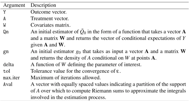
Argument Description Y Outcome vector. A Treatment vector. W Covariates matrix.Qn An initial estimator of ¯Q0in the form of a function that takes a vectorA
and a matrixWand returns the vector of conditional expectations ofY
givenAandW.
gn An initial estimator g0 that takes as input a vector A and a matrixW
and returns the density ofAconditional onW at pointsA.
delta A function ofW defining the parameter of interest.
tol Tolerance value for the convergence ofε.
max.iter Maximum of iterations allowed.
Aval A vector with equally spaced values indicating a partition of the support ofAover which to compute Riemann sums to approximate the integrals involved in the estimation process.
Table 7: Arguments of the R functiontmle.shift
B.2
Code
tmle.shift <- function(Y, A, W, Qn, gn, delta, tol = 1e-5, iter.max = 5, Aval){ # interval partition length
h.int <- Aval[3]-Aval[2]
# this function takes as input initial estimator of Q and g and returns # their updated value
f.iter <- function(Qn, gn, gn0d = NULL, prev.sum = 0, first = FALSE){ # numerical integrals and equation (7)
Qnd <- t(sapply(1:nrow(W), function(i)Qn(Aval + delta, W[i,]))) gnd <- t(sapply(1:nrow(W), function(i)gn(Aval, W[i,])))
gnd <- gnd/rowSums(gnd) if(first) gn0d <- gnd
EQnd <- rowSums(Qnd*gnd)*h.int
D2 <- Qnd - EQnd
QnAW <- Qn(A, W)
H1 <- gn(A - delta, W)/gn(A, W)
# equation (8)
est.equation <- function(eps){
sum((Y (QnAW + eps*H1)) * H1 + (Qn(A + delta, W) EQnd)
-rowSums(D2*exp(eps*D2 + prev.sum)*gn0d)/rowSums(exp(eps*D2 + prev.sum)*gn0d)) }
eps <- uniroot(est.equation, c(-1, 1))$root
gn.new <- function(a, w)exp(eps*Qn(a + delta, w)) * gn(a, w)
Qn.new <- function(a, w)Qn(a, w) + eps * gn(a - delta, w)/gn(a, w)
prev.sum <- prev.sum + eps*D2
return(list(Qn = Qn.new, gn = gn.new, prev.sum = prev.sum, eps = eps, gn0d = gn0d)) }
ini.out <- f.iter(Qn, gn, first = TRUE)
gn0d <- ini.out$gn0d
iter = 0
# iterative procedure
while(abs(ini.out$eps) > tol & iter <= iter.max){ iter = iter + 1
new.out <- f.iter(ini.out$Qn, ini.out$gn, gn0d, ini.out$prev.sum) ini.out <- new.out
}
Qnd <- t(sapply(1:nrow(W), function(i)ini.out$Qn(Aval + delta, W[i,]))) gnd <- t(sapply(1:nrow(W), function(i)ini.out$gn(Aval, W[i,])))
gnd <- gnd/rowSums(gnd) # plug in tmle
psi.hat <- mean(rowSums(Qnd*gnd)*h.int) # influence curve of tmle
IC <- (Y - ini.out$Qn(A, W))*ini.out$gn(A - delta, W)/ini.out$gn(A, W) +
ini.out$Qn(A + delta, W) - psi.hat var.hat <- var(IC)/length(Y)
return(c(psi.hat = psi.hat, var.hat = var.hat, IC = IC)) }
B.3
Example
Here is an example of how to use the previous function based on the data generating mechanism presented in the simulation
n <- 100
W <- data.frame(W1 = runif(n), W2 = rbinom(n, 1, 0.7))
A <- rpois(n, lambda = exp(3 + .3*log(W$W1) - .2*exp(W$W1)*W$W2))
Y < rbinom(n, 1, plogis(1 + .05*A .02*A*W$W2 + .2*A*tan(W$W1^2)
-.02*W$W1*W$W2 + 0.1*A*W$W1*W$W2))
fitA.0 <- glm(A ~ I(log(W1)) + I(exp(W1)):W2, family = poisson, data = data.frame(A, W)) fitY.0 <- glm(Y ~ A + A:W2 + A:I(tan(W1^2)) + W1:W2 + A:W1:W2, family =
binomial, data = data.frame(A, W))
gn.0 <- function(A = A, W = W)dpois(A, lambda = predict(fitA.0, newdata = W,
type = "response"))
Qn.0 <- function(A = A, W = W)predict(fitY.0, newdata = data.frame(A, W, row.names = NULL), type = "response")
tmle00 <- tmle.shift(Y, A, W, Qn.0, gn.0, delta=2, tol = 1e-4, iter.max = 5, Aval = seq(1, 60, 1))
References
O. Bembom and M.J. van der Laan. A practical illustration of the importance of realistic individualized treatment rules in causal inference. Electronic Journal of Statistics, 2007.
P.J. Bickel, C.A.J. Klaassen, Y. Ritov, and J. Wellner. Efficient and Adaptive Estimation for Semipara-metric Models. Springer-Verlag, 1997.
Lauren E Cain, James M Robins, Emilie Lanoy, Roger Logan, Dominique Costagliola, and Miguel A. Hern´an. When to start treatment? a systematic approach to the comparison of dynamic regimes using observational data. The International Journal of Biostatistics, 6, 2010. URL
http://www.bepress.com/ijb/vol6/iss2/18.
Iv´an D´ıaz and Mark J. van der Laan. Super learner based conditional density estimation with application to marginal structural models. 2011. URLhttp://www.bepress.com/ucbbiostat/paper282. F. Eberhardt and R. Scheines. Interventions and causal inference. Department of Philosophy. Paper 415,
2006. URLhttp://repository.cmu.edu/philosophy/415.
A.E. Hubbard and M.J. van der Laan. Population intervention models in causal inference. Technical report 191, Division of Biostatistics, University of California, Berkeley, 2005.
Kevin. Korb, Lucas. Hope, Ann. Nicholson, and Karl. Axnick. Varieties of causal intervention. In Chengqi Zhang, Hans W. Guesgen, and Wai-Kiang Yeap, editors,PRICAI 2004: Trends in Artificial Intelligence, volume 3157 of Lecture Notes in Computer Science, pages 322–331. Springer Berlin / Heidelberg, 2004.
Romain Neugebauer and Mark van der Laan. Nonparametric causal effects based on marginal structural models. Journal of Statistical Planning and Inference, 137(2): 419 – 434, 2007. ISSN 0378-3758. doi: DOI: 10.1016/j.jspi.2005.12.008. URL
http://www.sciencedirect.com/science/article/pii/S0378375806000334.
Maya L Petersen, Kristin E. Porter, Susan. Gruber, Yue. Wang, and Mark J. van der Laan. Diagnosing and responding to violations in the positiv-ity assumption. Stat Methods Med Res, 2010. ISSN 1477-0334. URL
http://www.biomedsearch.com/nih/Diagnosing-responding-to-violations-in/21030422.html. S. Rose and M.J. van der Laan.Targeted Learning: Causal Inference for Observational and Experimental
Data. Springer, New York, 2011.
D.O. Scharfstein, A.A. Tsiatis, and J.M. Robins. Semiparametric efficiency and its implications on the design and analysis of group-sequential studies. Journal of the American Statistical Association, 92 (440):1342–1350, 1997.
Ori M Stitelman, Alan E Hubbard, and Nicholas P. Jewell. The impact of coarsening the explanatory variable of interest in making causal inferences: Implicit assumptions behind dichotomizing variables. 2010. URLhttp://www.bepress.com/ucbbiostat/paper264.
I.B. Tager, M. Hollenberg, and W. Satariano. Self-reported leisure-time physical activity and measures of cardiorespiratory fitness in an elderly population. 1998.
Sarah L Taubman, James M Robins, Murray A Mittleman, and Miguel A Hern´an. Interven-ing on risk factors for coronary heart disease: an application of the parametric g-formula. In-ternational Journal of Epidemiology, 38(6):1599–1611, 2009. doi: 10.1093/ije/dyp192. URL
http://ije.oxfordjournals.org/content/38/6/1599.abstract.
A.A. Tsiatis.Semiparametric theory and missing data. Springer series in statistics. Springer, 2006. ISBN 9780387324487. URLhttp://books.google.com/books?id=xqZFi2EMB40C.
and a general cross-validated adaptive epsilon-net estimator: Finite sample oracle inequalities and examples. Technical report, Division of Biostatistics, University of California, Berkeley, November 2003.
M.J. van der Laan and M.L. Petersen. Causal effect models for realistic individualized treatment and intention to treat rules. International Journal of Biostatistics, 3(1), 2007.
M.J. van der Laan and J.M. Robins. Unified methods for censored longitudinal data and causality. Springer, New York, 2003.
M.J. van der Laan and D. Rubin. Targeted maximum likelihood learning. The International Journal of Biostatistics, 2(1), 2006.
M.J. van der Laan, S. Dudoit, and S. Keles. Asymptotic optimality of likelihood-based cross-validation.
Statistical Applications in Genetics and Molecular Biology, 3, 2004.
M.J. van der Laan, E. Polley, and A. Hubbard. Super learner. Statistical Applications in Genetics and Molecular Biology, 6(25), 2007. ISSN 1.