METHODS FOR HIGH DIMENSIONAL MATRIX
COMPUTATION AND DIAGNOSTICS OF
DISTRIBUTED SYSTEM
A Dissertation
Presented to the Faculty of the Graduate School of Cornell University
in Partial Fulfillment of the Requirements for the Degree of Doctor of Philosophy
by Wei Chen May 2014
c
2014 Wei Chen ALL RIGHTS RESERVED
METHODS FOR HIGH DIMENSIONAL MATRIX COMPUTATION AND DIAGNOSTICS OF DISTRIBUTED SYSTEM
Wei Chen, Ph.D. Cornell University 2014
Big data provides opportunities, but also brings new challenges to modern scientific computing. In this thesis, we conduct sparse principal component analysis (SPCA) on high dimensional matrices. We propose a modified curvilinear algorithm to solve eigenvalue optimization with orthogonal constraints, and combine it with an augmented Lagrangian method to improve its computational efficiency. We compare our algorithm against standard PCA on the recovery of low-rank tensors and a mean-reverted statistical arbitrage strategy. The explosion of big data has also influenced the development on distributed computing systems. For debugging purposes, we are interested in predicting server run-time based on system data early in the process. We study discriminative models in functional data analysis, and introduce generative models that capture server regime-change behaviors. We also design computational methods, including a blocked Gibbs sampler, to improve the accuracy and efficiency of model estimation.
BIOGRAPHICAL SKETCH
Wei Chen was born in Fuzhou, China on December 28, 1984. At the age of fifteen, he entered the talented class of Fuzhou No.3 Middle School. After high school, he moved to Hangzhou to pursue advanced studies at Chu Konchen Honors College of Zhejiang University, where he obtained his Bachelor’s degree with distinction in Mathematics. Upon his graduation from Zhejiang University, Wei decided to continue his education, and joined the Department of Applied Mathematics and Statistics of Johns Hopkins Uni-versity, where he obtained his Master’s degree with distinction in Applied Mathematics. After his graduation, Wei joined the School of Operations Research and Information Engineering at Cornell University as a Ph.D. student. Under the guidance of his advi-sor Martin Wells, he completed his dissertation in the field of Applied Statistics, with a focus on algorithms about sparse principal component analysis, functional data analysis and probabilistic graphical model. During his PhD study, Wei applied his knowledge and skills to various practical problems in the industry, and traveled around the world to collaborate with brilliant professionals from different countries. He interned at Mi-crosoft Research (Mountain View), Nomura Securities (Tokyo), and Goldman Sachs (London) to work on challenging quantitative problems.
Upon graduation from Cornell University with his Ph.D., Wei is excited to pursue his dream in the financial industry, where he has the opportunity to leverage his math, statistics and programming skills.
To my parents:
Maoxin Chen and Yanyan Xu To my wife:
ACKNOWLEDGEMENTS
This thesis could not have been completed without the help and support from many people around me.
First and foremost, I would like to express my deepest gratitude to my advisor, Prof. Martin Wells, for his patient guidance and consistent support throughout my five-year Ph.D. study. He led me to a fascinating realm where statistical modeling and big data applications meet each other. He gave me total freedom to explore my research interest, and offered innovative ideas and warmhearted help on my research and career develop-ment. It is a great honor and privilege for me to work closely and learn from him.
I am very grateful to the other two members in my committee, Prof. Bruce Turnbull and Prof. Ao Tang for their helpful comments and suggestions on my work. I would like to thank the entire faculty at the School of Operations Research and Information Engineering. Their courses and talks broaden my academic horizon and enrich my knowledge.
I would like to acknowledge my supervisor from Microsoft Research, Moises Gold-szmidt, for his interesting computing system project, which becomes a part of my thesis. I would also like to express my thanks to my previous colleagues, Dahua Lin, Qilong Zhang and Paul Kondratko for their career suggestions. I also want to thank Liyan Jia, Yu Zhe, Chaoxu Tong, Cao Ni, Jiayang Gao, Zhengqiang Tang, Liaoruo Wang, and many other friends and students at Cornell University for making my life at Ithaca memorable.
Finally, I would like to thank my parents, Maoxin Chen and Yanyan Xu, for their endless and unconditional love and support; my wife Jing Xie, who stayed with me over the last five years. Her consistent encouragement and advice helped me to challenge tough questions. Without her, I may have given up my Ph.D. study.
TABLE OF CONTENTS
Biographical Sketch . . . iii
Dedication . . . iv Acknowledgements . . . v Table of Contents . . . vi List of Tables . . . ix List of Figures . . . x 1 Introduction 1 1.1 Matrix Computation Problem . . . 1
1.2 Computation System Problem . . . 7
1.3 Thesis Organization . . . 13
2 Hybrid Principal Component Analysis in High Dimensional Low-Rank Ma-trix 16 2.1 Eigenvalue Problems for high dimensional Low-Rank Matrix . . . 17
2.1.1 Reducing matrix inversion by Sherman-Morrison-Woodbury . . 18
2.1.2 Line Search with Barzilai-Borwein steps . . . 19
2.1.3 Numerical Results in Linear Eigenvalue Problem . . . 20
2.2 Algorithm for Sparse Principal Component Analysis . . . 22
2.2.1 Hybrid Principal Component Analysis (HPCA) . . . 22
2.2.2 Numerical Results of HPCA in Sparce Principal Component Analysis . . . 24
2.3 Application of HPCA in Equity Statistical Arbitrage . . . 27
2.3.1 Problem Formulation . . . 28
2.3.2 Methods for Modeling Market Factors . . . 29
2.3.3 Trading Signals and Arbitrage Strategy . . . 31
2.3.4 Backtesting Results . . . 33
2.4 Conclusion . . . 36
3 Hybrid Principal Component Analysis in Low-Rank Tensor Estimation 38 3.1 Matrix and Tensor . . . 38
3.1.1 Rank and Trace Norm . . . 38
3.1.2 Tensor Representation and Rank . . . 39
3.2 Trace Norm Penalization for Reconstruction of Low-Rank Tensor . . . 40
3.2.1 Single Unfolding Penalization . . . 40
3.2.2 Multiple Unfolding Penalization . . . 41
3.2.3 Mixture Unfolding Penalization . . . 42
3.3 Optimization for Trace Norm Penalization . . . 42
3.3.1 ADMM . . . 43
3.3.2 HPCA in ADMM . . . 44
3.4 Numerical Results for Reconstruction of Low-Rank Tensor . . . 45
4 Discriminative Methods for Predicting Process Run Time in Computing
Systems 50
4.1 Estimation Methods . . . 51
4.1.1 Penalized Functional Regression . . . 53
4.1.2 A Simpler FDA Method . . . 55
4.1.3 Generalized Linear Model . . . 56
4.1.4 Functional Quadratic Regression . . . 56
4.1.5 Bayesian Penalized Functional Regression . . . 57
4.2 Application to DryadLINQ . . . 58
4.3 Classification Application to DryadLINQ . . . 60
4.3.1 Results from “Click Bot” . . . 62
4.3.2 Results from other datasets . . . 65
4.4 Prediction of the Run Time on DryadLINQ . . . 67
4.4.1 Results from “Click Bot” . . . 67
4.4.2 Results from other datasets . . . 70
4.5 Conclusion . . . 71
5 Generative Methods for Predicting Process Run Time in Computing Sys-tems 72 5.1 Hidden Markov Regime-Change Autoregression . . . 74
5.2 Hidden Markov Autoregression . . . 79
5.3 Hidden Semi-Markov Regime-Change Autoregression . . . 80
5.3.1 Small Step: Adjust Starting Time for Segments . . . 83
5.3.2 Large Step: Merge and Split Segments . . . 84
5.4 Blocked Gibbs Sampling . . . 88
5.5 Numerical Results from DryadLINQ . . . 91
6 Conclusions 97 A Appendix of Chapter 4 99 A.1 Discriminative Methods: Binary Classification in “Click Bot” . . . 99
B Appendix of Chapter 5 102 B.1 Gibbs Sampling for HMRCA . . . 102
B.1.1 Transition MatrixQ . . . 102 B.1.2 Regime IndicatorZn,t . . . 103 B.1.3 Regime Meanµk,t . . . 104 B.1.4 Regime Varianceσk2 . . . 107 B.1.5 Regression Coefficienta . . . 108 B.1.6 Regression Varianceσε2 . . . 109
B.2 Blocked Gibbs Sampling for HMRCA . . . 111
B.2.1 Blocked Gibbs Sampling forµk,t . . . 111
B.2.2 Blocked Gibbs Sampling forZn,t . . . 114
B.3.1 Regime IndicatorZn . . . 116
B.3.2 Regime Meanµk,t . . . 117
B.3.3 Regime Varianceσk2 . . . 120
B.4 Blocked Gibbs Sampling for HMA . . . 121
B.4.1 Blocked Gibbs Sampling forµk,t . . . 121
B.5 Metropolis-within-Gibbs for HSMRCA . . . 124
B.5.1 Transition Matrix Q . . . 124
B.5.2 Segment IndicatorZn∗,l . . . 124
B.5.3 Sojourn Time Meanλ . . . 125
C Appendix of Chapter 6 126 C.1 Generative Methods: Binary Classification in “Click Bot” . . . 126
LIST OF TABLES
2.1 Comparision of eigenvalue calculation on random matrices with p = 6 . 20 2.2 Comparision of eigenvalue calculation on random matrices with n =
10000 . . . 21
2.3 Comparision of eigenvalue calculation on real sparse matrices from Sparse Matrix Collection - CISE.UFL . . . 21
2.4 Comparision of SPCA methods on randomly generated full-rank ma-trices with p=6 . . . 26
2.5 Comparision of SPCA methods on randomly generated low-rank ma-trices with p=6 . . . 27
2.6 Comparision of factoring approaches on a $100 portfolio fromS&P500 36 3.1 Tensors in numerical simulations . . . 46
4.1 Discriminative Methods: Binary Classification Results from “Click Bot” Dataset . . . 63
4.2 Binary Classification Results from Three Datasets . . . 66
4.3 Continuous Prediction Results from “Click Bot” Dataset . . . 70
4.4 Continuous Prediction Results from Three Datasets . . . 70
5.1 Effective sample sizes for selected variables in HMRCA . . . 90
5.2 Generative Methods: Binary Classification Results from “Click Bot” Dataset . . . 95
LIST OF FIGURES
1.1 Variance in running time for a given stage in a program for detecting ClickBots. Notice that a few vertices (horizontal lines) are responsible
for most of the waiting time. . . 9
2.1 Value of a $100 portfolio fromS&P500 . . . 34
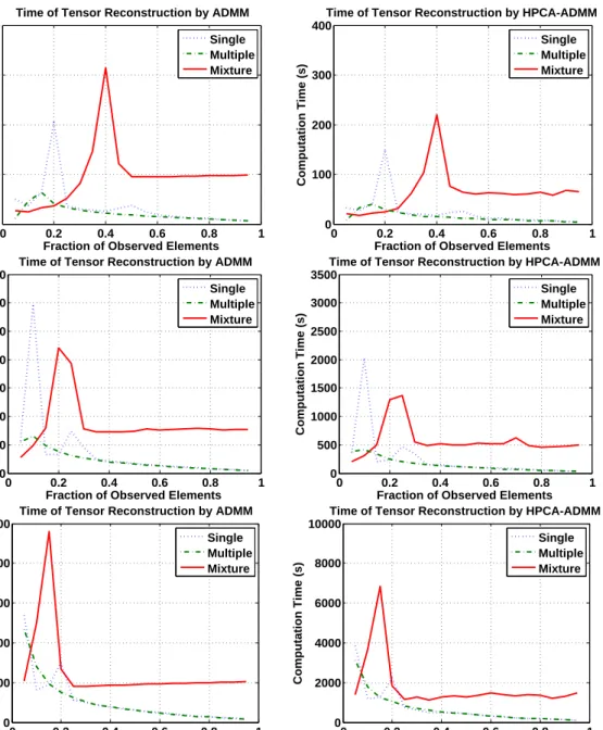
3.1 Computation of ADMM and HPCA-ADMM in Tensor Reconstruc-tion with rank(3,4,5)and dimensions: (1) (100,100,40) (above), (2) (500,500,200)(middle),(1000,1000,400). . . 48
3.2 Computation of ADMM and HPCA-ADMM in Tensor Reconstruc-tion with rank(7,8,9)and dimensions: (1) (100,100,40) (above), (2) (500,500,200)(middle),(1000,1000,400). . . 49
4.1 CPU utilization during the “Click Bot” job, for servers having run time below the tolerance level (left), and above the tolerance level (right). . . 59
4.2 Memory utilization during the “Click Bot” job, for servers having run time below the tolerance level (left), and above the tolerance level (right). 59 4.3 Discriminative methods: ROC Curve (left) and Cost Curve (right) from “Click Bot” Data in multi-metrics . . . 64
4.4 Estimated beta functions from “Click Bot” Data in the processor met-ric (left) and the memory metmet-ric (right) for the three cross-validation training sets . . . 65
4.5 (1) CPU utilization during the “Bot Tracker” job, for servers hav-ing run time below the tolerance level (left), and above the tolerance level (right). (2) Examples of the estimated beta functions from “Bot Tracker” Data (bottom) for the three cross-validation training sets . . . 68
4.6 Root Mean Squared Error (left) and Mean Absolute Error (right) in “Click Bot” Data, and the estimate beta function in the memory metric in “Click Bot” Data (bottom) . . . 69
5.1 The graphical model of HMRCA . . . 74
5.2 The graphical model of HMA . . . 79
5.3 The graphical model for HSMRCA . . . 82
5.4 The small step ofτn,l . . . 83
5.5 The large step ofτn,l . . . 84
5.6 Means of Regimes from HMRCA for CPU utilization during the “Click Bot” job, for servers having run time below the tolerance level (left), and above the tolerance level (right). . . 93
5.7 Generative methods: ROC Curve (left) and Cost Curve (right) from “Click Bot” Data in multi-metrics . . . 96
A.1 Discriminative methods: ROC Curve (upper left) and Cost Curve (up-per right) from “Click Bot” Data in processor metric, ROC Curve (lower left) and Cost Curve (lower right) from “Click Bot” Data in
memory metric . . . 99
A.2 Discriminative methods: ROC Curve (upper left) and Cost Curve (up-per right) from “Click Bot” Data in disk metric, ROC Curve (lower left) and Cost Curve (lower right) from “Click Bot” Data in network metric 100 A.3 Estimated beta functions from “Click Bot” Data in the disk metric (left) and the network metric (right) for the three cross-validation training sets 101 B.1 The local graphical model for Q . . . 102
B.2 The local graphical model forZn,t . . . 103
B.3 The local graphical model forµk,t . . . 104
B.4 The local graphical model forσk2 . . . 107
B.5 The local graphical model fora . . . 108
B.6 The local graphical model fora . . . 109
B.7 The local graphical model forZn . . . 116
B.8 The local graphical model forµk,t . . . 117
B.9 The local graphical model forσk2 . . . 120
C.1 Generative methods: ROC Curve (upper left) and Cost Curve (upper right) from “Click Bot” Data in processor metric, ROC Curve (lower left) and Cost Curve (lower right) from “Click Bot” Data in memory metric . . . 126 C.2 Generative methods: ROC Curve (upper left) and Cost Curve (upper
right) from “Click Bot” Data in disk metric, ROC Curve (lower left) and Cost Curve (lower right) from “Click Bot” Data in network metric 127
CHAPTER 1 INTRODUCTION
According to McKinsey’s Business Technology Office (MBT), the ability of analyzing so-called “big data” will become a key basis of competition, and a basis for new waves of productivity, growth and innovation. What was the domain of companies like Mi-crosoft, Google, Yahoo, Facebook, and Amazon, namely, crunching through terabytes to petabytes of data for services such as search, social networks, customer preferences, and news portals, up to about 5 years ago, is becoming the focus of more and more companies on all sectors including government. MBT estimates that by 2009 nearly all sectors in the US economy had at least an average of 200 terabytes of stored data (twice the size of Wal-Mart’s data warehouse in 1999) per company with more than 1,000 employees. This data includes business intelligence data, (e.g. consumer baskets and habits, marketing data, etc), and data about the processes in the companies themselves, and data about sentiment on companies products and services gathered from the web and the social networks themselves.
1.1
Matrix Computation Problem
The invention of internet moves us from the traditional text-based communication to the new interactive media, while improvements in data storage technology makes it possi-ble to save enormous amount of data directly or indirectly from users, markets, or even environment (Michael and Miller 2013). Big data can help us explore people’s behavior patterns. For instance, some social network companies and electronic commerce com-panies can analyze customers’ characteristics from their social connections or shopping records, and predict their interests and decision making processes; big data can also
pro-vide us some valuable insights to the hidden disciplines of the markets. For instance, some algorithmic trading companies can trade against some statistical mispriced secu-rities to make profits if they study price relationships between thousands of secusecu-rities in the market; big data can even lead to discovery of prevention or cures for some dis-eases. The Human Genome Project and Human Brain Project are typical bioinformatic efforts researchers have done so far. However, big data brings not only opportunities, but also challenges to modern data analysis, which requires robust and efficient analysis approaches. Fan et al. (2013) pointed out that big data has two important characteris-tics: high dimensionality and large sample size. The challenges raised by these two features include noise accumulation, spurious correlations, homogeneity, heterogeneity, and computational costs. Many traditional methods perform well in low dimensional or moderate sample size, but do not scale to high dimensional or large sample size.
To face the challenges of big data, technology about dimension reduction and vari-able selection has been extensively studied and employed in data analysis. For instance, various regularization and variable selection methods are developed over the last few decades (Fan et al. 2013), including shrinkage via lasso (Tibshirani 1996), signal de-composition via basis pursuit (Chen et al. 1998), nonconcave penalized likelihood (Fan and Li 2001), Dantzig selector (Candes and Tao 2007), minimax concave penalty (Zhang et al. 2010) and etc. We specifically consider principal component analysis (PCA) (Jol-liffe 1986), which is one of the most popular dimension reduction techniques and has been widely used in scientific applications, e.g., image recognition (Hancock et al. 1996), gene expression (Alter et al. 2000), natural language processing (Hastie et al. 2005), and etc. Variations of PCA include functional PCA (Friston et al. 1993), nonlin-ear PCA (Sch¨olkopf et al. 1998), probabilistic PCA (Tipping and Bishop 1999), multino-mial PCA (Buntine 2002), kernel PCA (Scholkopf et al. 1999), generalized PCA (Vidal et al. 2005), sparse PCA (Zou et al. 2006) and etc.
Sparse principal component analysis (SPCA) is one of the most efficient PCA meth-ods under the big data scenario. The main drawback of PCA is the low interpretability of principal components (PCs), especially when we apply PCA to high dimensional data. SPCA fixes this issue by generating principal components with a lot of zero load-ings. There is substantial work on SPCA over the last few decades. The first class of SPCA is the heuristic modification of PCs from the standard PCA, e.g., factors rota-tion (Jolliffe 1995), artificial threshold of eigenvectors (Cadima and Jolliffe 1995); the second class is the optimization formulation of SPCA, e.g., LASSO based PCA (Jolliffe et al. 2003), nonconvex approximation (Zou et al. 2006, Sriperumbudur et al. 2007); the third class is the spectral analysis and singular value decomposition (Moghaddam et al. 2006, 2007, Shen and Huang 2008); and the fourth class is semidefinite programming (SDP) (D’Aspremont et al. 2007, d’Aspremont et al. 2008, Zhang and El Ghaoui 2011). For other theoretical work on SPCA, see Journ´ee et al. (2010), Amini and Wainwright (2008), Yuan and Zhang (2011), Asteris et al. (2011).
Although the above SPCA methods eventually obtain sparse PCs, they do not take the correlation of PCs into account – some methods do not even consider the orthogo-nality of loading vectors. Moreover, these methods over maximize the total explained variance of sparse PCs. Lu and Zhang (2012) pointed out these two issues and proposed their formulation of SPCA:
max X∈Rn×ptr(X T ΣX)−ρ|X| s.t. |XiTΣXj| ≤∆i,j, XTX =I, (1.1)
where∆i,j≥0(i6= j)are tuning parameters for the correlation ofX, andρ>0 is the
pe-nalized parameter of sparsity. This formulation improves upon the other SPCA methods by introducing additional constraints. To solve (1.1), Lu and Zhang (2012) introduced
an augmented Lagrangian algorithm, and proved its convergence under certain assump-tions. They also mentioned the importance of finding an starting point when applying the algorithm to high-dimensional matrices.
In this thesis, we propose an algorithm for finding a feasible starting point. Instead of choosing a starting point randomly (Lu and Zhang 2012), we solve a generalized problem of (1.1)
max X∈Rn×ptr(X
T
ΣX) s.t. XTX =I, (1.2)
which can be classified as a manifold optimization problem, since the feasible set {X :XTX =I} of (1.2) is Stiefel manifold. A variety of algorithms have been pro-posed during the last few decades for manifold optimization, including retraction algo-rithms (Adler et al. 2002, Absil et al. 2007, Baker et al. 2008, Absil et al. 2009), steepest descent gradient (Helmke et al. 1994, Udriste 1994), conjugate gradient (Edelman et al. 1998, Qi et al. 2010) and Newton’s method (Smith 1994, Owren and Welfert 2000, Smith 2013). These algorithms typically preserve the manifold constraints during the iterations.
In recent literature, Wen and Yin (2013) proposed a curvilinear algorithm to solve (1.2). We improve their algorithm in the computational efficiency of the large matrices computation, and incorporate it with the augmented Lagrangian algorithm. We compare the hybrid algorithm against other existing SPCA methods on randomly gen-erated matrices. Our results show that our hybrid algorithm is computationally more efficient than the existing methods.
In terms of application, we apply our algorithm to a mean-reverted statistical arbi-trage strategy (Avellaneda and Lee 2010), and show its performance on trading signals ofS&P500 from 2007 to 2013. Statistical arbitrage is a variety of trading and invest-ment strategies, and has been extensively studied since 1990s (Poterba and Summers
1988, Lehmann 1990, Lo and MacKinlay 1990, Admanti and Pfleiderer 1991, Barclay and Warner 1993, Miller et al. 1994, Chan and Lakonishok 1993, 1995, Bollerslev and Ole Mikkelsen 1996, Davis et al. 1997, Lo 1999, Bookstaber 2000, Lo 2001, Cont et al. 2002, Boss et al. 2004, Andersen et al. 2006, Khandania and Lob 2007, Avellaneda and Lee 2010).
In a generic statistical arbitrage strategy, investors create a market-neutral portfolio with low volatility, by pairing up a large number of stocks to diversify the risk. We particularly consider a mean-reverted strategy. In this strategy, we decompose the stock return into two parts, a systematic part and an idiosyncratic part. We model the system-atic part by regressing it on some other reference returns (called “market factors”), and model the idiosyncratic part by a mean reversion process. Statistical arbitragers believe that if market factors are chosen wisely to diversify the systematic risk, the idiosyncratic return will oscillate around its long-run mean. This provides an opportunity for them to lock their profit by shorting the stock when the idiosyncratic return is above the long-run mean, and longing the stock when the idiosyncratic return is below the long-long-run mean. Avellaneda and Lee (2010) studied two methods for generating market factors, mainly, standard PCA and exchange-traded funds (ETFs), based on trading signals of
S&P500 from 2003 to 2007. Although they are easy to implement, issues remain:
1. Derived portfolios from PCA are difficult to interpret.
2. Trading each constituent of portfolios from PCA takes extra transaction cost. 3. ETFs contain correlated information.
4. ETFs requires prior information about the economy and the market.
In Chapter 2, we use SPCA to generate market factors, and compare its performance against PCA and ETFs. We show that SPCA simplifies the components of derived
portfolios, reduces the transaction costs, and performs uniformly better than PCA and ETFs.
We also apply our hybrid algorithm to low-rank tensor estimation. Tensor, also known as multi-dimensional array, is used to represent relationships between sets of geometric vectors. It has been widely used in physics (Danielson and Danielson 1997, Chaikin and Lubensky 2000, Jeevanjee 2011), psychometrics (Grieve et al. 2007, Kodl et al. 2007), chemometrics (Kolda and Bader 2009, Lim and Comon 2009), signal pro-cessing (De Lathauwer and De Moor 1998, De Lathauwer et al. 2000a, Westin et al. 2002), computer vision (Hartley and Zisserman 2003, Medioni and Kang 2004, Shashua and Hazan 2005, Aja-Fern´andez 2009), neuroscience (Martınez-Montes et al. 2004, Mi-wakeichi et al. 2004, Damoiseaux et al. 2006), and elsewhere. Under the big data sce-nario, decomposition and interpretation of tensors have become more and more impor-tant. Many tensor decomposition methods have been proposed over the last few decades, like INDSCAL (Carroll and Chang 1970), PARAFAC2 (Harshman 1972), DEDI-COM (Harshman 1978), CANDELINC (Carroll et al. 1980), PARATUCK2 (Harshman and Lundy 1996). Among all, CANDECOMP/PARAFAC (Carroll and Chang 1970, Harshman 1970) and Tucker (Tucker 1966, De Lathauwer et al. 2000b) are the most popular ones nowadays. However, these methods use non-convex optimization for esti-mating tensors, which suffers certain convergence issues.
Recently, convex optimization has been introduced to the estimation of two– dimensional tensor (Fazel et al. 2001, Srebro et al. 2004, Evgeniou and Pontil 2007, Tomioka and Aihara 2007), with development of theory on matrix reconstruc-tion (Cand`es and Recht 2009, Recht et al. 2010). The estimareconstruc-tion has also been general-ized to tensors with higher dimensions (De Silva and Lim 2008, Signoretto et al. 2010, Gandy et al. 2011, Liu et al. 2013, Rauhut et al. 2013). Tomioka et al. (2010) proposed
three convex formulations for the low-rank tensor reconstruction, and solved their prob-lems by alternating direction method of multipliers (ADMM) (Gabay and Mercier 1976, Boyd et al. 2011). In Section 2.2, we apply our hybrid algorithm to ADMM, show that the modified algorithm performs roughly 25% faster than ADMM.
Other optimization work about large-scale computing include random sampling in convex programming (Bertsimas and Vempala 2004), mixed integer optimization on least quantile of squares (Bertsimas and Mazumder 2013), mixed integer programming with automated configuration (Hutter et al. 2010), Global mixed-integer quadratic opti-mizer (Misener and Floudas 2013), robust optimization (Bertsimas et al. 2011), interior point method with warm-start point (Colombo et al. 2011), interior point method with
l1-regularized least squares (Kim et al. 2007), and some optimization software for large scientific programming, like CPLEX (Cplex 2007, CPLEX 2009) and Gurobi (Opti-mization 2012) are also developed and widely used in both academia and industry.
1.2
Computation System Problem
The explosion of the availability of data has also influenced a parallel development on the computing infrastructure. This infrastructure consists of software, which takes a linear program, distributes and parallelizes its application into large clusters of ma-chines. These platforms include Google’s Map/Reduce, Yahoo’s Hadoop, and Microsoft Dryad (Isard et al. 2007, Yu et al. 2008). Estimates vary but these platforms are widely used with Yahoo running more than 40,000 nodes of Hadoop with their biggest single cluster now at 4,500 servers. Facebook runs a 1,100 node cluster and a second 300 node cluster. LinkedIn runs many clusters including deployments of 1,200,580, and 120 nodes. What has not been keeping with this rapid development are tools and methods for
debugging the performance of these systems. This thesis starts to address this problem in a statistically sound approach.
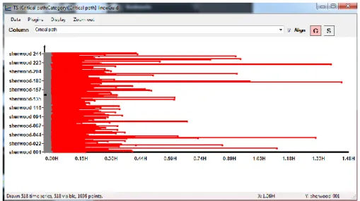
In general, these computing platforms are (loosely) based on the map/reduce model, first reported in the literature (in the context of big data) in Dean and Ghemawat (2008). Very loosely, in this model the computation proceeds in stages where each stage is either amapstage or areducestage. Each stage is composed of a set of nodes performing the same computation in parallel on different partitions of the data. Themapstage executes the same operation (may be a complex piece of code) in all nodes and each node in thereducestage consumes the output of various nodes in the map stage and so on. As all nodes in a particular stage (either map or reduce) perform the same operation, it is expected that their running time should be similar. In practice, this is not always the case. The problem is that a single outlier may destroy the inherent parallelism, as for example the whole reduce stage will not start until the preceding map stage finishes. Thus the running time of the whole program, suddenly depends on a single outlier. Figure 1.1 shows this phenomena on a real computation. This program applies machine learning algorithms to analyze clicking behavior in order to detect clicking-robots. The horizontal axis is time (in fractions of hours) and the vertical axis are physical machines. A horizontal line represents the running time of a machine. Note that a handful of outliers, approximately 15 out of 250 machines, cause total running time of the stage to extend from 30 minutes to one hour and 30 minutes.
There are many possible causes of this misbehavior: (a) it can be that the initial partition of the data is not balanced and some nodes consume more data than others (hence the computation takes longer); (b) It can be that the node is not reading the data from a local disk but over the network, or from a congested disk; (c) it can be that the node is faulty (there is a hardware problem). In any case an early detection of an outlier
Figure 1.1: Variance in running time for a given stage in a program for detecting ClickBots. Notice that a few vertices (horizontal lines) are responsible for most of the waiting time.
is beneficial for various reasons: First, we can use it to estimate the running time of the whole program. Second, we can alert the job manager of the situation so that diagnostics can be executed on the node to determine whether it is faulty. If it is the case that the node is faulty, then a duplicate node can be activated to continue with the job. Note that duplication is not always a beneficial action. For example, if the slowness of the node is due to the fact that it is reading from a physical disk that is congested (because too many other vertices are sharing it) duplicating the node will only exacerbate the problem. It may be possible to execute other more complicated actions such as on the fly reallocation of computational nodes (to balance the load on disks), or change the dependency between the different nodes in the different stages.
In this thesis, we introduce the classification models to predict whether the server processing time will be normal based on server metrics. The modeling is inspired by two different methodologies, discriminative and generative methods. In a discrimina-tive method, a parameter model is introduced to compute the mappings between latent variables and observed variables directly, and the values of parameters are inferred from
the training data; while in a generative method, a joint distribution of both latent and ob-served variables is proposed and estimated. This can be done, for instance, by learning the priors of latent variables and conditional distributions of observed variables sepa-rately, and obtaining the posterior distribution by Bayes theorem.
We provide two different models, one from each method. The first one is functional linear model, a type of functional data analysis approach. It is a distriminative method, since we link the running time of servers and its metrics by logistic functional regression. Functional data analysis (FDA) is an effective approach for analyzing data from curves and surfaces, and has recently received substantial interest in the statistics literature. It has also been applied to scientific and industrial settings extensively. Specifically we use methods for regression with functional predictors and a scalar outcome (Ramsay 2006, Ramsay and Silverman 2002). The predictors in our context are the time series obser-vations of the server metrics, while the outcome is either the real-valued run time or a binary indicator of whether the run time is above a specified tolerance. Instead of treat-ing the time series observations as separate predictors, the FDA approach treats them as noisy, discrete observations of unknown continuous functions. These functions are related to the scalar outcome via a model such as the functional linear model (Cardota et al. 1999).
This FDA approach has several advantages for prediction and interpretation. First, since the time series structure of the predictors is built into the model, the signal and noise in that time series predictor can be distinguished more accurately. Effectively the time series predictors are smoothed over time, so that information from the whole time series is used to remove the noise in each observation. This improves predictive accuracy of the regression model. Second, the FDA model relating the functional predictor to the outcome can be much more interpretable than the output of a simpler regression model.
For instance the functional linear model relates the outcomeW to a predictor function
X(t)via
g(EW) =α+ Z
CX(t)β(t)dt, (1.3)
where g is referred to as the “link” function, α is the intercept, W is a real random
response, EW is the expected value ofW, and X(t), β(t) are square integrable
ran-dom functions defined on some compact set C of R. The coefficient function β(t)is
smoothly estimated, and the sign and magnitude ofβ(t)over time indicates the
relation-ship betweenX(t)andEW.
The method of Goldsmith et al. (2010) is based on the functional linear model. We apply this method, as well as several related approaches, to the problem of predicting server run-time in a commercial computing system (Microsoft’s DryadLINQ (Isard et al. 2007, Yu et al. 2008)). We compare their performance to that of an additive generalized linear model that uses the time series observations as separate predictors. Our results show that the FDA methods have better classification accuracy when predicting the bi-nary indicator of whether the run time exceeds a specified tolerance. A cost analysis shows that this yields up to a 20% lower cost associated with classification errors. For predicting the continuous run time, the method of Goldsmith et al. (2010) has roughly 5% lower errors. We also find that the FDA methods yield far more interpretable re-sults. These results show the value added by using FDA methods in computing system management.
The other model is Hidden Markov/Semi-Markov Regime-Change Autoregression model (HMRCA/HSMRCA), which is based on hidden Markov/semi-Markov model except that it has multiple regimes and allows regime switching for sample series, and the mean of regimes follow autoregression process. This novel model is proposed re-garding that the characteristics of the distributed computing data are not captured
ef-fectively using the linear model approach. The reason is that each server goes through phases of accessing data, doing computation, waiting for sub-task completion by ex-ternal systems, etc., and that the duration of each phase is stochastic. Incorporating regime-change behavior into this new model will allow us to simulate the different phases each server goes through. This novel generative model can capture some be-haviors that some discriminative models cannot, for instance, differences in variability of the time series for different values of the outcomes. Besides that, we also design and implement a blocked Gibbs sampling to draw sample series directly from the posterior distributions of time series parameters in Hidden Markov Regime-Change Autoregres-sion model (HMRCA).
Hidden Markov model (HMM), as one of the most famous generative probabilistic model, is widely used in different research areas, like signal recognition (Juang and Ra-biner 1991, Andrieu and Doucet 1999), computational biology (Leroux and Puterman 1992, Krogh et al. 1994), genomics (Churchill 1992, Liu et al. 1999), image process-ing (Choi et al. 2000), econometrics (Hamilton 1989, 1990, Albert and Chib 1993) and elsewhere. HMM assumes that there is a set of statesS ={1,2, . . . ,S}and the asso-ciated distributions{Fi}for each statei=1,· · ·,S. The time series observations{Xt},
t =1, . . . ,T, depend on their unobserved hidden states{Zt},t =1, . . . ,T, which follow a Markov chain onS with transition matrixQQQ={Qi,j},i,j=1, . . . ,S.
P(Zt|Zt−1) =QZt−1,Zt and P(Xt|Zt) =FZt(Xt). (1.4)
As an extension of HMM, hidden semi-Markov model (HSMM) allows the underlying stochastic process of{Zt},t=1,· · ·,T, to be semi-Markov chain with sojourn time. The main difference between HMM and HSMM is that HMM only allows one observation for each state while each state can generate a sequence of observations in HSMM (Yu 2010, Si et al. 2011).
The regime-switching idea has existed for a long time in econometric commu-nity (Van Norden and Vigfusson 1996, Piger 2009). From time to time, economic data exhibit dramatic changes, associated with short-term events like financial crises, changes in government policies or long-term events like economic recessions. Con-sequences of those changes are described by different regimes. In early literature of econometrics, the underlying model for each regime is the same, such asAR(1), and the regime-switching time follows a Markov chain; while in more complex models, high dependencies among observations are considered, and the coefficients are also subject to changes in regimes (Hamilton 2005, Kim and Nelson 1999). In Chapter 5, we have similar regime-switching properties in HMRCA/HSMRCA. We differ from the above literature in two main aspects: (1) the underlying parameters are also assumed to follow some processes. (2) priors for parameters are chosen carefully to avoid serious problems with hierarchical models.
We compare the HMRCA/HSMRCA against a parsimonious model without change property, Hidden Markov Autoregression (HMA), and find that the regime-change design improves the prediction accuracy by reducing 20% of the classification errors and 30% of the associated costs. We also find that HMRCA/HSMRCA obtain similar accuracy with PFR, and both models are highly recommended in computing system diagnostics.
1.3
Thesis Organization
In this section, we summarize the contents of each chapter.
Chapter 2 considers the problem of SPCA in low-rank matrices. We first discuss a convex optimization problem with orthogonal constraints, and propose a modified
curvi-linear algorithm to solve it. We then develop an hybrid algorithm by incorporating the modified curvilinear algorithm into an augmented Lagrangian algorithm, and show that our hybrid algorithm is computationally better than the original augmented Lagrangian algorithm. We also consider a mean-reverted statistical arbitrage strategy, and apply our hybrid algorithm to generate market factors for the strategy. We backtest the strategy on historical data ofS&P 500, and show that SPCA performs better than PCA and ETFs methods with lower transaction costs and more interpretable portfolios.
Chapter 3 addresses the low-rank tensor estimation. We discuss three convex for-mulation for the reconstruction of low-rank tensor, and the existing algorithm ADMM. We then apply our hybrid algorithm to ADMM to improve its computation efficiency, and show numerically that the new algorithm performs better than ADMM in all three formulations with similar recovery rates and shorter computation time.
Chapter 4 considers the discriminative methods for predicting running time of servers in large-scale computing systems. We first discuss the map/reduce design of the parallel computing systems, and the associated diagnostic problems in practice. We then study the penalized functional regression, and apply our hybrid algorithm to improve it. We compare it against an additive generalized linear model and logistic regression on four datasets from DyradLINQ of Microsoft. We study the performance of three meth-ods in binary classification and continuous prediction. Our results show that penalized functional regression is uniformly better than the other two methods. We suggest it in predicting running time servers in large-scale computing systems.
Chapter 5 studies the generative methods for diagnostics of large-scale computing systems. We propose three data-driven models, HMRCA, HSMRCA and HMM, to classify the servers in computing systems. HMRCA and HSMRCA are designed to capture the regime-switching behavior we observe from data. We also discuss the
es-timation problems of Monte Carlo simulation in these models, and design a blocked Gibbs sampling algorithm to improve the convergence of simulated Markov chain. We apply our models to the datasets from DyradLINQ of Microsoft, and show that the regime-switching property improves the classification accuracy.
CHAPTER 2
HYBRID PRINCIPAL COMPONENT ANALYSIS IN HIGH DIMENSIONAL LOW-RANK MATRIX
Matrix orthogonality constraints have important influence in many scientific re-search areas. In particular, minimization with the orthogonality constraints is widely used in polynomial computation, combinatorial mathematics, eigenvalue calculation, sparse principal component analysis, matrix rank specification, etc. These problems are challenging because the constraints are computationally expensive to preserve during iterations.
One of the interesting problems is the following optimization problem with orthog-onality constraints,
min
X∈Rn×pF(X) s.t. X
TX=I (2.1)
where I is the identity matrix and F(X) is a differentiable function. This problem is difficult because it is challenging to directly solve the nonlinear and nonconvex con-straints. As a result, iterative methods are commonly used instead. An curvilinear search algorithm (Algorithm 1, see below) was previously proposed in Wen and Yin (2013) to solve (2.1), and was proved to be efficient and robust in various test cases. However, the application of Algorithm 1 in high dimensional low-rank matrices were not carefully discussed in Wen and Yin (2013). In Section 2.1, we propose a modified curvilinear al-gorithm to solve the linear eigenvalue problem for high dimensional low-rank matrices.
Principal component analysis (PCA) is a classical method for data analysis and di-mension reduction. However, each principal component is a linear combination of all the original attributes, so it is difficult to interpret the result. Sparse principal component analysis (SPCA) extends standard PCA, and produces more zero loadings in modified
principal components. In Section 2.2, we apply the modified curvilinear algorithm in Section 2.1 to an augmented Lagrangian method (Lu and Zhang 2012).
Algorithm 1:A gradient descent curvilinear algorithm (2.1)
1 Given an initial pointX0withX0TX0=I; 2 Setk=0,ε≥0 and 0<ρ1<ρ2<1;
3 whiletruedo
4 GenerateAaccording toA=GXT−X GT; 5 SetYk(τk) = (I+τ2kA)−1(I−τ2kA)X.
6 Choose a step sizeτk satisfying the Armijo-Wolfe conditions;
F(Yk(τk))≤F(Yk(0)) +ρ1τkF 0 τ(Yk(0)) Fτ0(Yk(τk))≥ρ2F 0 τ(Yk(0)) UpdateXk+1=Yk(τk);
7 Ifk 5Fk+1k ≤ε, then stop; Otherwise,k=k+1 and go to step 4;
8 end
2.1
Eigenvalue Problems for high dimensional Low-Rank Matrix
Our goal is to calculate the largest few eigenvalues of a high dimensional low-rank sym-metric matrix. For any symsym-metric matrixΣ∈Rn×nand unitary matrixX∈Rn×p, when
the columns ofX form an orthogonal basis of the eigenspace, we obtain the maximum of the trace ofXTΣX. Letλ1, . . . ,λnbe the eigenvalues ofΣ. The sum of the p-largest
eigenvalues is then p
∑
i=1 λi= max X∈Rn×ptr(X T ΣX) s.t. XTX=I. (2.2)Since (2.2) is a special case of (2.1), we apply Algorithm 1 to (2.2) to calculate the sum of the largest p eigenvalues, where we change the computation in Algorithm 1 in two aspects (Section 2.1.1 and Section 2.1.2).
2.1.1
Reducing matrix inversion by Sherman-Morrison-Woodbury
In Algorithm 1, when we compute Y(τ) by Y(τ) = (I+2τA)−1(I−τ2A)X, we invert
(I+τ
2A)to preserve the orthogonality constraints. It is computationally more efficient than SVD. In many applications of high dimensional matrices,pis usually much smaller than n/2. From the Sherman-Morrison-Woodbury theorem, we only need to invert a smaller matrix with size 2p×2p.
SinceA=GXT−X GT, we rewriteA=UVT forU= [G,X]andV = [X,−G]. Then
I+τ
2A=I+
τ
2UV
T, by applying the SMW formula:
(B+αUVT)−1=B−1−αB−1U(I+αVTB−1U)−1VTB−1, withB=I, we obtain(I+τ 2A) −1=I−τ 2U(I+ τ 2VTU) −1VT. WithI−τ 2A=I− τ 2UVT, we have Y(τ) =X−τ 2U (I+τ 2V TU)−1(I−τ 2V TU) +IVTX =X−τU(I+τ 2V TU)−1VTX. (2.3) If pn, invertingI+τ 2V
TU∈R2p×2pis numerically cheaper than invertingI+τ
2W ∈
2.1.2
Line Search with Barzilai-Borwein steps
The gradient descent algorithm (Algorithm 1) is easy to implement, but the Barzilai-Borwein (BB) step size is well known for accelerating the gradient method. Hence, instead of choosing a step sizeτkto satisfy Armijo-Wolfe conditions in Algorithm 1, we setτk to be τk,1= tr((Sk−1)TSk−1) |tr((Sk−1)TY k−1)| or τk,2= |tr((Sk−1)TYk−1)| tr((Yk−1)TY k−1) , (2.4)
whereSk−1=Xk−Xk−1andYk−1=5F(Xk)− 5F(Xk−1). We also adopt a nonmono-tone line search method proposed by Zhang and Hager (2004) and Dai and Fletcher (2005). That is, we generate new points iteratively in the formXk+1=Yk(τk), where
τk=τk,1δhorτk=τk,2δh, andhis the smallest integer satisfying
F(Yk(τk))≤Ck+ρ1τkF0(Yk(0)), (2.5)
whereCk+1= (ηQkCk+F(Xk+1))/Qk+1,Qk+1=ηQk+1 andQ0=1.
We now formally present the modified algorithm.
Algorithm 2:A modified curvilinear search with Barzilai-Borwein steps
1 Given an initial pointX0, setτ >0,ρ1,δ,η,ε∈(0,1),k=0;
2 whilek 5F(Xk)k>ε do
3 whileF(Yk(τ))≥Ck+ρ1τF0(Yk(0))do
4 τ=δ τ;
5 end
6 Xk+1=Yk(τk),Qk+1=ηQk+1, andCk+1= (ηQkCk+F(Xk+1))/Qk+1;
7 Setτ =max(min(τk+1,1,τM))andk=k+1;
2.1.3
Numerical Results in Linear Eigenvalue Problem
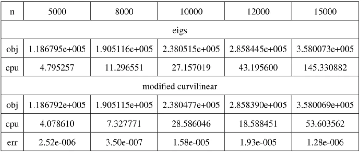
In this section, we illustrate the computational advantage of Algorithm 2 in the linear eigenvalue problem (2.2). We compare Algorithm 2 against the Matlab function “eigs” in a number of test matrices. We first implement the algorithm in a few randomly gen-erated dense matrices Σ. In Table 2.1, n varies from 5000 to 15000, and p=6 (we
calculate the sum of the 6 largest eigenvalues). In this table, “obj” denotes the optimal value of the objective function, “cpu” denotes the CPU time, “err” denotes the relative error between the results from eigs and modified algorithm (Algorithm 2). We see that the two algorithms have similar performance whennis small, but whenn>10000, mod-ified curvilinear algorithm (Algorithm 2) is significantly faster than eigs. In Table 2.2, we fix n=10000 and vary p. We see that Algorithm 2 is faster, especially when pis relatively small (p=1).
Table 2.1: Comparision of eigenvalue calculation on random matrices with p = 6
n 5000 8000 10000 12000 15000
eigs
obj 1.186795e+005 1.905116e+005 2.380515e+005 2.858445e+005 3.580073e+005
cpu 4.795257 11.296551 27.157019 43.195600 145.330882
modified curvilinear
obj 1.186792e+005 1.905115e+005 2.380477e+005 2.858390e+005 3.580069e+005
cpu 4.078610 7.327771 28.586046 18.588451 53.603562
err 2.52e-006 3.50e-007 1.58e-005 1.93e-005 1.28e-006
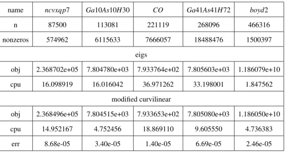
In our second experiment, we apply both methods to 5 large sparse matrices (n≥ 80000) from the UFL Sparse Matrix Collection (Davis and Hu 2011). We compute the 6 largest eigenvalues and present the results in Table 2.3. In this table, “nonzeros” denotes the number of non-zero entries in the sparse matrices. We see that Algorithm 2 is competitive in most problems, and significantly faster than “eigs” on problems such
Table 2.2: Comparision of eigenvalue calculation on random matrices with n = 10000
p 1 3 5 7 9
eigs
obj 3.984335e+004 1.193378e+005 1.985642e+005 2.774991e+005 3.562744e+005
cpu 14.305161 28.298328 23.106653 27.356422 27.338908
modified curvilinear
obj 3.984330e+004 1.193376e+005 1.985640e+005 2.774922e+005 3.562709e+005
cpu 5.807126 19.767615 12.661969 16.551770 19.016399
err 1.10e-006 1.37e-006 1.10e-006 2.47e-005 9.82e-006
as “Ga10As10H30” and “Ga41As41H72”. However, “eigs” has excellent performance on “boyd2” (less than 2 seconds), and is dramatically faster than Algorithm 2. When a matrix has special structures, “eigs” is able to capture them to reduce the computation time.
Table 2.3: Comparision of eigenvalue calculation on real sparse matrices from Sparse Matrix Collection - CISE.UFL
name ncvxqp7 Ga10As10H30 CO Ga41As41H72 boyd2
n 87500 113081 221119 268096 466316
nonzeros 574962 6115633 7666057 18488476 1500397
eigs
obj 2.368702e+05 7.804780e+03 7.933764e+02 7.805603e+03 1.186079e+10 cpu 16.098919 16.016042 36.971262 33.198001 1.847562
modified curvilinear
obj 2.368496e+05 7.804515e+03 7.933653e+02 7.805080e+03 1.186050e+10
cpu 14.952167 4.752456 18.869110 9.605550 4.736383
2.2
Algorithm for Sparse Principal Component Analysis
2.2.1
Hybrid Principal Component Analysis (HPCA)
In the previous section, we have shown that Algorithm 2 is an efficient method in solving the linear eigenvalue problem (2.2), especially for high dimensional matrices. Nonethe-less, it only calculates the eigenvalues, but not the eigenvectors. However, it can improve the efficiency of an existing method for sparse principal component analysis.
Sparse principal component analysis (SPCA) has been extensively studied for the last few decades. In this work, we formulate the problem as follows:
max X∈Rn×ptr(X T ΣX)−ρ|X| s.t. |XiTΣXj| ≤∆i,j, XTX =I, (2.6)
where∆i,j≥0(i6= j)are tuning parameters for the correlation of X, and ρ >0 is the penalized parameter of sparsity. This sparse PCA formulation maintains the following three properties of the standard PCA: (1) maximal total explained variance, (2) uncorre-lation of principal components, (3) orthogonality of loading vectors.
As a recent work, Lu and Zhang (2012) give an augmented Lagrangian method (Al-gorithm 3) for solving a generalization of (2.6). The problem is written as
min
X∈Rn×pf(X) +P(X)
s.t. gi(X)≤0, i=1, . . . ,m,
hj(X) =0, j=1, . . . ,p, (2.7)
smooth.
Algorithm 3:Augmented Lagrangian method for (2.7)
1 Setk=0,λ0, µ0,ρ0>0,τ>0,σ >1;
2 Find an initial pointXinit0 and a constantϒ>max{f(Xf eas),Lρ0(X
0
init,λ0,µ0)};
3 whiletruedo
4 Find a candidate solutionXkfor the subproblem
min Xk Lρk(X k init,λk,µk):=w(Xk) +P(Xk) wherew(Xk) = f(Xk) + (k[λk+ρkg(Xk)]+k2− kλk2)/(2ρk) +µkh(Xk) +ρkkh(Xk)k2/2;
5 Update Lagrange multipliers
λk+1= [λk+ρkg(Xk)]+, µk+1=µk+ρkh(Xk)
Setρk+1=max{σ ρk,kλk+1k1+τ,kµk+1k1+τ};
6 If maxi6=j[|XiTΣXj| −∆i,j]+≤εI, max|XTX−I| ≤εE, and
|Lρ(X,λ,µ)−f(X)|/max(|f(X)|,1)≤εOthen stop; Otherwise,k=k+1 and continue;
7 end
Notice that (2.6) is a special case of (2.7). In Lu and Zhang (2012), they directly ap-ply Algorithm 3 , which they called “Alspca”, to (2.6). They have shown that it properly controls the orthogonality and correlation of the components X while maintaining the sparsity. However, Algorithm 3 uses the standard SVD decomposition to find an initial point, which is not computationally efficient, and sometimes even intractable in high dimensional matrices. Thus, we incorporate Algorithm 2 into Algorithm 3 to solve (2.6) for high dimensional matrices. That is, we use Algorithm 2 to get a feasible starting
pointXinit0 for Algorithm 3 in our high dimensional matrix computation. Our final hy-brid algorithm is listed as follows:
Algorithm 4:A hybrid algorithm for high dimension matrix (“HPCA”)
1 Use Algorithm 2 to find an plausible initial point forXinit0 ; 2 UseXinit0 in Algorithm 3 to find the optimal pointX.
The idea of HPCA is to quickly find the orthogonal componentsXusing Algorithm 2 as an initial point, and then use Algorithm 3 to reduce the correlations ofX, increase the sparsity ofX, while maintaining their orthogonality.
2.2.2
Numerical Results of HPCA in Sparce Principal Component
Analysis
In this section, we explore the numerical performance of HPCA (Algorithm 4) in sparse PCA (2.6) using randomly generated matrices. In particular, we compare HPCA against Alspca and a most commonly used SPCA method, the generalized power methods (GPower) (Journ´ee et al. 2010), w.r.t. total explained variance, correlation of PCs, orthogonality of loading vectors, and computation times. We use two types of gen-eralized power methods, single-unit SPCA vial1penality (“GPowerl1”) and single-unit SPCA vial0penality (“GPowerl0”). As mentioned by Lu and Zhang (2012),tr(XTΣX)
in (2.6) basically equals the total explained variance of the first p PCs. However, the PCs found by SPCA are not perfectly uncorrelated, andtr(XTΣX)can overestimate the
total explained variance by the PCs due to the overlaps of the individual variances. As a result, Lu and Zhang (2012) introduced the adjusted total explained variance and the
cumulative percentage of adjusted variance (CPAV) for sparse PCs: Ad jVar=tr(XTΣX)− r
∑
i6=j (XiTΣXj)2, CPAV =Ad jVar/tr(Σ), (2.8) In our experiments, we use CPAV as a metric for measuring the total explained variance. In the first one, we try to find the first 6 sparse PCs with the average percentage of zero loadings to be approximately around 80% (80% sparsity). To achieve this, the tuning parameterρ for Problem (2.6) and the parameters for the GPower methods are chosenproperly. The test set includes 1000 full-rank random matrices. The results in Table 2.4 correspond to the matrix with size 200×200 and 1000×1000 separately. In this table, “sparsity” measures the number of zero loadings averaged over all instances. The third row “Ortho(Mean)” gives the average amount of orthogonality of the loading vectors, which is measured by the maximum absolute angles formed by all pairs of loading vec-tors. Larger values in this row imply better orthogonality. The fourth row “Ortho(Std)” gives the corresponding standard deviation. The average maximum correlation between all pairs of loading vectors is given in row five (“Corr(Mean)”), and the corresponding standard deviation is given in row six (“Corr(Std)”). The rows seven and eight (“CPAV (Mean)”, “CPAV (Std)”) give the average CPAV (defined in (2.8)) and its standard devi-ation. The average cpu time and the corresponding standard deviation are given in the last two rows.
From Table 2.4, we see that HPCA and Alspca give nearly identical results, while HPCA is more computationally efficient. Specifically, HPCA spends roughly 20% less computing time in the 200×200 matrix test, and 25% less time in the 1000×1000 ma-trix test. HPCA is also more stable than Alspca in computation time with a smaller stan-dard deviation in both size of matrices. Also, Alspca and HPCA obtain almost uncorre-lated sparse PCs and nearly orthogonal loading vectors, which outperforms the GPower methods. Alspca and HPCA are also more stable in controlling the correlation and or-thogonality, as both methods have smaller standard deviations than GPower. In terms of
Table 2.4: Comparision of SPCA methods on randomly generated full-rank ma-trices with p=6
Method
200×200 1000×1000
GPowerl1 GPowerl0 Alspca HPCA GPowerl1 GPowerl0 Alspca HPCA
Sparsity 0.8008 0.8035 0.8099 0.8007 0.8039 0.8066 0.8091 0.8099 Ortho(Mean) 87.134 87.327 89.991 89.987 86.433 86.730 90.000 89.997 Ortho (Std) 0.533 0.582 0.022 0.030 0.404 0.386 0.022 0.023 Corr (Mean) 0.062 0.066 0.026 0.025 0.049 0.043 0.015 0.014 Corr (Std) 0.018 0.018 0.004 0.004 0.010 0.009 0.002 0.002 CPAV%(Mean) 4.972 4.881 4.982 4.982 1.759 1.923 1.950 1.953 CPAV%(Std) 0.007 0.008 0.010 0.010 0.022 0.019 0.011 0.011 CPU (Mean) 0.063 0.054 5.166 3.915 0.655 0.514 53.623 38.915 CPU (Std) 0.012 0.008 0.518 0.396 0.096 0.083 5.125 3.696
CPAV, there are no significant differences among these three methods. Gpower method, however, is extremely efficient in computation time. This is mainly because Gpower solves two unconstrained differentiable maximization problems, instead of (2.6), forl1
penality andl0penality respectively, max x∈Rn √ xTΣx−γkxk1, max x∈Rnx T Σx−γkxk0, (2.9) whereγ >0 is the sparsity controlling parameter. GPower does not have any constraint
on the correlation and orthogonality of PCs, and the resulting variances of the first few PCs are not ordered either.
In the second experiment, we randomly generate 1000 200×200 and 1000 1000× 1000 matrices with rank 10 and fixed eigenvalues 100, 89.2, 78.4, 67.7, 56.9, 46.1, 35.3, 24.6, 13.8, 3.0. We set p=6 and 80% sparsity, and present the results in Table 2.5. We see that GPower has substantially higher maximum correlation than both Alspca and HPCA. This is because Gpower does not have constraints on the correlation of loading vectors, and is hence sensitive to the rank of the test matrices. GPower also has smaller
Table 2.5: Comparision of SPCA methods on randomly generated low-rank ma-trices with p=6
Method
200×200 1000×1000
GPowerl1 GPowerl0 Alspca HPCA GPowerl1 GPowerl0 Alspca HPCA
Sparsity 0.8085 0.8082 0.8073 0.8073 0.8070 0.8097 0.8025 0.8010 Ortho(Mean) 85.098 85.262 89.968 89.955 87.865 87.839 89.945 89.959 Ortho (Std) 1.438 1.242 0.054 0.065 0.686 0.784 0.052 0.053 Corr(Mean) 0.637 0.684 0.159 0.158 0.710 0.750 0.026 0.025 Corr (Std) 0.095 0.099 0.047 0.043 0.071 0.082 0.002 0.002 CPAV%(Mean) 40.517 40.821 42.891 42.892 32.181 33.303 49.303 49.303 CPAV%(Std) 0.281 0.302 0.118 0.114 0.215 0.194 0.119 0.118 CPU (Mean) 0.008 0.007 3.493 2.512 0.197 0.170 74.294 58.961 CPU (Std) 0.004 0.004 0.411 0.238 0.030 0.022 8.125 5.996
CPAV and orthogonality than Alspca and HPCA. When we increase the matrix size from 200×200 to 1000×1000, GPower has a smaller the average CPAV (from 40% to 33%) while Alspca and HPCA have a higher one (from 43% to 49%). In terms of computation time, GPower is more efficient than Alspca and HPCA, which we have discussed in the previous experiment. Combining Table 2.4 with Table 2.5, we find that Alspca and HPCA spend more time to deal with low rank matrices than with full rank ones, while the opposite is true for GPower.
2.3
Application of HPCA in Equity Statistical Arbitrage
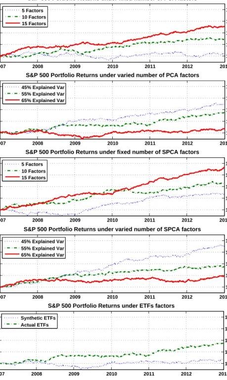
We now apply HPCA (Algorithm 4) to a statistical arbitrage strategy where we trade a portfolio of stocks against market factors, which are defined using the standard PCA, or the corresponding sector exchange-traded funds (ETFs). We extend the work of Avel-laneda and Lee (2010) to define market factors using HPCA, and examine their
perfor-mance from 2007 to 2013.
2.3.1
Problem Formulation
In statistical arbitrage, we decompose the stock return into two parts: the return that can be explained by some common market factors, and the idiosyncratic return. The id-iosyncratic part can be modeled statistically by stationary mean reversion process. This paradigm is based on the assumption of market overreaction, for instance, some stocks are temporarily mispriced with respect to other reference stocks or indices, and open market operations will revert their prices back in a short period of time (Lo and MacKin-lay 1990). The trading strategy for this paradigm is called “pairs-trading” (Avellaneda and Lee 2010). Suppose that stockSand reference securityQin the same industry have similar characteristics, and we expect their returns are tractable with each other. The general decomposition of stock return based on market factors is then
dSt St =β0dt+β1 dQt Qt +dXt, (2.10)
whereSt is the time-series price of the stock,Qt is the time-series price of the reference security respectively, Xt is a stationary mean reverted process, β0 is the time drift, and
β1 is the regression coefficient. In (2.10), Xt is the idiosyncratic part. If β1 is chosen carefully, the mean reverted property ofXt guarantees that the long-short portfolio ofS andQoscillates near its statistical equilibrium. However, it is extremely difficult to find such a pairS andQin practice. Instead, people usually employ an extension of (2.10), called “generalized pairs-trading”,
dSt St =β0dt+ n
∑
j=1 βjF (j) t +dXt, (2.11)2.3.2
Methods for Modeling Market Factors
The first method for finding market factors in (2.11) is to choose corresponding sector ETFs. ETFs are investment assets traded on stock exchanges that provide exposure to a certain sector. Since the late 1990s, more and more investors choose ETFs to diver-sify their portfolio because of the following reasons: (1) ETFs provide straightforward tradable access to an individual sector or industry, (2) nowadays there are thousands of ETFs available in the worldwide markets, (3) ETFs are very liquid.
From the perspective of statistical arbitrage, it is advantageous to choose ETFs as market factors in (2.11). The first reason is that ETFs allow a stock to be traded directly against corresponding sector ETFs when the stock price diverges from the statistical equilibrium, hence it is straightforward to incorporate ETFs into the model. Secondly, it is intuitive to interpret the factor loadings when we choose ETFs as market factors. Nevertheless, selecting ETFs requires some prior knowledge of the economy and indus-try, and most ETFs have the priori capitalization bias, that is, ETFs holdings give more weight to large capitalization companies. Also, ETFs are correlated, which brings some redundancies into the model. These issues push people towards some other approaches.
As a fundamental tool of data analysis, principal component analysis (PCA) can also be applied to the correlation matrix of the stock returns to extract market factors in (2.11). Avellaneda and Lee (2010) justified that we can consider principal components as long-short portfolio of industry sectors. We now describe the procedure of deriving the market factors. Assume that{Si,t}, i=1, . . . ,N, t=0, . . . ,M are adjusted closing stock prices forN stocks over the pastM time periods. The stock price return and the standardized price return are
Ri,t= Si,t−Si,t−1 Si,t−1 and Yi,t= Ri,t−R¯i ¯ σi , (2.12)
where ¯ Ri= 1 M M
∑
t=1 Ri,t and σ¯i2= 1 M−1 M∑
t=1 (Ri,t−R¯i)2. (2.13) We then generate theN×Ncorrelation matrix of empirical returns with the(i,j)thentry to be ρi,j= 1 M−1 M∑
t=1 Yi,tYj,t. (2.14)PCA then extracts the eigenvalues and eigenvectors of the correlation matrix (2.14), denoted by λj and v(j) = (v(1j), . . . ,v(Nj)), j =1, . . . ,N. Without loss of generality, we assume{λj}Nj=1 are in a decreasing order, and the eigenvectors{v(j)}Nj=1 of the corre-lation matrix are tied with the market factors in the following way: the entries of an eigenvector corresponds to the weights in a particular stock. If we scale the weights by the volatility of the stock, we can view each eigenvector as a portfolio that holds weights in each stock (Avellaneda and Lee 2010). The weights are
Q(ij)= v (j) i ¯ σi . (2.15)
Incorporating the stock return, we get the eigenportfolio return series or market factor return series, Ft(j)= N
∑
i=1 v(ij) ¯ σi Ri,t. (2.16)From (2.16) we conclude that each stock return can be decomposed into the projection on market factors and idiosyncratic residuals, as in (2.11).
PCA delivers a set of orthogonal market factors. Compared with the ETFs approach, it does not require any specific prior information about the economy. However, PCA has its own drawback – since each eigenportfolio is a linear combination of all stock returns, and the loadings are usually nonzero, it is often difficult to interpret the derived eigen-portfolios. Several previous authors have dealt with this issue. For instance, Laloux
et al. (2000) linked the first eigenportfolio, which corresponds to the eigenvector with the largest respective eigenvalue, with the market, or equivalently, a generalized index on the market. Avellaneda and Lee (2010) noted an interesting phenomenon: when we rank the coefficients of the eigenvectors in a decreasing order, different company stocks presented by adjacent coefficients tend to be in the same industry. But this is not neces-sary true for some noisy eigenvectors.
To improve the interpretability of PCA, we use SPCA as an alternative. The proce-dure for deriving the market factors is exactly the same as with PCA. The only difference is to use SPCA instead of PCA to extract eigenvalues and eigenvectors from correlation matrix (2.14). In our implementation of SPCA, we use HPCA (Algorithm 4) defined in Section 2.2.1.
Both PCA and SPCA reduce the dimension of original dataset by projecting along the orthogonal eigenvectors, which represent the maximum variance of the data in each direction. We choose the number of eigenvectors using two criteria: (1) A fixed number of eigenvectors, in which case the total variance explained changes every time, (2) flex-ible number of eigenvectors, in order to keep a specific total variance explained every time. We apply both criteria in Section 2.3.4
2.3.3
Trading Signals and Arbitrage Strategy
In the previous section, we have discussed three methods (ETFs, PCA, SPCA) to find market factors {Ft(j)} in (2.11). Now we follow the approach in Avellaneda and Lee (2010) to generate trading signals, which can be used for trading against any market factors.
We first compute the regression model for each stocki,i=1, . . . ,N, using a window ofMdays, Ri,t=βi,0+ n
∑
j=1 βi,jF (j) i,t +εi,t, t=1, . . . ,M, (2.17) whereRi,t is the return of stockiat timet, βi,0is the drift, {F(j)
t }nj=1and{βi,j}nj=1are its market factors and the corresponding regression coefficients for stocki, andεi,tis the residual of stockiat timet.
We then generate the cumulative residual returns, which is a discrete time proxy for the residual time-series process. We assume that this time series follows anAR(1)
process, Xi,t= t
∑
k=1 εi,k, t=1, . . . ,M. (2.18) Xi,t+1=ai+biXi,t+ζi,t+1. t=1, . . . ,M−1. (2.19) For each stock we then compute an “s-score” (Avellaneda and Lee 2010), modeling the distance of the residual returns from the statistical equilibrium. Based on this score, we identify when the stock is away from the equilibrium, and enter the mean reversion position to restore the equilibrium. The s-score for stockiat timet is defined bysi,t = Xi,t−mi σi,t , (2.20) where mi= ai 1−bi and σi,t= s Var(ζi,t) 1−b2i . (2.21)
We then open or close trades as follows:
• long to open the position ifsi,t<−1.25, • short to open the position ifsi,t>1.25,
• close the short position ifsi,t<0.75, • close the long position ifsi,t>−0.5.
The cutoff values 1.25, 0.75, and 0.5 are determined empirically based on the simu-lated strategies from 2000 to 2004 (Avellaneda and Lee 2010). We use these values consistently across all three methods for modeling market factors.
2.3.4
Backtesting Results
To evaluate the performance of an arbitrage strategy we backtest it using the trading signals from Jan 1, 2007 to Dec 31, 2013. We determine the tradable set of stocks on the starting datedbased on the following criteria:
• The stock must be a member of the reference index on dated
• The market capital on dated must be greater than certain threshold, e.g. $1bn
On date d we open new positions only on stocks in the tradable set. We define a re-balance period, say after 60 days, when we recompute the tradable set from the most recent reference index constituents. In between these rebalance periods, the tradable set remains constant. We examine the returns of each approach in Section 2.3.2 on a port-folio of $100 over the past 6 years, from 2007 to 2013. The portport-folio consists of stocks from the constituents ofS&P500.
There are two alternative implementations for ETFs approach, (1) synthetic ETFs comprised of 15 capitalization-weighted industry indices (Avellaneda and Lee 2010); (2) actual ETFs in the market. For PCA and SPCA, we set the number of market factors in two ways, (1) fixed, e.g., 5, 10, or 15; (2) flexible, explaining 45%, 55%, or 65% of
2007 2008 2009 2010 2011 2012 2013 100 102 104 106 108
S&P 500 Portfolio Returns under fixed number of PCA factors
Year Dollar($) 5 Factors 10 Factors 15 Factors 2007 2008 2009 2010 2011 2012 2013 100 102 104 106 108
S&P 500 Portfolio Returns under varied number of PCA factors
Year Dollar($) 45% Explained Var 55% Explained Var 65% Explained Var 2007 2008 2009 2010 2011 2012 2013 100 102 104 106 108
S&P 500 Portfolio Returns under fixed number of SPCA factors
Year Dollar($) 5 Factors 10 Factors 15 Factors 2007 2008 2009 2010 2011 2012 2013 100 102 104 106 108
S&P 500 Portfolio Returns under varied number of SPCA factors
Year Dollar($) 45% Explained Var 55% Explained Var 65% Explained Var 2007 2008 2009 2010 2011 2012 2013 100 102 104 106 108
S&P 500 Portfolio Returns under ETFs factors
Year
Dollar($)
Synthetic ETFs Actual ETFs