THE IMPACT OF MISSING LABELS AND OVERLAPPING SOUND EVENTS ON
MULTI-LABEL MULTI-INSTANCE LEARNING FOR SOUND EVENT CLASSIFICATION
Maarten Meire
1, Lode Vuegen
1, Peter Karsmakers
1 1KU Leuven, Dpt. of Computer Science, TC CS-ADVISE,
Kleinhoefstraat 4, B-2440 GEEL, Belgium, [email protected]
ABSTRACT
Automated analysis of complex scenes of everyday sounds might help us navigate within the enormous amount of data and help us make better decisions based on the sounds around us. For this pur-pose classification models are required that translate raw audio to meaningful event labels. The specific task that this paper targets is that of learning sound event classifier models by a set of exam-ple sound segments that contain multiexam-ple potentially overlapping sound events and that are labeled with multiple weak sound event class names. This involves a combination of both multi-label and multi-instance learning. This paper investigates two state-of-the-art methodologies that allow this type of learning, low-resolution multi-label non-negative matrix deconvolution (LRM-NMD) and CNN. Besides comparing the accuracy in terms of correct sound event classifications, also the robustness to missing labels and to overlap of the sound events in the sound segments is evaluated. For small training set sizes LRM-NMD clearly outperforms CNN with an accuracy that is 40 to 50% higher. LRM-NMD does only mi-norly suffer from overlapping sound events during training while CNN suffers a substantial drop in classification accuracy, in the or-der of 10 to 20%, when sound events have a 100% overlap. Both methods show good robustness to missing labels. No matter how many labels are missing in a single segment (that contains multiple sound events) CNN converges to 97% accuracy when enough train-ing data is available. LRM-NMD on the other hand shows a slight performance drop when the amount of missing labels increases.
Index Terms— Multi-label learning, multi-instance learning, weak labels, non-negative matrix deconvolution, convolutional neu-ral networks, overlapping sound events, polyphonic classification, sound event classification.
1. INTRODUCTION
We are surrounded by complex acoustic scenes made up of many potentially overlapping sound events. For example, in a busy street we may hear engine sounds in cars, footsteps of people walking, doors opening, or people talking. Large amounts of recorded sound clips are also being uploaded into audio and multimedia collections of clips on the internet, creating an explosive growth in this audio data. In recent years, research into content analysis for complex au-dio has found increasing attention in the research community [1]. It has lead to algorithms based on machine learning that automate the analysis of the complex audio of everyday sounds, to help us nav-igate within the enormous amount of data and help us make better decisions based on the sounds around us.
In this work we specifically focus on the task of learning sound event classifier models by a set of sound segments that contain mul-tiple potentially overlapping sound events and that are labeled with
multiple weak sound event class names. Such setup involves a combination of multi-label and multi-instance learning. Multi-label refers to the fact that a single sound segment has multiple labels. When strong labels are used the labelled sound events are all active for the full (small, e.g. 50ms) sound segment. Weak labelled sound events are active on undefined positions in the considered (larger, e.g. 10s) audio segment. Hence, the learning strategy should have the ability to identify multiple instances that are present within an audio fragment. For example learning sound event models based on YouTube movies that have meta information (that could be automat-ically transformed into some predefined set of class labels) could be considered as a multi-label multi-instance learning task.
The literature concerning the classification of overlapping sounds is mainly divided into two separate streams. Either the over-lapping events are separated first using source separation methods [2, 3] or region extraction methods such as [4] prior to detection or the overlapping events are directly classified via a unifying classfi-cation scheme [5, 6], with the latter being the most successful. In this work we compare two methods that belong to this category. Particularly convolutional neural networks (CNN), potentially with some recurrent layers added, have shown good performance with respect to the considered task [5, 7]. In [8] the authors developed a convolutive modeling technique that combines a sound source sepa-ration strategy based on non-negative matrix devonvolution (NMD) with weak supervision to enable the option to perform classifica-tion. In this paper we will compare both methods not only in terms of classification accuracy but also in terms of robustness to missing labels and the amount of overlap of sound events that are present in the sound segments used during the learning stage.
The literature concerning missing labels in weak labelled data is rather limited. While research into noisy labels has recently been growing [9, 10], the impact of missing labels specifically has not yet been investigated to the best of our knowledge. This is backed up by the statement in [11] that the theme of noisy labels was completely missing from the literature.
This paper is organized as follows. In Section 2 we briefly intro-duce the two methods that are being compared. Section 3 describes the data set that was used and the experimental setup. The results are discussed in Section 4. Final conclusions and future directions are given in Section 5.
2. METHODS 2.1. Non-negative Matrix Deconvolution
NMD is an extension of non-negative matrix factorization (NMF) and is capable of identifying components with a temporal struc-ture [12, 13]. The main objective of NMD is to decompose an all-positive observation data matrixY[o]
∈ RB×F
time-frequency magnitude spectrogram in case of acoustic processing, into the convolution between a set of temporal basis matricesA[o]
t ∈
RB×L
≥0 , witht∈[1, T], and its activation pattern over timeXL≥×0F. The general form of NMD is expressed by
Y[o] ≈Ψ[o]= T X t=1 A[o] t (t−1) − →X , (1) whereΨ[o] ∈RB×F
≥0 denotes the reconstructed data and
t
−→
(·)a ma-trix shift oftentries to the right. Columns that are shifted out at the right are discarded, while zeros are shifted in from the left. The complete set of basis data, i.e. also called ’dictionary’ or ’ sound-book’ is described by combining all temporal basis matricesA[o]
t
into a global three-way tensorA[o]
∈RB×L×T
≥0 . Eachl-th slice of A[o]then contains the temporal basis data of thelth-component over
timetand can be interpreted as one of the additive time-frequency
elements describing the underlying structure inY[o].
The general form of NMD given by Equation 1 factorizes the observations in a blind fashion. In [8] we have proposed an exten-sion to NMD, called low-resolution multi-label non-negative matrix deconvolution (LRM-NMD), where both the observation data and the available labelling information are used during the factorization process. More specifically, let us assume thatY[o]is supported by a multi-label vectory[s]
∈ {0,1}C, withCdenoting the number
of classes, indicating the sound events that have occurred without describing beginnings nor endings. In the other words weak labels are employed. The objective of LRM-NMD is still to decompose Y[o]as is given in Equation 1 but with respect to
y[s]
≈ψ[s]=A[s]X1, (2) withA[s]
∈ {0,1}C×Lacting as a labelling matrix forA[o]and1 being an all-one column vector of lengthF. Hence, the cost
func-tion of LRM-NMD is expressed by min A[o],A[s],X J X j=1 h D(Y[jo]kΨ[jo]) +λkXjk1+ηD(y[js]kψ [s] j ) i , (3)
whereD(vkw)denotes the Kullback-Leibler divergence between vandw,λbeing the sparsity penalty parameter andηthe trade-off parameter between the observation data and the labelling infor-mation. The cost function can be minimised using the method of multiplicative updates as discussed in [8]. LRM-NMD favours de-compositions that have a balanced performance in terms of recon-struction error and classification performance. More specifically, LRM-NMD encourages that the sound events in segmentY[o], la-belled byy[s], are described by a linear combination of a subset of sound book elements inA[0]each assigned to a specific sound event class by the labelling matrixA[s]. Two crucial advantages of LRM-NMD are: a) that it can deal directly with overlapping sound events in the observation data, i.e. because of the additive behaviour due to the non-negativity constraint, and b) that not all events in an acous-tic segment must be labelled and thus that it can cope with missing labels enabling a semi-supervised learning strategy that learns the model parameters from both labelled and unlabelled data.
Classifying an unseen sample is done by decomposing the test data under the fixed learned basis dataA[o]and performing a global average pooling on the corresponding activationsX.
2.2. Convolutional Neural Network
Convolutional neural networks (CNNs) have become the current state-of-the-art solution for many different machine learning tasks and are already widely discussed in the literature. CNNs usually consist of several pairs of convolutional and pooling layers as a fea-ture extractor. The extracted feafea-tures are usually flattened using a flatten layer and are then followed by one or more fully connected layers that act as a classifier.
In this study we used a basic CNN architecture, using the afore-mentioned layers. To accommodate for variable sized input frames, we changed the flatten layer to a global average pooling layer. This change allows training on segments with a different size compared to those that are being used in the testing phase. While we could train on different length segments, we padded all segments to the length of the longest segment during training for batching purposes. This padding is done, for each mel band, by sampling from a nor-mal distribution with the mean and standard deviation derived from the considered mel band values from the training data.
3. EXPERIMENTAL SETUP 3.1. Dataset
Both methods are validated using the publicly available NAR-dataset. This dataset contains a set of real-life isolated domestic audio events, collected with a humanoid robot Nao, and is recorded specifically for acoustic classification benchmarking in domestic environments [14, 15]. In total 42 different sound classes were recorded and can be categorised into ’kitchen related events’, ’ of-fice related events’, ’non-verbal events’ and ’verbal events’. The verbal events are not used in this research which reduces the dataset to a total of 20 sound classes each containing 20 or 21 recordings.
The training, validation and test sets are created by randomly sampling instances from the NAR-dataset with a ratio of50%for training,25%for validation and25%for testing. The training and validation sets are further processed into so-called acoustic observa-tion segments for the multi-instance multi-label learning task. More specifically, the acoustic segments are generated by randomly draw-ing five events, sortdraw-ing them with increasdraw-ing time duration, and combining them into a single stream with0%, 25%, 50%, 75%
and 100%overlap1. In total 10000 training and 2000 validation segments were generated per degree of overlap. The test set was not altered since the envisioned task of the experiments later is sim-ply a classification problem. The previous process was repeated four times resulting in a final dataset containing 4 folds each made up of 10000 training segments, 2000 validation segments, and 100 isolated test samples (5 per sound class) for classification.
3.2. Features
The so-called mel-magnitude spectrograms [16] have shown to be a good choice of acoustic features having the properties of non-negativity and approximate additivity. The mel-magnitude spectro-grams that span 40 bands are computed using a Hamming window with a frame length of 25 ms and a frame shift of 10 ms as proposed in [17]. The used filter bank is constructed such that the begin fre-quency of the first filter and the end frefre-quency of the last mel-1The amount of overlap is defined by the amount of overlapping samples
between two successive events, based on the first event. Special case is 100%where all events in the acoustic segment have the same onset time.
filter correspond to the frequency range of the microphone, i.e. 300 Hz and 18 kHz.
3.3. Experiments
In this paper two main experiments were carried out. The first ex-periment investigates the influence of the number of training seg-ments (ntr) on the classification performance of LRM-NMD and
CNN for different degrees of assigned labels (nlbl). The number of
training segments are increased offline from 50 to 10,000 and the amount of assigned labels varies betweennlbl = 1(4 missing
la-bels per segment) andnlbl= 5(no missing labels). The second
ex-periment investigates the influence of overlapping sound events on the classification performance of LRM-NMD and CNN for a fixed number of training segments. The investigated degrees of overlap (novl) vary betweennovl = 0%andnovl = 100%. The amount
of assigned labels varies again in the rangenlbl = {1,2,3,4,5}.
In both experiments, the objective is to predict a single label for an event while training on multi-label segments.
The set of dictionary elements inA[o]for LRM-NMD was ini-tialized with one example per sound class and one additional dic-tionary element with small positive noise for acoustic background modelling. Hence, the overall dimensions of A[o] are B = 40,
L = 21, andT = 40. The labelling matrixA[s]was initialised by an identity matrix augmented with an all zeroClong column vector for the background dictionary element. The used hyperparameters areλ= 5andη= 5and where selected from the results in [8].
The network used for CNN starts with 3 convolutional layers using (5,5) filter shapes and 64 filters, similar to what was proposed in [5], each convolutional layer is followed by a batchnormalization [18] layer, a relu activation and a pooling layer. The pooling layers used maxpooling with (5,1), (3,1), (2,1) as shapes respectively. Af-ter these layers a globalaveragepooling layer is added, followed by a hidden fully connected layer of 64 neurons, with a relu activation, and an output layer of 20 neurons, the same amount as the number of output classes. Between all convolutional layers dropout [19] is used with a drop rate of 0.5. During training the output layer has a sigmoid activation, due to the multi-label nature of this problem, and during inference this activation is changed to a softmax since a single label is required. Since this is a multi-label problem with binarized labels, binary-crossentropy is used as the loss function. Adam was used as optimizer with a learning rate of 0.001.
4. RESULTS
In this section the results of both experiments are discussed. Firstly, we will discuss the effect of missing labels and the amount of train-ing samples on the performance of both methods. Secondly, we will discuss the impact overlap in training segments has in both meth-ods. Finally, while this is not the main focus of this study, we will do a short comparison of our results to the results of other studies which used the NAR-dataset.
4.1. Missing labels
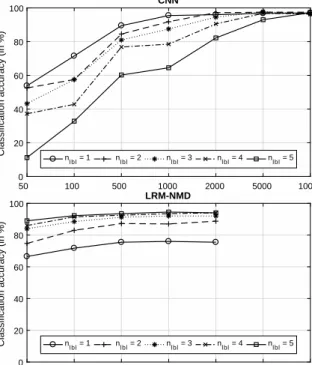
The results of this experiment for CNN and LRM-NMD are pre-sented in Figure 1. The LRM-NMD model was trained with at most
ntr = 2000, while the CNN was trained up tontr = 10000,
how-ever we assume that the results of LRM-NMD will not have a large improvement with a higherntrbased on the trend in the results.
From these results we can see that LRM-NMD substantially outperforms CNN in cases where there is little data available. The latter is mainly the result of the exemplar based initialization of LRM-NMD resulting in a bootstrapped model structure. At
ntr = 50, CNN achieves accuracies ranging from 53.8±6.1%
to11.2±8.2%for 5 labels and 1 label, respectively. In
compari-son, for the samentr, LRM-NMD achieves accuracies ranging from 89.0±3.4%to66.5±4.4%.
When considering the results when more training segments are added, we can see that CNN begins to achieve similar accuracies as LRM-NMD when a few labels are missing. Atntr = 1000, CNN
achieves accuracies ranging from95.5±1.1%to64.5±9.1%for 5 labels and 1 label, respectively. For the samentr LRM-NMD
achieves accuracies ranging from94.5±2.5% to 76.0±2.4%. These numbers confirm our statement that CNN achieves similar ac-curacies as LRM-NMD when few labels are missing, if more train-ing data is added.
If further training data is added, sontr = 10000, we see that
the achieved accuracies converge around97%across allnlbl. From
this we can state that CNN sligthly outperforms LRM-NMD, if a large amount of training data is available. Note that compared to CNN, LRM-NMD uses less model parameters and has no non-linear modeling option available.
Another observation is that while LRM-NMD has a good per-formance for a smallntr, it does not improve as much compared
to CNN whenntr increases. Note that the LRM-NMD
hyperpa-rameters i.e. ηandλ, were selected and kept fixed in a model se-lection procedure in which all labels were present for each training segment (hence no missing labels). This choice is probably sub-optimal since the amount of provided labels influences the balance between the supervision and reconstruction error terms in 3. 4.2. Overlap of events in segments
In this experiment we usedntr = 10000for CNN andntr = 500
for LRM-NMD. These amounts were chosen based on the classifi-cation accuracies and the time needed to train the models. For CNN the accuracies converged forntr = 10000and for LRM-NMD they
started stagnating forntr= 500. The results of the experiment are
presented in Figure 2.
Fornovl= 0%we can see that CNN outperforms LRM-NMD,
this can be attributed to the increase inntr, as described in 4.1.
CNN is converged around 97% accuracy, while the accuracies achieved by LRM-NMD range from93.5±3.1%to75.5±3.9%.
Atnovl = 50%the accuracies achieved by CNN start to
di-verge slightly, ranging from96.8±1.3%to94.5±2.7%. In com-parison, LRM-NMD achieves accuracies ranging from92.5±3.7%
to66.3±1.5%. At this point CNN still outperforms LRM-NMD. However, when we look atnovl= 100%, we see that CNN has
a drop in classification accuracy. The classification accuracy ranges from80.2±1.3%to67.5±5.7%, while the classification accuracy
of LRM-NMD ranges from90.0±3.2%to67.3±7.5%. From these results, we conclude that for up tonovl = 75%
CNN outperforms LRM-NMD. However, if novl gets closer to
100%, LRM-NMD starts to achieve higher accuracies than CNN. A possible explanation for this could be that, due to the nature of the generation of the overlap in the segments, the filters of CNN are smaller than the non-overlapping part of the events for less than 100% overlap. This could lead to the CNN still being able to rec-ognize the events in this non-overlapping area, while the rest of the event is overlapped with the next event.
50 100 500 1000 2000 5000 10000 0 20 40 60 80 100
Classification accuracy (in %)
CNN
n
lbl = 1 nlbl = 2 nlbl = 3 nlbl = 4 nlbl = 5
50 100 500 1000 2000 5000 10000 Amount of training segments (ntr)
0 20 40 60 80 100
Classification accuracy (in %)
LRM-NMD
n
lbl = 1 nlbl = 2 nlbl = 3 nlbl = 4 nlbl = 5
Figure 1: The obtained classification results for CNN and LRM-NMD in function of the number of training segments (ntr) and the
number of labelled events per segment (nlbl). Note thatntr = 5000
andntr = 10000are not evaluated for LRM-NMD due to the
com-putational complexity of the multiplicative updates and the stagna-tion of the results.
An important aspect to note here is that the CNN had more training data. With a smaller training set size, the performance of CNN is worse.
4.3. Comparison with other papers
This paragraph compares the results of this study with other studies using the NAR-dataset. For this comparison we used the best results achieved in the studies, i.e. 96.0% in [14], 97.0% in [15], 98.36% in [20], and 100.0% in [21], and for LRM-NMD and CNN we used the best results with no missing labels and 0% overlap, 94.5% and 97.0% respectively. Note that in the other studies the learning is done using single strong labels, while in this study multi weak la-bels were used. This makes a direct comparison unfair due to the different natures of learning, however, based on the results, we can cautiously state that we approach state-of-the-art performance.
5. CONCLUSION
In this work two experiments that compare the classification per-formance of a CNN-based and a LRM-NMD-based approach for acoustic event classification using weakly multi-labelled data were performed.
The first experiment was done to examine the influence of the amount of training data on the classification performance for dif-ferent amounts of missing labels. In this experiment we observed that for a low amount of data LRM-NMD clearly outperforms CNN
100% 75% 50% 25% 0% 0 20 40 60 80 100
Classification accuracy (in %)
CNN
n
lbl = 1 nlbl = 2 nlbl = 3 nlbl = 4 nlbl = 5
100% 75% 50% 25% 0% Degree overlap (novl)
0 20 40 60 80 100
Classification accuracy (in %)
LRM-NMD
n
lbl = 1 nlbl = 2 nlbl = 3 nlbl = 4 nlbl = 5
Figure 2: The obtained classification results for CNN and LRM-NMD in function of the degree of overlap (novl) and the number of
labelled events per segment (nlbl). Note that CNN uses the setting
ofntr= 10000and LRM-NMDntr = 500.
with an accuracy that is 40 to 50% higher, on each amount of miss-ing labels. However, if enough trainmiss-ing data is added, CNN slightly outperforms LRM-NMD and converges to 97% accuracy for all amounts of missing labels. Results from this experiment indicate that, with large training set sizes and with a uniform probability of a label being absent over classes, missing labels have a very limited effect on the classification performance of a CNN.
In the second experiment we examined the impact of overlap on the classification performance. This experiment was done using
ntr = 500and ntr = 10000for LRM-NMD and CNN
respec-tively which gave the best models in the former experiment for 0% overlap of both approaches. We conclude that for up to 75% overlap CNN outperforms NMD and converges to 97% while LRM-NMD reaches 95% accuracy. However, if the amount of overlap increases further, LRM-NMD starts to outperform CNN, with up to 10% higher accuracies for different amounts of missing labels. In this experiment we have also seen that overlap has a relatively limited impact on LRM-NMD.
In future work we also target to develop a neural network al-ternative to the LRM-NMD algorithm that we proposed in [8]. In this way we can benefit from the modelling flexibility (e.g. the abil-ity to include non-linearabil-ity in the modelling process) that comes with neural networks allowing for several extensions and general-izations, while also keeping the capabilities of LRM-NMD (e.g. be-ing able to use unlabelled data in addition to weak labelled data and the robustness to overlap). Moreover, a more detailed benchmark-ing of the considered methods will be performed on other publicly available data sets.
6. REFERENCES
[1] “DCASE: Detection and classification of acoustic scenes and events,” http://dcase.community/.
[2] T. Heittola, A. Mesaros, T. Virtanen, and M. Gabbouj, “Super-vised model training for overlapping sound events based on unsupervised source separation,” in2013 IEEE International Conference on Acoustics, Speech and Signal Processing, May 2013, pp. 8677–8681.
[3] A. Mesaros, T. Heittola, O. Dikmen, and T. Virtanen, “Sound event detection in real life recordings using coupled matrix factorization of spectral representations and class activity an-notations,” in2015 IEEE International Conference on Acous-tics, Speech and Signal Processing (ICASSP), April 2015, pp. 151–155.
[4] I. McLoughlin, H. Zhang, Z. Xie, Y. Song, and W. Xiao, “Ro-bust sound event classification using deep neural networks,”
IEEE/ACM Trans. on Audio, Speech, and Language Process-ing, vol. 23, pp. 540–552, 2015.
[5] E. C¸akır, G. Parascandolo, T. Heittola, H. Huttunen, and T. Virtanen, “Convolutional recurrent neural networks for polyphonic sound event detection,”IEEE/ACM Transactions on Audio, Speech, and Language Processing, vol. 25, no. 6, pp. 1291–1303, June 2017.
[6] H. Phan, O. Y. Ch´en, P. Koch, L. Pham, I. McLoughlin, A. Mertins, and M. D. Vos, “Unifying isolated and overlap-ping audio event detection with multi-label multi-task convo-lutional recurrent neural networks,” inICASSP 2019 - 2019 IEEE International Conference on Acoustics, Speech and Sig-nal Processing (ICASSP), May 2019, pp. 51–55.
[7] C.-C. Kao, W. Wang, M. Sun, and C. Wang, “R-CRNN: Region-based convolutional recurrent neural network for audio event detection,” inProc. Interspeech 2018, 2018, pp. 1358–1362. [Online]. Available: http://dx.doi.org/10.21437/ Interspeech.2018-2323
[8] L. Vuegen, P. Karsmakers, B. Vanrumste, and H. Van hamme, “Acoustic event classification using low-resolution multi-label non-negative matrix deconvolution,”Audio Engineering Soci-ety (AES), vol. 66, pp. 369–384, 5 2018.
[9] E. Fonseca, M. Plakal, D. P. W. Ellis, F. Font, X. Favory, and X. Serra, “Learning sound event classifiers from web audio with noisy labels,” in ICASSP 2019 - 2019 IEEE Interna-tional Conference on Acoustics, Speech and Signal Processing (ICASSP), May 2019, pp. 21–25.
[10] E. Fonseca, M. Plakal, F. Font, D. P. W. Ellis, and X. Serra, “Audio tagging with noisy labels and minimal supervision,”
arXiv e-prints, p. arXiv:1906.02975, Jun 2019.
[11] A. Shah, A. Kumar, A. G. Hauptmann, and B. Raj, “A Closer Look at Weak Label Learning for Audio Events,” arXiv e-prints, p. arXiv:1804.09288, Apr 2018.
[12] D. Lee and H. Sebastian Seung, “Learning the parts of objects by non-negative matrix factorization,” Nature, vol. 401, pp. 788–91, 11 1999.
[13] P. Smaragdis, “Non-negative matrix factor deconvolution; ex-traction of multiple sound sources from monophonic inputs,” inIndependent Component Analysis and Blind Signal Separa-tion, C. G. Puntonet and A. Prieto, Eds. Berlin, Heidelberg: Springer Berlin Heidelberg, 2004, pp. 494–499.
[14] M. Janvier, X. Alameda-Pineda, L. Girinz, and R. Horaud, “Sound-event recognition with a companion humanoid,” in
2012 12th IEEE-RAS International Conference on Humanoid Robots (Humanoids 2012), Nov 2012, pp. 104–111.
[15] J. Maxime, X. Alameda-Pineda, L. Girin, and R. Horaud, “Sound representation and classification benchmark for do-mestic robots,” in 2014 IEEE International Conference on Robotics and Automation (ICRA), May 2014, pp. 6285–6292. [16] J. F. Gemmeke, L. Vuegen, P. Karsmakers, B. Vanrumste, and H. Van hamme, “An exemplar-based NMF approach to audio event detection,” in2013 IEEE Workshop on Applications of Signal Processing to Audio and Acoustics, Oct 2013, pp. 1–4. [17] B. Gold, N. Morgan, and D. Ellis,Speech and Audio Signal Processing: Processing and Perception of Speech and Music, 2nd ed. New York, NY, USA: Wiley-Interscience, 2011. [18] S. Ioffe and C. Szegedy, “Batch Normalization:
Accelerat-ing Deep Network TrainAccelerat-ing by ReducAccelerat-ing Internal Covariate Shift,”arXiv e-prints, p. arXiv:1502.03167, Feb 2015. [19] N. Srivastava, G. Hinton, A. Krizhevsky, I. Sutskever, and
R. Salakhutdinov, “Dropout: A simple way to prevent neural networks from overfitting,” Journal of Machine Learning Research, vol. 15, pp. 1929–1958, 2014. [Online]. Available: http://jmlr.org/papers/v15/srivastava14a.html
[20] H. Phan, L. Hertel, M. Maass, R. Mazur, and A. Mertins, “Learning representations for nonspeech audio events through their similarities to speech patterns,”IEEE/ACM Transactions on Audio, Speech, and Language Processing, vol. 24, no. 4, pp. 807–822, April 2016.
[21] P. M. Baggenstoss, “Acoustic event classification using multi-resolution HMM,” in2018 26th European Signal Processing Conference (EUSIPCO), Sep. 2018, pp. 972–976.