Learning-based Attacks in Cyber-Physical Systems
Mohammad Javad Khojasteh, Anatoly Khina, Massimo Franceschetti, and Tara Javidi
Abstract—We introduce the problem of learning-based attacks in a simple abstraction of cyber-physical systems—the case of a discrete-time, linear, time-invariant plant that may be subject to an attack that overrides the sensor readings and the controller actions. The attacker attempts to learn the dynamics of the plant and subsequently overrides the controller’s actuation signal, to destroy the plant without being detected. The attacker can feed fictitious sensor readings to the controller using its estimate of the plant dynamics and mimic the legitimate plant operation. The controller, on the other hand, is constantly on the lookout for an attack; once the controller detects an attack, it immediately shuts the plant off. In the case of scalar plants, we derive an upper bound on the attacker’s deception probability forany measurable control policy when the attacker uses an arbitrary learning algorithm to estimate the system dynamics. We then derive lower bounds for the attacker’s deception probability for both scalar and vector plants by assuming an authentication test that inspects the empirical variance of the system disturbance. We also show how the controller can improve the security of the system by superimposing a carefully crafted privacy-enhancing signal on top of the “nominal control policy.” Finally, for nonlinear scalar dynamics that belong to the Reproducing Kernel Hilbert Space (RKHS), we investigate the performance of attacks based on nonlinear Gaussian-processes (GP) learning algorithms.
Index Terms—Cyber-physical systems security, learning for dynamics and control, secure control, system identification, man-in-the-middle attack, physical-layer authentication.
I. INTRODUCTION
Recent technological advances in wireless communications and computation, and their integration into networked control and cyber-physical systems (CPS), open the door to a myriad of new and exciting applications, including cloud robotics and automation [2]. However, the distributed nature of CPS is often a source of vulnerability. Security breaches in CPS can have catastrophic consequences ranging from hampering the economy by obtaining financial gain, to hijacking au-tonomous vehicles and drones, to terrorism by manipulating life-critical infrastructures [3]–[5]. Real-world instances of security breaches in CPS, that were discovered and made public, include the revenge sewage attack in Maroochy Shire, The material in this paper was presented in part at the 8th IFAC Workshop on Distributed Estimation and Control in Networked Systems, 2019 [1]. This research was partially supported by NSF awards CNS-1446891 and ECCS-1917177. This work has received funding from the European Union’s Horizon 2020 research and innovation programme under the Marie Skłodowska-Curie grant agreement No 708932.
M. J. Khojasteh is with the Center for Autonomous Systems and Tech-nologies (CAST), California Institute of Technology, Pasadena, CA 91125, USA. Some of this work was performed while at University of California, San Diego (e-mail:[email protected]).
A. Khina is with the School of Electrical Engineering, Tel Aviv University, Tel Aviv, Israel 6997801 (e-mail:[email protected]).
M. Franceschetti, and T. Javidi are with the Department of Electrical and Computer Engineering, University of California, San Diego, La Jolla, CA 92093, USA (e-mails: {mfranceschetti, tjavidi}@eng.ucsd.edu).
Australia; the Ukraine power grid cyber-attack; the German steel mill cyber-attack; the Davis-Besse nuclear power plant attack in Ohio, USA; and the Iranian uranium-enrichment facility attack via the Stuxnet malware [6]. Studying and pre-venting such security breaches via control-theoretic methods has received a great deal of attention in recent years [7]–[24]. An important and widely studied class of attacks in CPS is based on the “man-in-the-middle” (MITM) paradigm [25]: an attacker overrides the sensor signals transmitted from the physical plant to the controller with fake signals that mimic stable and safe operation. At the same time, the attacker also overrides the control signals with malicious inputs to push the plant toward a catastrophic trajectory. It follows that CPS must constantly monitor the plant outputs and look for anomalies in the fake sensor signals to detect such attacks. The attacker, on the other hand, aims to generate fake sensor readings in a way that would be indistinguishable from the legitimate ones. The MITM attack has been extensively studied in two special cases [25]–[29]. The first case is the replay attack, in which the attacker observes and records the legitimate system behavior for a given time window and then replays this recording periodically at the controller’s input [26]–[28]. The second case is thestatistical-duplicate attack, which assumes that the attacker has acquired complete knowledge of the dynamics and parameters of the system, and can construct arbitrarily long fictitious sensor readings that are statistically identical to the actual signals [25], [29], [30]. The replay attack assumes no knowledge of the system parameters—and as a consequence, it is relatively easy to detect. An effective way to counter the replay attack consists of superimposing a random watermark signal, unknown to the attacker, on top of the control signal [30]–[34]. The statistical-duplicate attack assumes full knowledge of the system dynamics—and as a consequence, it requires a more sophisticated detection procedure, as well as additional assumptions on the attacker or controller behavior to ensure it can be detected. To combat the attacker’s full knowledge, the controller may adoptmoving target[35]–[38] orbaiting[39], [40] techniques. Alternatively, the controller may introduce private randomness in the con-trol input using watermarking [29]. In this scenario, a vital assumption is made: although the attacker observes the true sensor readings, it is barred from observing the control actions, as otherwise, it would be omniscient and undetectable.
Our contributions are as follows. First, we observe that in many practical situations the attacker does not have full knowledge of the system and cannot simulate a statistically indistinguishable copy of the system. On the other hand, the attacker can carry out more sophisticated attacks than simply replaying previous sensor readings, by attempting to “learn” the system dynamics from the observations. For this reason, we study learning-based attacks, in which the attacker attempts
to learn a model of the plant dynamics, and show that they can outperform replay attacks on linear systems by providing a lower bound on the attacker’s deception probability using a simple learning algorithm. Secondly, we derive a converse bound on the attacker’s deception probability in the special case of scalar systems. This holds forany(measurable) control policy, and for any learning algorithm that may be used by the attacker to estimate the dynamics of the plant. These contributions regard the possibility of performing learning-based attacks. Another contribution regards the way to defend the system against these attacks. For any learning algorithm utilized by the attacker to estimate the dynamics of the plant, we show that adding a properprivacy-enhancing signalto the “nominal control policy” can lower the deception probability. Finally, we offer a treatment for nonlinear scalar dynamics that belong to a Reproducing Kernel Hilbert Space (RKHS), by studying the performance of a nonlinear attack based on machine-learning GP algorithms.
Throughout the paper, we assume that the attacker has full access to both sensor and control signals. The controller, on the other hand, has perfect knowledge of the system dynamics and tries to discover the attack from the observations that are ma-liciously injected by the attacker. This assumed information-pattern imbalance between the controller and the attacker is justified since the controller istuned in much longer than the attacker and thus has knowledge of the system dynamics to a far greater precision than the attacker. On the other hand, the attacker can completely hijack the sensor and control signals that travel through a communication network that has been compromised. Previous watermarking techniques [26], [29], [30] are only effective at securing the system if the attacker has no access to the control signals, which is not the case here. On the other hand, since in our case, the attacker does not have full knowledge of the system dynamics, our privacy-enhancing signal is used to hamper the learning process of the attacker during the learning phase, rather than providing a unique signature to the control signal as in the case of watermarking.
Since in our setting the success or failure of the attacker is dictated by its learning capabilities, our work is also related to recent studies in learning-based control [41]–[50]. In contrast to these works, where tools developed in machine learning are used to design controllers in the presence of uncertainty, our work assumes a setting in which the controller has perfect knowledge of the system dynamics and tries to discover a possible attack from the observations. At the same time, the attacker aims to learn the system dynamics, to construct a carefully crafted fictitious sensor reading signal to fool the controller. Thus, the security guarantees in this work are achieved by analyzing the performance and limitations of learning algorithms.
Learning-based attacks are also related to the Known-Plaintext Attacks (KPA), introduced in [51], in linear systems with linear controllers. Using pole–zero analysis from classical system identification, [51] investigates necessary and sufficient conditions for which the system is identifiable by an attacker and, as a result, vulnerable against KPA. To combat KPA, [51] utilizes low-rank linear controllers that trade control
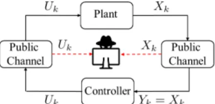
(a) Learning: During this phase, the attacker eavesdrops and learns the system, without altering the input signal to the controller (Yk=Xk).
(b) Hijacking: During this phase, the attacker hijacks the system and intervenes as a MITM in two places: acting as a fake plant for the controller (Yk=Vk) by impersonating the legitimate sensor, and as a malicious controller (U˜k) for the plant aiming to destroy the plant. Fig. 1: System model during learning-based attack phases.
performance for security.
The outline of the rest of the paper is as follows. The notations used in this work are detailed in Sec. I-A. For ease of exposition, we start by presenting the problem for the special case of scalar linear plants in Sec. II, and present our main results for this case in Sec. III. We then extend the model and treatment to vector linear and scalar nonlinear plants in Sec. IV and App. A available online in [52], respectively. We conclude the paper in Sec. V with a discussion of future directions. Due to space constraints, the appendices (and some of the proofs) are available online in [52].
A. Notation
Throughout the paper, we use the following notation. We denote byNthe set of natural numbers, and byR—the set of real numbers. All logarithms, denoted bylog, are base 2. We denote byk·kthe Euclidean norm of a vector, and byk·kop— the operator norm induced by it when applied to a matrix. We denote by †the transpose operation of a matrix. For two real-valued functions g andh, g(x) = O(h(x)) as x→ x0 means lim supx→x0|g(x)/h(x)| < ∞, and g(x) = o(h(x)) as x→ x0 means limx→x0|g(x)/h(x)| = 0. We denote by
xji = (xi,· · ·, xj) the realization of the tuple of random variables Xij = (Xi,· · ·, Xj) for i, j ∈ N, i ≤ j. Random
matrices are represented by boldface capital letters (e.g.A) and their realizations are represented by typewriter boldface letters (e.g.A).ABmeans thatA−B is a positive semidefinite matrix, namelyis the Loewner order of Hermitian matrices.
λmax(A) denotes the largest eigenvalue of the matrix A. We represent the random vector with boldface small letters, and xji = (xi,· · ·,xj) for i, j ∈ N, i ≤ j. Px denotes the
distribution of the random vector x with respect to (w.r.t.) probability measure P, whereas fx denotes its probability
density function (PDF) w.r.t. to the Lebesgue measure, if it has one. An event is said to happen almost surely (a.s.) if it occurs with probability one. For real numbersaandb,ab
means ais much less thanb, in some numerical sense, while for probability distributions P and Q, P Q means P is
absolutely continuous w.r.t. Q. dP/dQ denotes the Radon–
Nikodym derivative ofPw.r.t.Q. The Kullback–Leibler (KL)
divergence between probability distributions PX and PY is defined as D(PXkPY), EPX logdPX dPY , PXPY; ∞, otherwise,
where EPX denotes the expectation w.r.t. probability mea-sure PX. The conditional KL divergence between probability
distributions PY|X and QY|X averaged over PX is defined as D PX|Y QY|X PX , EPX˜ h DPY|X= ˜X QY|X= ˜X i , where (X,X˜) are independent and identically distributed (i.i.d.). The mutual information between random variables
X and Y is defined as I(X;Y) , D(PXYkPXPY). The conditional mutual information between random variables X
and Y given random variable Z is defined as I(X;Y|Z),
EPZ˜
h
I(X;Y|Z = ˜Z)i, where(Z,Z˜) are i.i.d. II. PROBLEMSETUP
We consider the networked control system depicted in Fig. 1, where the plant dynamics are described by a scalar, discrete-time, linear time-invariant (LTI) system
Xk+1=aXk+Uk+Wk, (1) whereXk,a,Uk,Wk are real numbers representing the plant state, open-loop gain of the plant, control input, and plant disturbance, respectively, at time k ∈ N. The controller, at time k, observes Yk and generates a control signal Uk as a function ofYk
1. If the attacker does not tamper sensor reading, at any time k ∈N, we have Yk = Xk. We assume that the initial condition X0 has a known (to all parties) distribution and is independent of the disturbance sequence {Wk}. For analytical purposes, we assume that the process {Wk} has i.i.d. Gaussian samples of zero mean and variance σ2 that is known to all parties. We assume, without loss of generality, that W0 = 0, E[X0] = 0, and take U0 = 0. Moreover, to simplify the notation, letZk,(Xk, Uk)denote the state-and-control input at time kand its trajectory up to time k—by
Z1k ,(X1k, U1k).
The controller is equipped with a detector that tests for anomalies in the observed history Yk
1. When the controller detects an attack, it shuts the system down and prevents the attacker from causing further “damage” to the plant. The controller/detector is aware of the plant dynamics (1) and knows the open-loop gain aof the plant. On the other hand, the attacker knows the plant dynamics (1) as well as the plant state Xk, and control inputUk (or equivalently,Zk) at timek (see Fig. 1). However, it does not know the open-loop gaina. We assume the open-loop gain is fixed in time, but unknown to the attacker (as in the frequentist approach [53]).
Never-theless, it will be convenient, for algorithm aid, to assume a prior over the open-loop gain of the plant, and treat it as a random variableA, that isfixed across time, whose PDFfAis known to the attacker, and whose realizationais known to the controller (cf. Sec. V-D). We assume all random variables to exist on a common probability space with probability measure
P, and Uk to be a measurable function of Y1k for all time
k∈N. We also denote the probability measure conditioned on
A=abyPa. Namely, for any measurable eventC, we define Pa(C) =P(C|A=a).
Ais assumed to be independent ofX0 and{Wk|k∈N}.
A. Learning-based Attacks
We now defineLearning-based attacks that consist of two disjoint, consecutive, passive and active phases (cf. Sec. V-C). Phase 1: Learning.During this phase, the attacker passively observes the control input and the plant state to learn the open-loop gain of the plant. As illustrated in Fig. 1a, for all k ∈ [0, L], the attacker observes the control inputUk and the plant state Xk, and tries to learn the open-loop gain a, where L is the duration of the learning phase. We denote by Aˆ the attacker’s estimate of the open-loop gaina. • Phase 2: Hijacking. In this phase, the attacker aims to destroy the plant viaU˜k while remaining undetected. As illus-trated in Fig. 1b, from timeL+ 1and onward the attacker hi-jacks the system and feeds a malicious control signalU˜kto the plant and a fictitious sensor readingYk=Vkto the controller.• We assume that the attacker can useany arbitrarylearning algorithm to estimate the open-loop gainaduring the learning phase, and when the estimation is completed, we assume that during the hijacking phase the fictitious sensor reading is con-structed, in a model-based manner (cf. Sec. V-B), as follows
Vk+1= ˆAVk+Uk+ ˜Wk, k=L, . . . , T−1, (2) whereW˜k fork=L, . . . , T−1 are i.i.d. GaussianN(0, σ2);
Uk is the control signal generated by the controller, which is fed with the fictitious virtual signalVk by the attacker;VL=
XL; andAˆ is the estimate of the open-loop gain of the plant at the conclusion of Phase 1.
B. Detection
The controller/detector, being aware of the dynamic (1) and the open-loop gain a, attempts to detect possible attacks by testing for statistical deviations from the typical behavior of the system (1). More precisely, under the legitimate system operation (corresponding to thenull hypothesis), the controller observation Yk behaves according to
Yk+1−aYk−Uk(Y1k)∼ i.i.d.N(0, σ 2
). (3) In the case of an attack, during Phase 2 (k > L), (3) can be rewritten as Vk+1−aVk−Uk =Vk+1−aVk+ ˆAVk−AVˆ k−Uk (4a) = ˜Wk+ ˆ A−aVk, (4b) where (4b) follows from (2). Hence, the estimation error( ˆA−
Since the Gaussian PDF with zero mean is fully charac-terized by its variance, we shall follow [29], and test for anomalies in the latter, i.e., test whether the empirical variance of (3) is equal to the second moment of the plant disturbance
EW2. To that end, we shall use a test that sets a confidence
interval of length2δ >0around the expected variance, i.e., it checks whether 1 T T X k=1 Yk+1−aYk−Uk(Y1k) 2 ∈(Var [W]−δ,Var [W] +δ), (5)
whereT is called thetest time. That is, as is implied by (4), the attacker deceives the controller and remains undetected if
1 T L X k=1 Wk2+ T X k=L+1 ( ˜Wk+ ( ˆA−a)Vk)2 ! ∈(Var [W]−δ,Var [W] +δ). C. Performance Measures
Definition 1. The hijack indicator at test timeT is defined as ΘT ,
(
0, ∀j≤T : Yj=Xj; 1, otherwise.
ΘT is an oracle, and at the test timeT the controller usesY1T to construct an estimate ΘˆT of ΘT. More precisely, ΘˆT = 0
if (5) occurs, otherwise ΘˆT = 1. •
Definition 2. The probability of deception is the probability of the attacker deceiving the controller and remaining undetected at the time instant T
PDeca,T ,Pa ˆ ΘT = 0 ΘT = 1 ; (6)
the detection probability at test time T is defined as
PDeta,T ,1−PDeca,T.
Likewise, the probability of false alarm is the probability of detecting the attacker when it is not present, namely
PFAa,T ,Pa ˆ ΘT = 1 ΘT = 0 . •
Applying Chebyshev’s inequality to (5) and noting that the system disturbances are i.i.d. Gaussian of varianceσ2, we have
PFAT ≤ Var[W
2]
δ2T =
3σ4
δ2T.
Further define the deception, detection, and false-alarm prob-abilities w.r.t. the probability measureP, without conditioning
onA, and denote them by PT
Dec,PDetT , andPFAT , respectively. For instance, PDetT is defined, w.r.t. a PDFfA of A, as
PDetT ,PΘˆT = 1 ΘT = 1 = Z ∞ −∞
PDeta,TfA(a)da. (7) III. STATEMENT OF THE RESULTS
In this section, we describe our main results for the case of scalar plants. We provide lower and upper bounds on the deception probability (6) of the learning-based attack (2), where the estimate Aˆ in (2) may be constructed using an
arbitrary learning algorithm. Our results are valid for any measurable control policy Uk. We find a lower bound on the deception probability by characterizing what the attacker can at least achieve using a least-squares (LS) algorithm, and we derive an information-theoretic converse for any learning algorithm using Fano’s inequality [54, Chs. 2.10 & 7.9]. While our analysis is restricted to the asymptotic case,T → ∞, it is straightforward to extend it to the non-asymptotic case.
For analytical purposes, we assume that the power of the fictitious sensor reading is equal to β−1<∞, namely
lim T→∞ 1 T T X k=L+1 Vk2= 1/β a.s. w.r.t. Pa. (8) Remark1.Assuming the control policy is memoryless, namely
Uk is only dependent on Yk, the process Vk is Markov for
k ≥ L+ 1. By further assuming that L = o(T) and using the generalization of the law of large numbers for Markov processes [55], we deduce lim T→∞ 1 T T X k=L+1 Vk2≥Var [W] a.s. w.r.t.Pa. Hence, in this case, we haveβ ≤1/Var [W]. Also, when the control policy is linear and stabilizes (2), that isUk=−ΩYk and |Aˆ−Ω| <1, it is easy to verify that (8) holds true for
β= (1−( ˆA−Ω)2)/Var [W]. The assumption in (8) can also be relaxed as described in Remarks 4 and 6, in the sequel. • In the following lemma we show that for any learning-based attack (2), as T → ∞ the empirical variance used in the variance test (5) can be expressed in terms of the estimation error. The result follows from the strong law of large numbers applied to martingale difference sequences [56, Lem. 2, part iii]; it is proved in App. C-A [52].
Lemma 1. Consider any learning-based attack (2) and any measurable control policy{Uk}such that the fictitious sensor reading power satisfies(8). Then, the variance test(5)reduces a.s., w.r.t.Pa, to lim T→∞ 1 T T X k=1 [Yk+1−aYk−Uk(Y1k)]2= Var [W] + ( ˆA−a)2 β .
A. Lower Bound on the Deception Probability
To provide a lower bound on the deception probabilityPDeca,T, we consider a specific estimateAˆat the conclusion of the first phase by the attacker. Namely, we use LS estimation due to its efficiency and amenability to recursive update over observed incremental data [44]–[46]. The LS algorithm approximates the overdetermined system of equations
X2 X3 .. . XL =A X1 X2 .. . XL−1 + U1 U2 .. . UL−1 ,
by minimizing the Euclidean distance Aˆ = argminA kXk+1−AXk−Ukkto estimate (or “identify”) the plant, the solution to which is
ˆ A= PL−1 k=1(Xk+1−Uk)Xk PL−1 k=1 X 2 k a.s. w.r.t.Pa. (9) Remark 2. (9) is well-defined sincePa(Xk = 0) = 0, as we assumed Wk are i.i.d. zero-mean Gaussian for allk∈N. •
We now lower bound the deception probability of an attacker that utilizes LS estimation (9) under the variance test and in the presence of any measurable control policy for which (8) holds. The following theorem demonstrates the existence of a learning-based attack that satisfies this lower bound. As other learning algorithms may lead to better estimates, this also serves as a lower bound on the attacker’s deception probability in the general case.
Theorem 1. Consider LS (9) learning-based attack (2) and any measurable control policy {Uk} such that the fictitious sensor readings satisfy (8). Then, the asymptotic deception probability under the variance test (5)is lower bounded as
lim T→∞P a,T Dec=Pa |Aˆ−a|<pδβ (10a) ≥Pa PL−1 k=1WkXk PL−1 k=1Xk2 <pδβ (10b) ≥1− 2 (1 +δβ)L/2. (10c)
Proof: (10a) follows from Lem. 1, and the dominated convergence theorem [55]. For details see App. C-B [52]. Clearly, the estimation error of the LS algorithm (9) is [44]
ˆ A−a= PL−1 k=1WkXk PL−1 k=1X 2 k a.s. w.r.t. Pa. (11) Consequently, by (10a), a learning-based attack (2) can at least achieve the asymptotic deception probability (10b). Finally, (10c) holds by the concentration of measure [44, Th. 4] by noting that Uk is a measurable function of Y1k = X1k, for
k∈ {1, . . . , L}.
Remark 3. We can study the special case of Theorem 1 for a linear controller. Using the value ofβ calculated in Remark 1 for a linear controllerUk =−ΩYkwhen|Aˆ−Ω|<1, we can rewrite (10c) as lim T→∞P a,T Dec ≥1− 2 1 +δ1−( ˆVar[A−Ω)W]2 L/2. (12) In this case, for a fixed L, as Var [W] increases the lower bound in (12) decreases. The reduction of the attacker’s suc-cess rate can be explained by noticing that LS estimation (9) is based on minimizingkXk+1−AXk−Ukk, and the precision of this estimate decreases as Var [W] increases. • Remark 4. By replacing the limit with limsup in the lower bound in Thm. 1, the result holds even if the limit in (8) does not exist. Also, if the limit in (8) is infinite then either the attacker or the controller are doing a poor job, as described next. Assume the attacker uses an estimate Aˆ such that at the conclusion of the learning phaseAˆbelongs to the interval (A−δ0, A+δ0), for a small value of δ0 >0. In this case, if
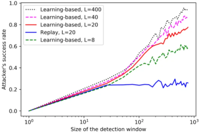
Fig. 2: The attacker’s success ratePDeca,T versus the size of the detection windowT.
the power of the fictitious sensor reading tends to infinity, then the controller is not robust. On the other hand, assume that the controller stabilizes the system with any open-loop gain that belongs to the interval(A−δ0, A+δ0), whereδ0 >0. In this case, if the power of fictitious sensor tends to infinity, then the attacker’s estimate at the conclusion of the learning phase, does not belong to the interval(A−δ0, A+δ0), i.e. the absolute value of the attacker’s estimation error is larger thanδ0. Example 1. In this example, we compare the empirical performance of the variance-test with our developed bound in Thm. 1. At every timeT, the controller tests the empirical variance for anomalies over a detection window [1, T], using a confidence interval2δ >0around the expected variance (5). Here,a= 1,δ= 0.1,Uk =−0.88aYk for all1≤k≤T = 800, and {Wk} are i.i.d. Gaussian N(0,1), and 500 Monte Carlo simulations were performed.
The learning-based attacker (2) uses the LS algorithm (9) to estimate aand, as illustrated in Fig. 2, the attacker’s success rate increases as the duration of the learning phaseLincreases. This is in agreement with (10c) since the attacker can improve its estimate of a and the estimation error |Aˆ−a| reduces as L increases. As discussed in Sec. II-C, the false alarm rate decays to zero as the size of the detection window T
tends to infinity. Hence, for a sufficiently large detection window, the attacker’s success rate could potentially tend to one. Indeed, such behavior is observed in Fig. 2 for a learning-based attacker (2) withL= 400. Fig. 2 also illustrates that our learning-based attack outperforms the replay attack. A replay attack with a recording length ofL= 20and a learning-based attack with a learning phase of lengthL= 20are compared, and the success rate of the replay attack saturates at a lower value. Moreover, a learning-based attack with a learning phase of lengthL= 8has a higher success rate than a replay attack with a larger recording length ofL= 20. •
B. Upper Bound on the Deception Probability
We now derive an upper bound on the deception proba-bility (6) of any learning-based attack (2) where Aˆ in (2) is constructed using any arbitrary learning algorithm, for
any measurable control policy, when A is distributed over a symmetric interval [−R, R]. Since the uniform distribution has the highest entropy among all distributions with finite support [54, Ch. 12], we assume that A has a uniform prior over the interval[−R, R]. We further assume that the attacker knows this distribution (including the value ofR), whereas the controller knows the true realization of A(as before). Theorem 2. For any R > 0, let A be distributed uniformly over [−R, R], and consider any measurable control policy {Uk}and any learning-based attack(2)such that the fictitious sensor readings satisfy (8) with√δβ≤R. Then, the asymp-totic deception probability, when using the variance test (5), is upper bounded as lim T→∞P T Dec=P(|A−Aˆ|< p δβ) (13a) ≤Λ,I(A;Z L 1) + 1 log(R/√δβ) . (13b) In addition, if for allk∈ {1, . . . , L},A→(Xk, Z1k−1)→Uk is a Markov chain, then for any sequence of probability measures {QXk|Z1k−1}, such that for all
k ∈ {1, . . . , L} PXk|Zk1−1 QXk|Zk1−1, we have Λ≤ PL k=1D PXk|Zk1−1,A QXk|Z1k−1 PZk1−1,A + 1 log R/√δβ .(14)
Proof: (13a) follows from (7), (10a), and Tonelli’s theo-rem [55]. For details see App. D [52]. (13b) follows by noting that since the attacker observes the plant state and control input during the learning phase which lastsLsteps, and since
A → (X1L, U1L)→Aˆ constitutes a Markov chain, using the continuous domain version of Fano’s inequality [57, Prop. 2], we have inf ˆ A P ˆ A−A ≥ p δβ≥1−I(A;Z L 1) + 1 log(R/√δβ), whenever √δβ≤R. Finally, (14) follows the arguments of [58] and is proven, for completeness, in App. D-B [52]. Remark5. By looking at the numerator in (13b), it follows that the bound on the deception probability becomes looser as the amount of information revealed about the open-loop gainAby the observation ZL
1 increases. On the other hand, by looking at the denominator, the bound becomes tighter asRincreases. This is consistent with the observation of Zames [58] that system identification becomes harder as the uncertainty about the open-loop gain of the plant increases. In our case, a larger uncertainty interval R corresponds to a poorer estimation of
A by the attacker, which leads, in turn, to a decrease in the achievable deception probability. The denominator can also be interpreted as the intrinsic uncertainty ofAwhen it is observed at resolution √δβ, as it corresponds to the entropy of the random variableA when it is quantized at such resolution. • In conclusion, Thm. 2 provides two upper bounds on the deception probability. The first bound (13b) clearly shows that increasing the privacy of the open-loop gain A—manifested in the mutual information between A and the state-and-control trajectory ZL
1 during the exploration phase—reduces
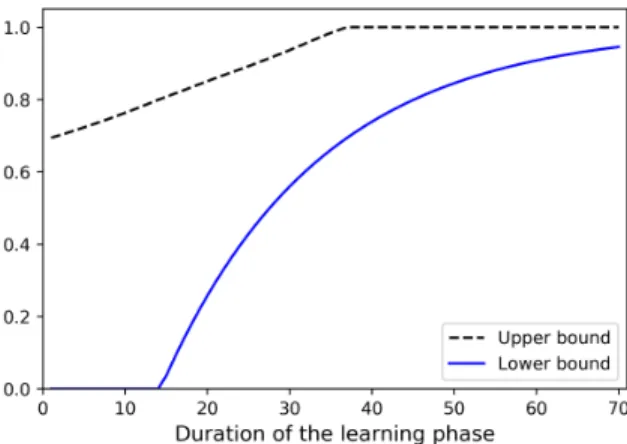
Fig. 3: Comparison of the lower and upper bounds on the deception probability, of Thm. 1 and Corol. 1, respectively.
the deception probability. The second bound (14) allows free-dom in choosing the auxiliary probability measureQXk|Zk1−1,
making it a rather useful bound. For instance, by choosing
QXk|Zk1−1 ∼ N(0, σ
2), for allk∈
N, we can rewrite the upper
bound (14) in term ofEP
(AXk−1+Uk−1)2as follows. The proof of the following corollary can be found in [52]. Corollary 1. Under the assumptions of Thm. 2, if for allk∈ {1, . . . , L},A→(Xk, Z1k−1)→Uk is a Markov chain, then the asymptotic deception probability upper bounded as
lim T→∞P T Dec≤G(Z L 1), (15a) G(Z1L), loge 2σ2 PL k=1EP (AXk−1+Uk−1)2+ 1 log R/√δβ .(15b)
Remark6. Following the same discussion as in Remark 4, by replacing the limit with liminf in the upper bound in Thm. 2, the derived results remain true even if (8) does not happen.• The next example compares the lower and upper bounds on the deception probability of Thm. 1 and Corol. 1.
Example 2. Thm. 1 provides a lower bound on the deception probability given A = a. Hence, by applying the law of total probability w.r.t. the PDF fA as in (7), we can apply the result of Thm. 1 to provide a lower bound also on the average deception probability for a random open-loop gainA. In this context, Fig. 3 compares the lower and upper bounds on the deception probability provided by Thm. 1 and Corol. 1, augmented with the trivial cases of zero and one probability, namely max{0,1−(2/(1 +δβ)L/2)}, and min{1, G(ZL
1)}, where A is distributed uniformly over [−0.9,0.9]. Equation (15a) is valid when the control input is not a function of random variableA; hence, we assumedUk =−0.045Ykfor all timek∈N. Hereδ= 0.1,{Wk}are i.i.d. Gaussian with zero mean and variance of0.16, and for simplicity, we assume the limit in (8) exists [cf. Remarks 4 and 6], and we letβ= 1.1. Although in general the attacker’s estimation of the random open-loop gain A and consequently the power of fictitious sensor reading (8) vary based on the learning algorithm and the realization of A, the comparison of the lower and upper bounds in Fig. 3 is restricted to a fixedβ. 2000Monte Carlo
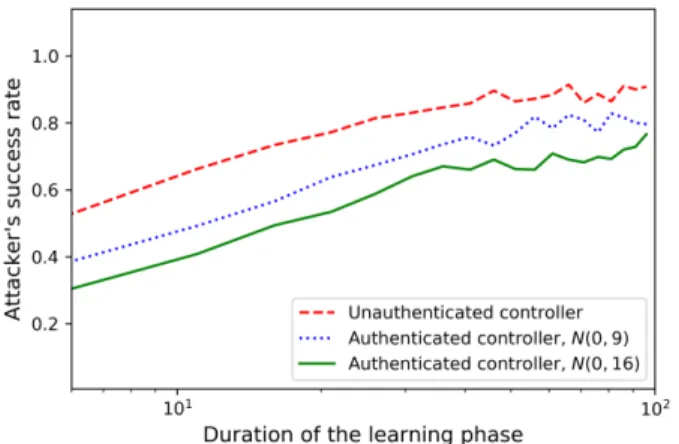
Fig. 4: The attacker’s success ratePDeca,T versus the duration of the learning phaseL.
simulations were performed.
Fig. 3 also illustrates the gap between these lower and upper bounds on the deception probability. By restricting the class of control policies or learning algorithms one might be able to derive tighter results at the cost of losing generality. •
C. Privacy-enhancing Signal
For a given duration of the learning phaseL, to increase the security of the system, at any time k the controller can add a privacy-enhancing signal Γk to an unauthenticated control policy {U¯k|k∈N}:
Uk = ¯Uk+ Γk, k∈N. (16)
We refer to such a control policy Uk as the authenticated control policy U¯k. We denote the states of the system that would be generated if only the unauthenticated control sig-nal U¯k
1 were applied by X¯1k, and the resulting trajectory—by
¯
Z1k,( ¯X1k,U¯1k).
The following numerical example illustrates the effect of the privacy-enhancing signal on the deception probability. Example 3. Here, the attacker uses the LS algorithm (9), the detector uses the variance test (5), a = 1, T = 600, δ = 0.1, and{Wk} are i.i.d. standard Gaussian. We compare the attacker’s success rate, the empirical PDeca,T, as a function of the durationLof the learning phase for three different control policies: I) unauthenticated control signal U¯k
1 = −aYk for allk, II) authenticated control signal (16), whereΓk are i.i.d. GaussianN(0,9), III) authenticated control signal (16), where Γk are i.i.d. Gaussian N(0,16). As illustrated in Fig. 4, for both the authenticated and unauthenticated control signals, the attacker’s success rate increases as the duration of the learning phase increases. This is in agreement with (10c) since the attacker can improve its estimate ofaasLincreases. Further, for a fixedLthe attacker performance deteriorates as the power of privacy-enhancing signalΓkincreases. Namely,Γkhampers the learning process of the attacker and the estimation error |Aˆ−a|increases as the power of the privacy-enhancing signal increases. 500 Monte Carlo simulations were performed. • Remark7. A “good” privacy-enhancing signal entails little in-crease in the control cost [59] compared to its unauthenticated
version while providing enhanced detection probability (6) and/or false alarm probability. Finding the optimal privacy-enhancing signal is left for future research. We remark that since the submission of this paper [1], [52], some latter literature has appeared that builds on it. In particular, in a follow-up work [60], Ziemann and Sandberg focused on designing optimal privacy-enhancing signal, by studying the optimal control problem of linear systems regularized with Fisher information, where the latter serves as a proxy to the estimation quality ofAvia the Cramer–Rao lower bound. • One may envisage that superimposing any noisy signalΓk on top of the control policy {U¯k|k ∈ N} would necessarily
enhance the detectability of any learning-based attack (2) since the observations of the attacker are in this case noisier. However, it turns out that injecting a strong noise for some learning algorithm may, in fact, speed up the learning process as it improves the power of the signal magnified by the open-loop gains with respect to the observed noise [44]. Any signalΓk that satisfies the condition proposed in the following corollary, whose proof available in [52], will provide enhanced guarantees on the detection probability when the attacker uses any arbitrary learning algorithm to estimate the uniformly distributedAover the symmetric interval [−R, R].
Corollary 2. For any control policy {U¯k|k ∈ N} with
tra-jectory Z¯1k = ( ¯X1k,U¯1k) and its corresponding authenticated control policyU1k (16)with trajectoryZ1k= (X1k, U1k), under the assumptions of Corollary 1, if for all k∈ {1, . . . , L−1}
EP
Ψ2k+ 2Ψk(AX¯k+ ¯Uk)
<0, (17) where Ψk , Pkj=1Ak−jΓj, for any L ≥ 2, the following majorization ofG(15b) holds:
G(Z1L)< G( ¯Z1L). (18) Remark 8. Corol. 2 can be generalized by replacing the limit with liminf in (8) [cf. Remarks 4 and 6]. •
Example 4. In this example, we describe a class of privacy-enhancing signals that yield better guarantees on the decep-tion probability. For all k ∈ {2, . . . , L}, clearly, Ψk−1 =
−(AX¯k−1+ ¯Uk−1)/η satisfies the condition in (17) for any
η ≥ 3. Thus, by choosing the privacy-enhancing signals Γ1 = −(AX¯1 + ¯U1)/η, and Γk = −(AX¯k + ¯Uk)/η −
Pk−1
j=1A k−1−jΓ
j for all k ∈ {3, . . . , L}, (18) holds. A numerical example for this authentication policy demonstrates a decrease in the deception probability at the expense of a higher control cost, and it can be found in App. B-A [52]. • Remark 9. The privacy-enhancing signal introduced in this work is related to the dynamic watermarking signal [26], [29], [30], which are unique signatures that are availableonlyto the controller. In contrast, in our setup (depicted in Fig. 1b), the attacker has access to the signal generated by the controller. Thus, by reading the control input at timekand constructing the ficticous sensor reading Vk+1, as in (2), the attacker can construct a fictitious sensor reading containing any watermark signal inscribed by the controller. It follows that techniques based on dynamic watermarking that rely on the privacy of
such signal break down in the case where attacks have access to the control signal generated by the controller. Instead, we take advantage of the authentication signal in a different way: since the attacker does not have full knowledge about the system dynamics, this signal is used to hamper the learning process of the attacker during the learning phase. •
IV. EXTENSION TOVECTORSYSTEMS
We now generalize our results to vector systems. Consider the networked control system depicted in Fig. 1, with the plant dynamics replaced by a vector plant:
xk+1=Axk+uk+wk, (19) where xk ∈ Rn×1, uk ∈ Rn×1, A ∈ Rn×n, wk ∈ Rn×1
represent the plant state, control input, open-loop gain of the plant, and plant disturbance, respectively, at time k∈N. The controller, at timek, observesykand generates a control signal uk as a function of yk1, and yk = xk at times k ∈ N at
which the attacker does not tamper the sensor reading. We assume that the initial conditionx0has a known (to all parties) distribution and is independent of the disturbance sequence {wk}. For analytical purposes, we further assume {wk} is a process with i.i.d. multivariate Gaussian samples of zero mean and a covariance matrixΣthat is known to all parties. Without loss of generality, we assume that w0 = 0, E[x0] = 0, and
takeu0= 0.
We assume the attacker uses the vector analogue of learning based attacks described in Sec. II-A where the attacker can use anylearning algorithm to estimate the open-loop gain matrix
Aduring the learning phase. The estimationAˆ constructed by the attacker at the conclusion of the learning phase is utilized to construct the fictitious sensor readings {vk} according to the vector analogue of (2), where {w˜k|k = L, . . . , T −1} are i.i.d. multivariate Gaussian with zero mean and covariance matrix Σ.
Similar to the scalar case, for analytical purposes, we assume that the power of the fictitious sensor reading is equal to1/β <∞ [cf. Remarks 1 and 4], namely
lim T→∞ 1 T T X k=L+1 kvkk2= 1 β a.s. w.r.t. PA. (20)
Since the zero-mean multivariate Gaussian distribution is completely characterized by its covariance matrix, we shall follow [29] and test for anomalies in the latter. To that end, define the error matrix
∆,Σ− 1 T T X k=1 yk+1−Ayk−uk yk+1−Ayk−uk † .
As in (5), we use a test that sets a confidence interval, with respect to the norm, around the expected covariance matrix, i.e., it checks whether
k∆kop≤γ, (21)
at the test timeT. For the sake of analysis, we use the operator norm in (21), which satisfies the sub-multiplicativity property.
The following lemma provides a necessary and sufficient condition for any learning-based attack [the vector analogue of (2)] to deceive the controller and remain undetected, for a multivariate plant (19) under a covariance test (21), in the limit ofT → ∞; its proof is available in [52].
Lemma 2. Consider the multivariate plant (19), and any learning-based attack analogous to (2), with fictitious sensor reading power that satisfies(20), and any measurable control policy{uk}. Then, the attacker can deceive the controller and remain undetected, under the covariance test (21), a.s. in the limit T → ∞, if and only if
lim T→∞ 1 T T X k=L+1 ( ˆA−A)vkv†k( ˆA−A) † op ≤γ. (22) Lem. 2 has the following important implication.
lim T→∞ 1 T T X k=L+1 ( ˆA−A)vkv†k( ˆA−A) † op (23a) ≤ lim T→∞ 1 T T X k=L+1 ( ˆA−A)vk(( ˆA−A)vk) † op(23b) ≤ lim T→∞ 1 T T X k=L+1 ( ˆA−A)vk 2 op (23c) ≤ ˆ A−A 2 op /β , (23d)
where (23b) follows from the triangle inequality, (23c) and (23d) follow from the sub-multiplicativity of the operator, the identity kvkk = kvkkop and by putting the power constraint (20) into force.
If kAˆ −Ak2
op ≤ γβ, (22) holds in the limit of T → ∞, then the attacker is able to deceive the controller and remain undetected a.s., by Lem. 2. Equation (23) then implies that the norm of the estimation error,kAˆ−Akop, dictates the ease with which an attack can go undetected. This is used next to develop a lower bound on the deception probability.
A. Lower Bound on the Deception Probability
We start by observing that in the case of multivariate systems, and in contrast to their scalar counterparts, some control actions might not reveal the entire plant dynamics, and in this case the attacker might not be able to learn the plant completely. This phenomenon is captured by the persistent excitation property of control inputs, which describes control-action signals that are sufficiently rich to excite all the system modes that will allow to learn them. While avoiding persis-tently exciting control inputs can be used as a way tosecure the system against learning-based attacks, here, we assume a probabilistic variant of this property [58], [61].
Definition 3 (Persistent excitation). Given a plant (19), ζ >
0, and ρ ∈ [0,1], the control policy uk is (ζ, ρ)-persistently exciting if there exists a timeL0∈Nsuch that, for allτ≥L0,
PA
1
τGτ ζIn×n
whereGτ is the sum of the state Gramians up to timeτ: Gτ, τ X k=1 xkx†k. (25) As in Sec. III-A, to find a lower bound on the deception probability PDecA,T, we consider a specific estimate of A, ob-tained via the LS estimation algorithm, analogous to (9), at the conclusion of the first phase by the attacker:
ˆ A= 0n×n, det(GL−1) = 0; L−1 P k=1 (xk+1−uk)x†kG −1 L−1, otherwise, (26)
where0k×` denotes an all zero matrix of dimensionsk×`. Next, we show an upper bound on the estimation-error norm, kAˆ −Akop, of the above LS algorithm (26), and use it to extend the bound in (10) to the vector case. A complete proof is available in [52].
Lemma 3. Consider the vector plant (19). If the attacker constructsAˆ using LS estimation(26), and the controller uses a policy{uk}for which the event in(24)occurs forτ =L−1, that is GL−1/(L−1)ζIn×n. Then, we have
kAˆ −Akop≤ 1 ζL L−1 X k=1 kwkx†kkop a.s. w.r.t. PA. (27) The following theorem provides a lower bound on the deception probability of an attacker that utilizes LS estima-tion (26), and its proof can be found in [52]. As discussed before Thm. 1, since the attacker might be able to construct better estimates using other learning algorithms, this also serves as a lower bound on the attacker’s deception probability in the general case.
Theorem 3. Consider the plant(19)with a(ζ, ρ)-persistently exciting control policy {Uk} from time L0, and LS (26) learning-based attack [the vector analogue of (2)] such that the fictitious sensor reading power satisfies (20) and with a learning phase of durationL≥L0+ 1. Then, the asymptotic deception probability, when using the covariance test (21), is bounded from below as
lim T→∞P A,T Dec≥PA kAˆ−Akop< p γβ (28a) ≥ρPA 1 ζL L−1 X k=1 kwkx†kkop< p γβ ! . (28b) Remark 10. The bound (10c) for scalar systems, which is independent of the control policy and state value, has been developed using the concentration bounds of [44] for the scalar LS algorithm (9). To the best of our knowledge, there are no similar concentration bounds for the vector variant of the LS algorithm (9) which work for any A, and a large class of control policies. Looking for such bounds, which are independent of the state value, seems an interesting research venue. The lower bound (28b) is similar to (10b), while (10b) is stronger for the particular case of scalar system, as the upper bound on the estimation error derived in Lem. 3 is not required for the scalar case, and the estimation error is given in (11).•
Fig. 5: The attacker’s success ratePDecA,T versus the size of the detection windowT.
Example 5. In this example, we compare the empirical performance of the covariance test against the learning-based attack which utilizes LS estimation (26), and the replay attack. At every time k, the controller tests the empirical covariance for anomalies over a detection window[1, T], using a confidence interval 2γ > 0 around the operator norm of error matrix ∆ (21). Since we are considering the Euclidean norm for vectors, the induced operator norm amounts to k∆kop = p λmax(∆†∆). Here, γ = 0.1, uk = −0.9Ayk for all1≤k≤T = 600, A= 1 2 3 4 , Σ= 1 0 0 2 . (29) Fig. 5 presents the performance averaged over180runs of a Monte Carlo simulation. It illustrates that the vector variant of our learning-based attack alsooutperformsthe replay attack. A learning-based attack with a learning phase of lengthL= 40 has a higher success rate than a replay attack with a larger recording length of L = 50. Similarly to the discussion for scalar systems in Sec. II-C, the false-alarm rate decays to zero as the size of the detection windowT tends to infinity. Thus, the success rate of learning-based attacks increases as the size of the detection window increases. Finally, as illustrated in Fig. 5, the attacker’s success rate increases as the duration of the learning phaseLincreases, since the attacker improves
its estimate ofAas Lincreases. •
An example that investigates the effect of privacy-enhancing signals on the empirical deception probability of the learning-based attacks on the vector systems is in App. B-B [52].
V. DISCUSSION ANDFUTUREWORK A. Upper Bound on the Deception Probability
The upper bound in (23), which relates the deception criterion (22) to the estimation errorkAˆ−Akop, is used to find the lower bound (28). Finding a corresponding lower bound in term ofkAˆ−Akop for (23a) is the first step in extending our results in Thm. 2 to vector systems. Finding an upper bound on the deception probability for vector linear and scalar nonlinear systems, where the attacker can useanylearning algorithm, is left open for future work.
B. Model-based vs. Model-free
In this work, we mainly concentrated on linear systems; we assumed the attacker constructs the fictitious sensor reading, in a model-based manner, according to the linear model (2) and its vector variants. In general, as discussed in App. A available online in [52], the system can be nonlinear, and the attacker might not be aware of the linearity or non-linearity of the dynamics. Comparing the deception probability for the vast range of model-free and model-based learning methods [41], [45], [62] is an interesting research venue.
C. Continuous Learning and Hijacking
In this work, we assumed two disjoint consecutive phases (recall Sec. II-A): learning and hijacking, which are akin to the exploration and exploitation phases of reinforcement learning (RL) [63]. Indeed, in this two-phase process, the attacker explores the system until it reaches a desired deception probability and then moves to the exploitation phase during which it drives the system to instability as quickly as it can. The two phases are completely separate due to the inherent tension between them: exploiting the system without properly exploring it during the learning (silent) phase increases the chances of being detected.
Despite the naturalness of two-phase attacks, just like in RL [63], one may consider more general strategies where exploration and exploitation are intertwined and gradual: as time elapses, the attacker can gain better estimates of the observed system and gradually increase its detection-limited attack. In these terms, our two-phase attack can be regarded as a two-stage approximation of the gradual attack and provides achievability bounds for such attacks. Studying more general attacks is a research venue that is left for future study.
D. Oblivious Controller
A more realistic scenario is the one in which neither the attacker nor the controller are aware of the open-loop gain of the plant. In this scenario, both parties strive to learn the open-loop gain—posing two conflicting objectives to the controller, who, on the one hand, wishes to speed up its own learning process, while, on the other hand, wants to slow down the learning process of the attacker.
In such a situation, standard adaptive control methods are clearly insufficient, as no asymmetry between the attacker and the controller can be achieved under the setting of Sec. II. To create a security leverage over the attacker, the controller needs to utilize a judicious privacy-enhancing signal: A properly de-signed privacy-enhancing signal should enjoy a positive double effect by facilitating the learning process of the controller while hindering that of the attacker at the same time. Note that, in such a scenario, while the controller knows both U¯k andΓk, the attacker is cognizant of only their sum (16)—Uk. This is reminiscent of strategic information transfer [64].
Finally, we note that, unless the controller is able to detect an MITM attack (the attacker’s hijacking phase), its learning process will be hampered by the fictitious signal that is generated according to the virtual system of the attacker (2).
E. Moving Target Defense
In our setup the attacker has full access to the control signal (see Fig. 1), and at timek+1the attacker uses the control input
Uk to construct the fictitious sensor readingVk+1 according to (2). Thus, thewatermarkingsignal [26], the private random signature, might not be an effective way to counter the learning based attacks [cf. Remark 9]. Here, we introduced the privacy-enhancing signal (16) to impede the learning process of the attacker and decrease the deception probability. Another technique that has been developed in the literature to counter attacks, where the attacker has full system knowledge, is having the controller covertly introduce virtual state variables unknown to the attacker but that are correlated with the ordinary state variables, so that modification of the original states will impact the extraneous states. These extraneous states can act as amoving target[35]–[38] for the attacker. A similar technique is the so-calledbaiting, which adds an offset to the system dynamic [39], [40]. In practice, this technique breaks the information symmetry between the attacker—which has the full system knowledge, and the controller. Using such defense techniques to hamper the learning process of our proposed attacker, is an interesting research venue. In this context, the controller, by potentially sacrificing the optimally of the control task, can act in an adversarial learning setting. Assuming that the control can covertly introduce a virtual part to the dynamics, for any given duration of the learning phase
L (see Fig. 1), sufficiently fast changes in the cipher part of the dynamic can drastically hamper the learning process of the attacker. Also, as discussed in App. A [52], adding a rich nonlinearity to the dynamics can be used as a way to secure the system against learning-based attacks.
F. Optimal testing
Throughout this work, we have assumed that the controller tests the integrity of the system at a specific time step T, that tends to infinity. Since the controller does not know the exact time instant at which an attack might occur, a more realistic scenario would be that of continuous testing, i.e., that in which the integrity of the system is tested at every time step and where the false alarm and deception probabilities are defined with a union over time. We leave this treatment for future research.
In addition, following [29], we have considered the variance-based test, which searches for anomalies in the empirical variance, i.e., whether it falls outside a confidence interval of length 2δ [cf. (5)]. Studying the optimal detector for learning-based attacks is an interesting research venue. G. Further Future Directions
Other future directions can explore the extension of the established results to partially-observable linear vector systems where the input (actuation) gain is unknown, characterising securable and unsecurable subspaces [65] for learning-based attacks, revising the attacker full access to both sensor and control signals, designing optimal privacy-enhancing signals (recall Remark 7) for linear and nonlinear systems, investigat-ing the scenario in which the attacker is oblivious of the noise
covariance matrix or more generally the noise statistics, and studying the relation between our proposedprivacy-enhancing signal with the noise signal utilized to achieve differential privacy [66]. Finally note that we assume that the attacker does not know the control strategy applied by the controller but is privy to the control actions generated by the controller. In the case where the attacker knows the control policy (or control objectives), it can do a much better job in learning the system dynamics, which is an interesting research venue.
REFERENCES
[1] M. J. Khojasteh, A. Khina, M. Franceschetti, and T. Javidi, “Authenti-cation of cyber-physical systems under learning-based attacks,” IFAC-PapersOnLine, vol. 52, no. 20, pp. 369–374, 2019.
[2] B. Kehoe, S. Patil, P. Abbeel, and K. Goldberg, “A survey of research on cloud robotics and automation,”IEEE Tran. on auto. sci. and eng., vol. 12, no. 2, pp. 398–409, 2015.
[3] D. I. Urbina, J. A. Giraldo, A. A. Cardenas, N. O. Tippenhauer, J. Valente, M. Faisal, J. Ruths, R. Candell, and H. Sandberg, “Lim-iting the impact of stealthy attacks on industrial control systems,” in Proceedings of the 2016 ACM SIGSAC Conference on Computer and Communications Security, 2016, pp. 1092–1105.
[4] S. M. Dibaji, M. Pirani, D. B. Flamholz, A. M. Annaswamy, K. H. Johansson, and A. Chakrabortty, “A systems and control perspective of CPS security,”Ann. Rev. in Cont., 2019.
[5] M. Jamei, E. Stewart, S. Peisert, A. Scaglione, C. McParland, C. Roberts, and A. McEachern, “Micro synchrophasor-based intrusion detection in automated distribution systems: Toward critical infrastructure security,” IEEE Int. Comp., vol. 20, no. 5, pp. 18–27, 2016.
[6] H. Sandberg, S. Amin, and K. H. Johansson, “Cyberphysical security in networked control systems: An introduction to the issue,”IEEE Cont. Magazine, vol. 35, no. 1, pp. 20–23, 2015.
[7] C.-Z. Bai, F. Pasqualetti, and V. Gupta, “Data-injection attacks in stochastic control systems: Detectability and performance tradeoffs,” Automatica, vol. 82, pp. 251–260, 2017.
[8] V. Dolk, P. Tesi, C. De Persis, and W. Heemels, “Event-triggered control systems under denial-of-service attacks,”IEEE Trans. Cont. Network Sys., vol. 4, no. 1, pp. 93–105, 2017.
[9] Y. Shoukry, M. Chong, M. Wakaiki, P. Nuzzo, A. Sangiovanni-Vincentelli, S. A. Seshia, J. P. Hespanha, and P. Tabuada, “SMT-based observer design for cyber-physical systems under sensor attacks,”ACM Trans. on CPS, vol. 2, no. 1, p. 5, 2018.
[10] Y. Chen, S. Kar, and J. M. Moura, “Cyber-physical attacks with control objectives,”IEEE Trans. Auto. Control, vol. 63, no. 5, pp. 1418–1425, 2018.
[11] D. Shi, Z. Guo, K. H. Johansson, and L. Shi, “Causality countermeasures for anomaly detection in cyber-physical systems,” IEEE Trans. Auto. Control, vol. 63, no. 2, pp. 386–401, 2018.
[12] S. Dibaji, M. Pirani, A. Annaswamy, K. H. Johansson, and A. Chakrabortty, “Secure control of wide-area power systems: Confi-dentiality and integrity threats,” inProc. IEEE Conf. Decision and Cont. (CDC), Miami Beach, FL, USA, 2018, pp. 7269–7274.
[13] R. Tunga, C. Murguia, and J. Ruths, “Tuning windowed chi-squared detectors for sensor attacks,” inAmerican Control Conf. (ACC), Mil-waukee, WI, USA, 2018, pp. 1752–1757.
[14] L. Niu, J. Fu, and A. Clark, “Minimum violation control synthesis on cyber-physical systems under attacks,” inProc. IEEE Conf. Decision and Cont. (CDC), Miami Beach, FL, USA, pp. 262–269.
[15] M. S. Chong, H. Sandberg, and A. M. Teixeira, “A tutorial introduction to security and privacy for cyber-physical systems,” in2019 Europ. Cont. Conf. (ECC), pp. 968–978.
[16] I. Tomi´c, M. J. Breza, G. Jackson, L. Bhatia, and J. A. McCann, “Design and evaluation of jamming resilient cyber-physical systems,” inIEEE Inter. Conf. on Internet of Things (iThings) and IEEE Gr. Comput. and Commu. (GreenCom) and IEEE Cyber. Phy. and So. Comp. (CPSCom) and IEEE Sm. Data (SmartData), 2018, pp. 687–694.
[17] K. Ding, X. Ren, D. E. Quevedo, S. Dey, and L. Shi, “DOS attacks on remote state estimation with asymmetric information,”IEEE Tran. Cont. Net. Sys., vol. 6, no. 2, pp. 653–666, 2018.
[18] A. Teixeira, I. Shames, H. Sandberg, and K. H. Johansson, “A se-cure control framework for resource-limited adversaries,”Automatica, vol. 51, pp. 135–148, 2015.
[19] M. Xue, S. Roy, Y. Wan, and S. K. Das, “Security and vulnerability of cyber-physical,” Handbook on securing cyber-physical critical infras-tructure, p. 5, 2012.
[20] A. Cetinkaya, H. Ishii, and T. Hayakawa, “Networked control under random and malicious packet losses,”IEEE Trans. Auto. Control, vol. 62, no. 5, pp. 2434–2449, 2017.
[21] P. N. Brown, H. P. Borowski, and J. R. Marden, “Security against im-personation attacks in distributed systems,”IEEE Trans. Cont. Network Sys., vol. 6, no. 1, pp. 440–450, 2018.
[22] Y. W. Law, T. Alpcan, and M. Palaniswami, “Security games for risk minimization in automatic generation control,”IEEE Trans. Power Sys., vol. 30, no. 1, pp. 223–232, 2014.
[23] I. Shames, F. Farokhi, and T. H. Summers, “Security analysis of cyber-physical systems usingH2norm,”IET Cont. The. App., vol. 11, no. 11, pp. 1749–1755, 2017.
[24] N. Hashemi, C. Murguia, and J. Ruths, “A comparison of stealthy sensor attacks on control systems,” inAmerican Control Conf. (ACC). IEEE, 2018, pp. 973–979.
[25] R. S. Smith, “A decoupled feedback structure for covertly appropriating networked control systems,”IFAC Proceedings Volumes, vol. 44, no. 1, pp. 90–95, 2011.
[26] Y. Mo, S. Weerakkody, and B. Sinopoli, “Physical authentication of con-trol systems: designing watermarked concon-trol inputs to detect counterfeit sensor outputs,”IEEE Cont. Magazine, vol. 35, no. 1, pp. 93–109, 2015. [27] M. Zhu and S. Mart´ınez, “On the performance analysis of resilient networked control systems under replay attacks,” IEEE Trans. Auto. Control, vol. 59, no. 3, pp. 804–808, 2014.
[28] F. Miao, M. Pajic, and G. J. Pappas, “Stochastic game approach for replay attack detection,” inProc. IEEE Conf. Decision and Cont. (CDC), Florence, Italy, 2013, pp. 1854–1859.
[29] B. Satchidanandan and P. R. Kumar, “Dynamic watermarking: Active defense of networked cyber–physical systems,”Proc. IEEE, vol. 105, no. 2, pp. 219–240, 2017.
[30] P. Hespanhol, M. Porter, R. Vasudevan, and A. Aswani, “Statistical watermarking for networked control systems,” in American Control Conf. (ACC), Milwaukee, WI, USA, 2018, pp. 5467–5472.
[31] C. Fang, Y. Qi, P. Cheng, and W. X. Zheng, “Cost-effective watermark based detector for replay attacks on cyber-physical systems,” in 2017 Asian Cont. Conf. (ASCC), 2017, pp. 940–945.
[32] M. Hosseini, T. Tanaka, and V. Gupta, “Designing optimal watermark signal for a stealthy attacker,” in2016 Europ. Cont. Conf. (ECC), pp. 2258–2262.
[33] A. Ferdowsi and W. Saad, “Deep learning for signal authentication and security in massive internet-of-things systems,”IEEE Tran. on Comm., vol. 67, no. 2, pp. 1371–1387, 2018.
[34] H. Liu, J. Yan, Y. Mo, and K. H. Johansson, “An on-line design of physical watermarks,” inProc. IEEE Conf. Decision and Cont. (CDC), Miami Beach, FL, USA, pp. 440–445.
[35] S. Weerakkody and B. Sinopoli, “Detecting integrity attacks on control systems using a moving target approach,” inProc. IEEE Conf. Decision and Cont. (CDC), Osaka, Japan, 2015, pp. 5820–5826.
[36] A. Kanellopoulos and K. G. Vamvoudakis, “A moving target defense control framework for cyber-physical systems,” IEEE Trans. Auto. Control, 2019.
[37] Z. Zhang, R. Deng, D. K. Yau, P. Cheng, and J. Chen, “Analysis of moving target defense against false data injection attacks on power grid,” IEEE Trans. Inf. Forensics and Security, 2019.
[38] P. Griffioen, S. Weerakkody, and B. Sinopoli, “An optimal design of a moving target defense for attack detection in control systems,” in American Control Conf. (ACC), Philadelphia, PA, 2019, pp. 4527–4534. [39] D. B. Flamholz, A. M. Annaswamy, and E. Lavretsky, “Baiting for defense against stealthy attacks on cyber-physical systems,” in AIAA Scitech 2019 Forum, 2019, p. 2338.
[40] A. Hoehn and P. Zhang, “Detection of covert attacks and zero dynamics attacks in cyber-physical systems,” inAmerican Control Conf. (ACC), Boston, MA, USA, 2016, pp. 302–307.
[41] S. Dean, H. Mania, N. Matni, B. Recht, and S. Tu, “On the sample com-plexity of the linear quadratic regulator,”Foundations of Computational Mathematics, Aug 2019.
[42] M. Deisenroth and C. E. Rasmussen, “PILCO: A model-based and data-efficient approach to policy search,” inInt. Conf. on Machine Learning (ICML), 2011, pp. 465–472.
[43] Y. Gal, R. McAllister, and C. E. Rasmussen, “Improving PILCO with Bayesian neural network dynamics models,” inData-Efficient Machine Learning workshop, ICML, vol. 4, 2016.
[44] A. Rantzer, “Concentration bounds for single parameter adaptive con-trol,” inAmerican Control Conf. (ACC), Milwaukee, WI, USA, 2018, pp. 1862–1866.
[45] S. Tu and B. Recht, “Least-squares temporal difference learning for the linear quadratic regulator,” inInt. Conf. on Machine Learning (ICML), 2018, pp. 5005–5014.
[46] T. Sarkar and A. Rakhlin, “Near optimal finite time identification of arbitrary linear dynamical systems,” inInt. Conf. on Machine Learning (ICML), 2019, pp. 5610–5618.
[47] F. Berkenkamp, M. Turchetta, A. Schoellig, and A. Krause, “Safe model-based reinforcement learning with stability guarantees,” inAdv. neu. inf. proc. sys., 2017, pp. 908–918.
[48] J. F. Fisac, A. K. Akametalu, M. N. Zeilinger, S. Kaynama, J. Gillula, and C. J. Tomlin, “A general safety framework for learning-based control in uncertain robotic systems,”IEEE Trans. Auto. Control, 2018. [49] M. J. Khojasteh, V. Dhiman, M. Franceschetti, and N. Atanasov,
“Probabilistic safety constraints for learned high relative degree system dynamics,” inProc. Learning for Dynamics and Control (L4DC), 2020. [50] R. Cheng, M. J. Khojasteh, A. D. Ames, and J. W. Burdick, “Safe multi-agent interaction through robust control barrier functions with learned uncertainties,” 2020, to appear.
[51] Y. Yuan and Y. Mo, “Security in cyber-physical systems: Controller design against known-plaintext attack,” inProc. IEEE Conf. Decision and Cont. (CDC), Osaka, Japan, pp. 5814–5819.
[52] M. J. Khojasteh, A. Khina, M. Franceschetti, and T. Javidi, “Learning-based attacks in cyber-physical systems,” arXiv preprint arXiv:1809.06023, 2018.
[53] B. Efron and T. Hastie,Computer Age Statistical Inference: Algorithms, Evidence, and Data Science, ser. Institute of Mathematical Statistics Monographs. Cambridge University Press, 2016.
[54] T. M. Cover and J. A. Thomas,Elements of information theory. John Wiley & Sons, 2012.
[55] R. Durrett, Probability: theory and examples. Cambridge university press, 2010.
[56] T. L. Lai and C. Z. Wei, “Least squares estimates in stochastic regression models with applications to identification and control of dynamic systems,”The Annals of Statistics, pp. 154–166, 1982.
[57] J. C. Duchi and M. J. Wainwright, “Distance-based and continuum fano inequalities with applications to statistical estimation,”arXiv preprint arXiv:1311.2669, 2013.
[58] M. Raginsky, “Divergence-based characterization of fundamental limita-tions of adaptive dynamical systems,” inProc. Allerton Conf. on Comm., Control, and Comput., Monticello, IL, USA, 2010, pp. 107–114. [59] D. P. Bertsekas, “Reinforcement learning and optimal control,”Athena
Scientific, 2019.
[60] I. Ziemann and H. Sandberg, “Parameter privacy versus control per-formance: Fisher information regularized control,” inAmerican Control Conf. (ACC), Denver, CO, USA.
[61] M. Duflo, Random iterative models. Springer Science & Business Media, 2013, vol. 34.
[62] V. G. Satorras, Z. Akata, and M. Welling, “Combining generative and discriminative models for hybrid inference,” inAdv. in Neu. Info. Proc. Sys., 2019, pp. 13 802–13 812.
[63] R. S. Sutton and A. G. Barto,Reinforcement learning: An introduction. MIT press Cambridge, 1998, vol. 1, no. 1.
[64] E. Akyol, C. Langbort, and T. Bas¸ar, “Privacy constrained information processing,” in Proc. IEEE Conf. Decision and Cont. (CDC), Osaka, Japan, pp. 4511–4516.
[65] B. Satchidanandan and P. Kumar, “Control systems under attack: The securable and unsecurable subspaces of a linear stochastic system,” in Emerging Apps. Cont. and Sys. Theory. Springer, 2018, pp. 217–228. [66] J. Cort´es, G. E. Dullerud, S. Han, J. Le Ny, S. Mitra, and G. J. Pappas, “Differential privacy in control and network systems,” inProc. IEEE Conf. Decision and Cont. (CDC), Las Vegas, NV, 2016, pp. 4252–4272. [67] D. W. Marquardt, “An algorithm for least-squares estimation of nonlinear parameters,”Jou. of the soc. for Indus. and App. Math., vol. 11, no. 2, pp. 431–441, 1963.
[68] J. Umlauft, T. Beckers, M. Kimmel, and S. Hirche, “Feedback lineariza-tion using gaussian processes,” inProc. IEEE Conf. Decision and Cont. (CDC), Melbourne, Australia, 2017, pp. 5249–5255.
[69] N. Srinivas, A. Krause, S. M. Kakade, and M. W. Seeger, “Information-theoretic regret bounds for gaussian process optimization in the bandit setting,”IEEE Trans. Inf. Theory, vol. 58, no. 5, pp. 3250–3265, 2012. [70] S. Shekhar, T. Javidi, et al., “Gaussian process bandits with adaptive discretization,”Electronic Journal of Statistics, vol. 12, no. 2, pp. 3829– 3874, 2018.
[71] S. Chen, K. Saulnier, N. Atanasov, D. D. Lee, V. Kumar, G. J. Pap-pas, and M. Morari, “Approximating explicit model predictive control using constrained neural networks,” inAmerican Control Conf. (ACC), Milwaukee, WI, USA, 2018, pp. 1520–1527.
[72] S. R. Chowdhury and A. Gopalan, “On kernelized multi-armed ban-dits,” inProceedings of the 34th International Conference on Machine Learning-Volume 70. JMLR. org, 2017, pp. 844–853.
[73] C. K. Williams and C. E. Rasmussen,Gaussian processes for machine learning. MIT press Cambridge, MA, 2006, vol. 2, no. 3.
[74] F. Zhang,Matrix theory: basic results and techniques. Springer Sci. & Bus. Med., 2011.
Mohammad Javad Khojasteh(S’14) did his under-graduate studies at Sharif University of Technology from which he received double-major B.Sc. degrees in Electrical Engineering and in Pure Mathematics, in 2015. He received the M.Sc. and Ph.D. degrees in Electrical and Computer Engineering from Uni-versity of California San Diego (UCSD), La Jolla, CA, in 2017, and 2019, respectively. Currently, he is a Postdoctoral Scholar in Center for Autonomous Systems and Technologies (CAST) at California Institute of Technology, Pasadena, CA, and a visitor at NASA’s Jet Propulsion Laboratory (JPL).
Anatoly Khina (S’08–M’17) is a Senior Lecturer in the School of Electrical Engineering, Tel Aviv University, from which he holds B.Sc. (2006), M.Sc. (2010), and Ph.D. (2016) degrees, all in Electrical Engineering. He was a Postdoctoral Scholar in the Department of Electrical Engineering, California In-stitute of Technology, from 2015 to 2018, and a Re-search Fellow at the Simons Institute for the Theory of Computing, University of California, Berkeley, during the Spring of 2018.
Massimo Franceschetti (M’98–SM’11–F’18) re-ceived the Laurea degree (with highest honors) in computer engineering from the University Federico II, Naples, Italy, in 1997, the M.S. and Ph.D. degrees in electrical engineering from the California Institute of Technology, in 1999, and 2003, respectively. He is Professor of Electrical and Computer Engineering at the University of California at San Diego (UCSD). Before joining UCSD, he was a postdoctoral scholar at the University of California at Berkeley for two years. He has held visiting positions at the Vrije Universiteit Amsterdam, the ´Ecole Polytechnique F´ed´erale de Lausanne, and the University of Trento. His research interests are in physical and information-based foundations of communication and control systems. He was awarded the C. H. Wilts Prize in 2003 for best doctoral thesis in electrical engineering at Caltech; the S.A. Schelkunoff Award in 2005 for best paper in the IEEE Transactions on Antennas and Propagation, a National Science Foundation (NSF) CAREER award in 2006, an Office of Naval Research (ONR) Young Investigator Award in 2007, the IEEE Communications Society Best Tutorial Paper Award in 2010, and the IEEE Control theory society Ruberti young researcher award in 2012. He has been elected fellow of the IEEE in 2018 and became a Guggenheim fellow for the natural sciences, engineering, in 2019.
Tara Javidi (S’-96–M’02) studied electrical engi-neering at Sharif University of Technology, from 1992 to 1996. She received her MS degrees in electrical engineering (systems), and in applied mathematics (stochastics) from the University of Michigan, Ann Arbor. She received her Ph.D. in electrical engineering and computer science from the University of Michigan, Ann Arbor, in May 2002. From 2002 to 2004, Tara was an assistant professor of electrical engineering at the University of Washington, Seattle. She joined University of California, San Diego, in 2005, where she is currently a professor of electrical and computer engineering. She is a member of the Information Theory Society Board of Governors and a Distinguished Lecturer of the IEEE Information Theory Society (2017/18). Tara Javidi is a founding co-director of the Center for Machine-Integrated Computing and Security, a founding faculty member of Halicioglu Data Science Institute (HDSI) at UCSD.