Southern Methodist University Southern Methodist University
SMU Scholar
SMU Scholar
Statistical Science Theses and Dissertations Statistical Science
Spring 5-16-2020
Sensitivity Analysis for Incomplete Data and Causal Inference
Sensitivity Analysis for Incomplete Data and Causal Inference
Heng ChenFollow this and additional works at: https://scholar.smu.edu/hum_sci_statisticalscience_etds
Part of the Biostatistics Commons, Clinical Trials Commons, Statistical Methodology Commons, and the Statistical Theory Commons
Recommended Citation Recommended Citation
Chen, Heng, "Sensitivity Analysis for Incomplete Data and Causal Inference" (2020). Statistical Science Theses and Dissertations. 14.
https://scholar.smu.edu/hum_sci_statisticalscience_etds/14
This Thesis is brought to you for free and open access by the Statistical Science at SMU Scholar. It has been accepted for inclusion in Statistical Science Theses and Dissertations by an authorized administrator of SMU Scholar. For more information, please visit http://digitalrepository.smu.edu.
SENSITIVITY ANALYSIS FOR INCOMPLETE DATA AND CAUSAL INFERENCE
Approved by:
Dr. Daniel F. Heitjan
Professor in Department of Statistical Science, SMU & Population & Data Sciences, UTSW
Dr. Xinlei(Sherry) Wang
Professor in Department of Statistical Science, SMU
Dr. Jing Cao
Associate Professor in Department of Statistical Science, SMU
Dr. Yin Xi
Assistant Professor in Department of Radiology, UTSW
SENSITIVITY ANALYSIS FOR INCOMPLETE DATA AND CAUSAL INFERENCE
A Dissertation Presented to the Graduate Faculty of the Dedman College
Southern Methodist University in
Partial Fulfillment of the Requirements for the degree of
Doctor of Philosophy with a
Major in Statistical Science by
Heng Chen
B.S., Statistics, Tongji University
Copyright (2020) Heng Chen
ACKNOWLEDGMENTS
First of all, I would like to express my special thanks of gratitude to Dr. Daniel Heit-jan, who has guided, supported and inspired me in how to conduct scientific research during my PhD career; he continually and persuasively conveyed a spirit of adventure in regard to research and scholarship, and an excitement in regard to teaching. Without his supervision and constant help this dissertation would not have been possible.
Secondly, I would like to thank all my committee members, Dr. Sherry Wang, Dr. Jing Cao and Dr. Yin Xi, for their time and patience to help me greatly improve my disserta-tion. Furthermore, I would also like to acknowledge with much appreciation all the faculty members in Department of Statistical Science at SMU for their excellent teaching and help.
In addition, I would also like to express my deepest appreciation to all my friends during my PhD study, who have always been there to help me when I was struggling and comfort me when I was depressed.
Finally, my parents and family are always the most important people to me. I would like to thank them for their support and help. I will be grateful forever for them.
Chen, Heng B.S., Statistics, Tongji University
Sensitivity Analysis for Incomplete Data and Causal Inference
Advisor: Dr. Daniel F. Heitjan
Doctor of Philosophy degree conferred May 16, 2020 Dissertation completed April 17, 2020
In this dissertation, we explore sensitivity analyses under three different types of in-complete data problems, including missing outcomes, missing outcomes and missing predictors, potential outcomes in Rubin causal model (RCM). The first sensitivity analy-sis is conducted for themissing completely at random (MCAR)assumption in frequentist inference; the second one is conducted for the missing at random (MAR) assumption in likelihood inference; the third one is conducted for one novel assumption, the “sixth assumption” proposed for the robustness of instrumental variable estimand in causal in-ference.
In Chapter 2, we present a method to analyze sensitivity of frequentist inferences to potential nonignorability of the missingness mechanism. Rather than starting from the selection model, as is typical in such analyses, we assume that the missingness arises through unmeasured confounding. Our model permits the development of measures of sensitivity that are analogous to those for unmeasured confounding in observational stud-ies. We define an index of sensitivity, denoted MinNI, to be the minimum degree of non-ignorability needed to change the mean value of the estimate of interest by a designated amount. We apply our model to sensitivity analysis for a proportion, but the idea readily generalizes to more complex situations.
The ISNI (index of sensitivity to nonignorability) method quantifies local sensitivity of inferences to nonignorable missingness in an outcome variable. In Chapter 3, we extend the method to the situation where both outcomes and predictors can be missing. Ultimate
judgments about sensitivity rely on an evaluation of the minimum degree of nonignorability that gives rise to a defined, scientifically significant change in the estimate of a parameter of interest. We define the quantity MinNI (minimum nonignorability)to be an approxima-tion to the radius of the smallest ball centered at the MAR model in which nonignorability is negligible. We apply our method in a simulation study and two real-data examples involving the normal linear model and conditional logistic regression.
In Chapter 4, we explore the sensitivity of causal estimands in clinical trials with non-compliance. In a clinical trial with noncompliance, the selection of an estimand can be difficult. The intention-to-treat (ITT) analysis is a pragmatic approach, but the ITT esti-mand does not measure the causal effect of the actual treatment received and is sen-sitive to the level of compliance. An alternative estimand is thecomplier average causal effect (CACE), which refers to the average effect of treatment received in the latent subset of subjects who would comply with either treatment. Under the RCM, five assumptions are sufficient to identify CACE, permitting its consistent estimation from trial data. We observe that CACE can also vary with the fraction of compliance when the compliance class is regarded as a random quantity. We propose a “sixth assumption” that specifies that the individual-level compliance status and causal effect are independent in the super-population from which trial samples are drawn. This assumption guarantees robustness of CACE to the compliance fraction. We demonstrate the potential degree of sensitivity in a simulation study and an analysis of data from a trial of vitamin A supplementation in children. We observe that only CACE can be robust to varying levels of compliance, and only when the “sixth assumption” is satisfied.
In Chapter 5, we conclude our dissertation with further discussions for Chapter 2, Chapter3and Chapter4.
TABLE OF CONTENTS
LIST OF FIGURES . . . x
LIST OF TABLES . . . xi
CHAPTER 1. INTRODUCTION . . . 1
1.1. Sensitivity analysis via unmeasured confounding . . . 1
1.2. Local sensitivity analysis for missing outcomes and predictors . . . 3
1.3. Sensitivity of estimands in clinical trials with noncompliance . . . 4
2. SENSITIVITY ANALYSIS VIA UNMEASURED CONFOUNDING . . . 6
2.1. Model and methods . . . 6
2.1.1. Model and definitions . . . 6
2.1.2. Sensitivity analysis in the confounding model . . . 8
2.2. Response-surface sensitivity analysis . . . 9
2.2.1. Sensitivity parameters . . . 9
2.2.2. Estimation of means with specified nonignorability parameters . . . . 10
2.3. Identifying the minimum non-negligible nonignorability . . . 11
2.3.1. MinNI in the difference scale . . . 11
2.3.2. MinNI in the ratio scale . . . 13
2.4. Sensitivity analysis for the Edinburgh sexual behavior survey . . . 15
2.4.1. The data . . . 15
2.4.2. A response-surface sensitivity analysis . . . 15
2.4.3. A MinNI sensitivity analysis compared with ISNI analysis . . . 16
2.4.4. Dependence of MinNI on the fraction of missing data . . . 17
2.5.1. A categorical confounder . . . 17
2.5.2. Sensitivity analysis for the variance . . . 19
2.5.3. Analysis with completely measured covariates . . . 19
3. LOCAL SENSITIVITY ANALYSIS FOR MISSING OUTCOMES AND DICTORS... 25
3.1. Methodology . . . 25
3.1.1. ISNI . . . 25
3.1.2. Interpretation of ISNI . . . 28
3.2. Conditional Logistic Model . . . 30
3.2.1. Conditional likelihood . . . 30
3.2.2. Model specification . . . 32
3.3. Simulated Missing Observations in the Smoking and Mortality Data . . . 33
3.4. Real-Data Examples . . . 35
3.4.1. The New York School Choice Experiment . . . 35
3.4.2. The Los Angeles Endometrial Cancer Case Control Study . . . 36
4. SENSITIVITY OF ESTIMANDS IN CLINICAL TRIALS WITH PLIANCE... 39
4.1. Clinical Trial Estimands . . . 39
4.1.1. The RCM: Notation . . . 39
4.1.2. Trial estimands viewed in light of the RCM . . . 41
4.1.3. The sixth assumption . . . 42
4.1.3.1. Definition . . . 42
4.1.3.2. Relationship to other assumptions . . . 44
4.2. Simulations . . . 45
4.2.1. A simple model relating compliance to outcome . . . 45
4.3. Illustrative Example . . . 47
4.3.1. The Vitamin A Supplement Data . . . 47
4.3.2. A latent variable model for outcome . . . 48
4.3.3. Sensitivity analysis . . . 49
5. CONCLUSIONS . . . 53
5.1. Sensitivity analysis via unmeasured confounding . . . 53
5.2. Local sensitivity analysis for missing outcomes and predictors . . . 54
5.3. Sensitivity of estimands in clinical trials with noncompliance . . . 55
APPENDIX A. APPENDIX of CHAPTER2. . . 57
A.1. Estimation of the unknown parameters with a binary outcome . . . 57
A.2. Proof of Equation2.8 . . . 59
A.3. A categorical confounder . . . 59
A.3.1. Bounding inequality with categorical confounder . . . 59
A.3.2. MinNI for a categorical confounder . . . 62
B. APPENDIX of CHAPTER3. . . 63
B.1. Appendix for Formulas in Calculation of ISNI . . . 63
LIST OF FIGURES
Figure Page
2.1 The equal-bias plot of EDY U and RDU G for the sexual behavior survey data. The numbers on the curves denote the bias in standard er-ror units, with corresponding MinNI values (left to right) (0.10, 0.10), (0.14, 0.14), (0.20, 0.20), (0.24, 0.24), (0.28, 0.28), (0.31, 0.31), and
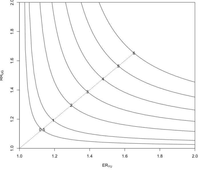
(0.34, 0.34).. . . 22 2.2 The equal-bias plot of ERY U and RRU G for the sexual behavior survey
data. The numbers on the curves denote the bias in standard er-ror units, with corresponding MinNI values (left to right) (1.13, 1.13), (1.19, 1.19), (1.30, 1.30), (1.39, 1.39), (1.48, 1.48), (1.56, 1.56), and
(1.65, 1.65).. . . 23 2.3 Isobols of E[Y]−E[Y|G= 1]in terms ofγ1 andβ1, fixingπ0 = 0.5. . . 24
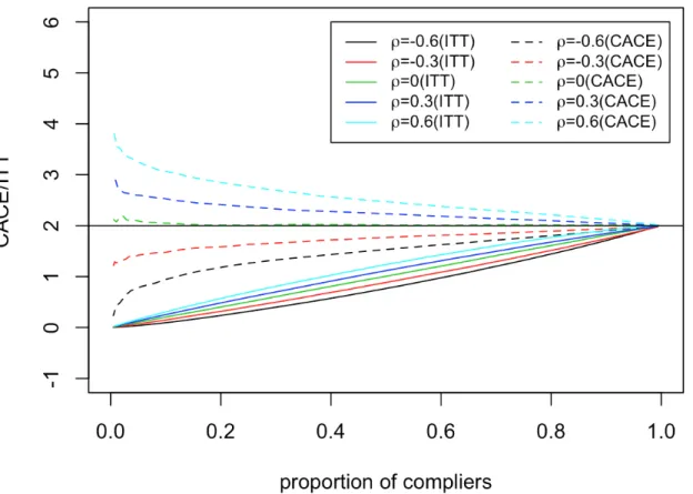
4.1 CACE and ITT(Y) as functions of ρ and the proportion of compliers for
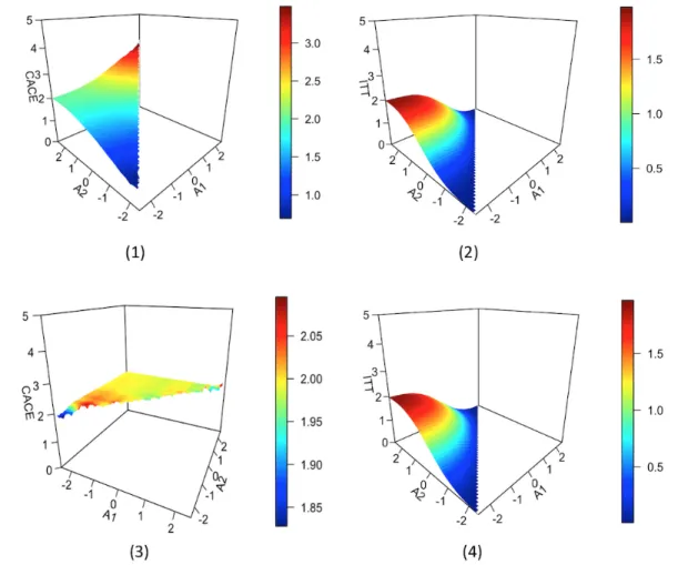
fixedτ = 2.. . . 50 4.2 CACE and ITT(Y) as functions of A1 and A2 for fixed τ = 2. (1) CACE
withρ = 0.6; (2) ITT(Y) withρ = 0.6; (3) CACE with ρ = 0; (4) ITT(Y)
LIST OF TABLES
Table Page
2.1 E[Y]−E[Y|G= 1]as a function of the sensitivity parameters.. . . 22
2.2 E[Y]−E[Y|G= 1]as a function of the sensitivity parameters withπ0 = 0.5. . . 23
2.3 The MinNI giving one standard error bias with different fractions of miss-ing data. . . 24
3.1 Sensitivity analysis for the slope in the smoking data, with artificially deleted data . . . 37
3.2 Missingness Patterns in the New York School Choice Experiment Data . . . 37
3.3 Sensitivity Analysis for the New York School Choice Experiment . . . 37
3.4 Sensitivity Analysis for the LA Endometrial Cancer Study . . . 38
4.1 The Sommer-Zeger vitamin A supplement data. . . 50
CHAPTER 1 INTRODUCTION
Incomplete data problems are encountered under various experiments, such as miss-ing responses in surveys, missmiss-ing outcomes or predictors in observational studies and noncompliance in randomized clinical trials. Each incomplete variable will induce one incompleteness mechanism; that is, the conditional distribution of the incompleteness in-dicators given the notional complete data. The ignorability conditions under which the stochastic nature of incompleteness mechanism could be ignored are of interest. How-ever, these conditions are hard or impossible to verify from the observed data and then, sensitivity analysis is one simple and appealing approach to assess the robustness of inferences when the ignorability conditions are violated.
1.1. Sensitivity analysis via unmeasured confounding
Rubin has elucidated the role of the missingness mechanism in extracting frequen-tist inferences from incomplete data [51]. The idea is to compare the distribution of the variables that are observed, conditional on the observed missingness indicators, to the marginal distribution of these same variables ignoring the missingness mechanism. The conditionmissing completely at random (MCAR)is sufficient to guarantee that these dis-tributions are identical, and therefore that the missingness mechanism is ignorable [36]. Briefly, MCAR requires that the conditional probability of the observed missingness indi-cators given the notional complete data is independent of the value of the complete data. Heitjan has extended this analysis to the coarse data model, where MCAR generalizes to
coarsened completely at random[22,23].
The Rubin approach begins with a selection model; that is, it parameterizes the joint distribution of the variable of interest Y and the missingness indicator G as the product of the marginal distribution ofY times the conditional distribution of Ggiven Y, denoting the latter the missingness mechanism. One can then identify ignorability conditions as restrictions on the parameters of the missingness mechanism. It is not possible to esti-mate the parameters of this joint model without strong assumptions [11]. An alternative, less ambitious, approach is to conduct sensitivity analyses to evaluate the robustness of estimates created under an ignorable model by re-estimating these parameters under a range of assumptions about the nonignorability parameters [9,38,58,60].
In the selection model, one describes the probability of missingness as a function of the potentially missing observation; if the missingness and the outcomes are correlated (conventionally, if a nonignorability parameter is nonzero), ignorability does not hold. As a practical matter, it may be preferable to consider the correlation to arise from confounding — as indeed may be the case — in that both the outcomes and the missingness indicators are associated with a third variable. If we can identify and measure this variable, a form of conditional independence holds that guarantees ignorability. If we cannot, we posit a form for it and consider the consequences of nonignorability on the distributions of measurable outcomes. Such models have long served as a basis for sensitivity analysis in observational studies, where the concern is that the treatment indicators and the potential outcomes are correlated in a way that biases standard causal analyses [10, 13, 33, 41,
1.2. Local sensitivity analysis for missing outcomes and predictors
A common model for data that are subject to missingness is the selection model. Ru-bin has elucidated conditions under which it is possible to ignore the stochastic nature of the missingness mechanism in Bayesian/likelihood inference [51]. Parameters distinct-ness (PD)asserts that the parameters governing the distribution of the notional complete data and the parameters governing the missingness mechanism lie in disjoint parame-ter spaces (for likelihood inference) or area priori independent (for Bayesian inference). Missing at random (MAR)requires that the missingness mechanism does not depend on the values of the missing items. MAR and PD are sufficient to guarantee the ignorabil-ity of missingness mechanism in likelihood-based and Bayesian analyses. Analyses that ignore the missing-data mechanism therefore implicitly assume MAR and PD [19, 28–
30,34,35,45,46,52]. PD is often plausible, but MAR is generally not, and moreover it is impossible to verify by analyzing the available data.
A subset of the parameters of the missingness mechanism serve as nonignorabil-ity parameters, in that they govern the association of the complete data values and the missingness. Typically, we parameterize such models so that the missingness mecha-nism is MAR when ignorability parameters are set to0. These parameters are impossible to estimate without strong assumptions, and even then, inferences may be numerically challenging and non-robust [11].
An alternative approach that is less ambitious but more practical is to evaluate the sensitivity of inferences to small departures from the MAR assumption; this is known as a local sensitivity analysis [9, 38, 58, 60, 64]. Such analyses to date have focused exclusively on situations where all missingness occurs in outcome variables, and none occurs in predictors. Moreover, in most such analyses there is a single nonignorability parameter, which considerably simplifies the interpretation of results. In Chapter 3, we extend an approach based on the index of local sensitivity to nonignorability (ISNI) [58]
to the setting with both missing outcomes and predictors. In the process, we develop a flexible index, the minimum nonignorability (MinNI), for interpreting local sensitivity when there are multiple sources of nonignorability.
1.3. Sensitivity of estimands in clinical trials with noncompliance
Many clinical trials exhibit substantial fractions of noncompliance to assigned treat-ments, leading to the problem of whether and how to incorporate compliance in trial analysis. After many years of discussion, clinical trialists settled on the as-randomized (AR) or intention-to-treat (ITT) analysis, which includes all subjects and groups them by the treatments to which they were randomized. The ITT estimate is unbiased for an es-timand that represents the effect of random assignment, rather than treatment received, on the outcome. Advocates of this approach argue that it is more pragmatic than alterna-tive analyses, as any attempts to assign treatments to a population will encounter some degree of noncompliance. A potential problem with ITT, however, is that it reflects the degree of noncompliance in the population under test; should compliance levels change — say, increasing over time to reflect growing recognition of a drug’s beneficial effects — the value of the estimand will also change.
Advocates of an approach to inference based on causal modeling have challenged this paradigm. A causal analysis takes a more structured approach to inference by first specifying the estimand of interest and then proceeding to identify conditions that render it estimable. For example, arguably the most important scientific estimand is the average effect of the treatment could all patients be compelled to comply with the randomization. Unfortunately, we cannot typically identify this estimand, known as thepopulation average causal effect (PACE), from randomized experiments with noncompliance [3, 14, 25, 57]. An alternative estimand is the complier average causal effect (CACE), defined as the average effect of the treatment in the latent subset of subjects who would comply with
their randomization assignment, whatever it is. Under five plausible assumptions it is possible to identify and estimate CACE from outcome and compliance data [2].
A problem with both ITT and CACE is that they explicitly reflect patient compliance behavior, which can vary with many factors related to the nature of the treatment and the characteristics of the persons administering and receiving it [8, 14, 43, 44]. For ex-ample, a systematic review of patient compliance in clinical trials has demonstrated that compliance levels for a particular drug can range from 40% to 74% depending on dose frequency [43]. Investigators have shown that educational interventions can raise com-pliance for a hypertension treatment from 36% to 42% [44]. Thus, it is plausible that estimands that incorporate compliance can be unstable, in the sense of reflecting varia-tion in compliance across formulavaria-tions, populavaria-tions, and time. In Chapter 4, we propose a novel assumption, “sixth assumption” to guarantee the robustness of CACE to random-ness of noncompliance class and conduct sensitivity analyses in a sumlation study and an illustrative real data example.
CHAPTER 2
SENSITIVITY ANALYSIS VIA UNMEASURED CONFOUNDING
In Section2.1, we describe the model and establish the general ignorability conditions. Section2.2presents a response-surface method for assessing variation of parameters of interest as a function of nonignorability parameters in a parametric model. In Section2.3, we adapt Cornfield’s paradigm, defining as an index of sensitivity the minimum magnitude of nonignorability that produces a designated level of bias. In Section 2.4 we apply the methods to incomplete data from a sexual behavior study. Section 2.5covers extensions of the approach.
2.1. Model and methods
2.1.1. Model and definitions
The data consist of an outcome variableY = (Y1, . . . , Yn)with corresponding vector of missingness indicatorsG= (G1, . . . , Gn), whereGi = 1forYi observed, andGi = 0for Yi
missing. Assume that an unmeasured variable U = (U1, . . . , Un)functions asconfounder in thatY andGareconditionally independent given U; that is, the conditional distribution ofY andGgivenU has the property that, for anyu,fY,G|U(y, g|u) =fY|U(y|u)fG|U(g|u)for allyandg. Thus, the joint density simplifies to
The confounding, if unmeasured or not accounted for, can induce correlation between
Y andG. Thus although we seek to create inferences for the marginal distribution ofY,
fY(y) = Z
fY|U(y|u)fU(u)du, (2.2)
in fact we may be only able to observe the conditional distribution ofY givenG=g:
fY|G(y|g) = R
fG|U(g|u)fY|U(y|u)fU(u)du
R
fG|U(g|u)fY|U(y|u)fU(u)dudy. (2.3) To this end, we establish restrictions on the conditional distribution terms in Equation (2.3) that are sufficient to guarantee ignorability, which in this context means that Equations (2.2) and (2.3) are the same. Throughout, we ignore any theoretical considerations about sets of measure0.
Theorem 2.1 Assume that either G ⊥⊥ U, or Y ⊥⊥ U. Then for any g such that fG(g) >
0, the distribution ignoring the missing mechanism in Equation (2.2) equals the correct distribution in Equation (2.3).
Proof. Suppose G⊥⊥U. Then∀g with0< fG(g)<1,
fY|G(y|g) = R fY|U(y|u)fG(g)fU(u)du R fY|U(y|u)fG(g)fU(u)dudy = R fY|U(y|u)fU(u)du R fY|U(y|u)fU(u)dudy =f Y(y).
Similarly, ifY ⊥⊥U, then∀g with0< fG(g)<1,
fY|G(y|g) = f Y(y)R fG|U(g|u)fU(u)du R fG|U(g|u)fU(u)du =f Y (y).
If Y or U is discrete, one can restate the theorem with summation substituted for integration. The ignorability condition in the theorem is stronger than MCAR because it applies to all possible missing patterns that have positive density, not just the observed
missing pattern [23,36]. In practice, the relevant conditional distribution will be the one for the outcome y conditional on the observed vector of missingness indicatorsg˜where the sample space ofywill be restricted to those which could agree with˜g, calledyconsistent with˜g. Thus, we develop an alternative, weaker version of Theorem2.1.
Consider the following conditions, assuming an observed valueg˜ofg:
1. The missingness isobserved ignorablein that for any possibleu,fG|Y,U(˜g|y, u)takes the same value for ally consistent withg˜.
2. fG|U(˜g|u)takes the same value for allu.
3. For anyyconsistent with˜g,fY|U(y|u)takes the same value for allu.
This leads to the following theorem:
Theorem 2.2 Under Assumption 1 and either of Assumptions 2 or 3, fY(y) = fY|G(y|g˜) for allyconsistent withg˜.
In practice, there may also be completely measured predictors. In such a case the theorems go through with appropriate conditioning, as shown in Section 2.5.3. These theorems offer the simplest general ignorability conditions for the confounding model. Ig-norability is generally not testable becauseU is typically hypothetical and Yi is available only when Gi = 1. Our idea therefore is to define nonignorability parameters in the con-text of Equation (2.1), then manipulate those parameters to determine how far they must depart from the ignorable model to create a substantial difference between fY(y) and
fY|G(y|g˜).
2.1.2. Sensitivity analysis in the confounding model
To simplify our exposition, we consider the situation where the data represent n in-dependently and identically distributed cases, with U a scalar unmeasured confounder.
Assuming that Y has finite mean and variance, we base our sensitivity analysis initially on a comparison of the marginal mean ofY to its mean conditional on its being observed. Theorems2.1 and2.2suggest that the sensitivity parameters can represent associa-tions between U andY and between U and G. We will describe two approaches: In the first, we depict bias conventionally by varying the nonignorability parameters over a plau-sible range based on a mildly parameterized model. This extends the sensitivity analysis of Rosenbaum and Rubin [50] from confounding in observational studies to nonignorably missing data. In the second, we consider a minimally parameterized nonparametric model and define the minimum nonignorability index (MinNI)to be the degree of nonignorability necessary to cause a non-negligible bias. This is similar to the Cornfield approach [10] to sensitivity analysis in observational research. As with all sensitivity analyses, ours de-pends in principle on the judgments of a hypothetical expert, whose role it is to identify the minimum non-negligible values of both the bias inY and the nonignorability parameters.
2.2. Response-surface sensitivity analysis
2.2.1. Sensitivity parameters
Assume first that the confounderU is binary. Then we partially specify the joint distri-bution of(Y, G, U)as
Pr[U = 0] =π0,
Pr[G= 1|U =u] =h(γ0+γ1u),
E[Y|U =u] =q(β0+β1u),
whereu ∈ {0,1} and h(γ0 +γ1u)and q(β0+β1u) are link functions. The parametersπ0,
observeU.
A standard approach to sensitivity analysis is to observe the change in a parameter of interest, in this case the marginal mean E[Y], as we vary the sensitivity parameters over plausible values. Under this model, the marginal and conditional means ofY in terms of these sensitivity parameters are, respectively,
E[Y] =q(β0 +β1)(1−π0) +q(β0)π0 (2.4)
E[Y|G= 1] = q(β0+β1)h(γ0+γ1)(1−π0) +q(β0)h(γ0)π0
h(γ0 +γ1)(1−π0) +h(γ0)π0
(2.5)
2.2.2. Estimation of means with specified nonignorability parameters
Under this model, Pr[G = 1] and E[Y|G = 1] are directly estimable from the data as
ˆ
p and µˆc, respectively. With π0, γ1, and β1 fixed, and observing a random sample of Y
values, some of which may be missing, one can readily estimate γ0 andβ0 [50]. The first
estimable term is
Pr[G= 1] =h(γ0 +γ1)(1−π0) +h(γ0)π0. (2.6)
Thus we have two Equations ((2.5) and (2.6)) and two unknowns (γ0andβ0). We calculate
the marginal mean in (2.4) as follows:
1. Solve Equation (2.6) forγˆ0, withpˆandπ0, γ1 fixed;
2. Solve Equation (2.5) for β0, with π0, γ1, β1 fixed, ˆγ0 from step 1, and µˆc estimated directly from the data;
3. Substitute βˆ0 andπ0, β1 into (2.4) to estimate the marginal mean.
AppendixA.1 presents details for the special case where both link functions are logistic, as would be applicable with a binary outcome.
Theorems 2.1 and2.2 assert that if γ1 = 0 or β1 = 0, there is no difference between
E[Y]and E[Y|G = 1]. Thus if small values of these parameters lead to substantial varia-tion in E[Y], we deem the results sensitive. If the response surface for E[Y]as a function of the sensitivity parameters is flat, then only large values of the sensitivity parameters imply non-negligible changes in E[Y|G= 1], and inferences are insensitive.
If the notional unmeasured covariate U is other than binary, the specification of the distribution forU is more complex and may involve more parameters. The distributions of
G given U and Y given U are indexed by link functions, whose specification induces an additional source of sensitivity. Thus, semiparametric or nonparametric models might be more satisfactory for this application.
2.3. Identifying the minimum non-negligible nonignorability
The response-surface analysis directly investigates the bias by mapping the effects of nonignorability on the distribution ofY. A complementary approach is to identify minimum values for the sensitivity parameters that yield a designated level of change — in this case, a pre-specified maximum negligible difference between E[Y|G = 1]and E[Y]. We denote these parameter values MinNI, for MinimumNonIgnorability. We seek moreover to conduct the analysis with a minimally parameterized model.
2.3.1. MinNI in the difference scale
Assume again a binary confounderU. We first note that
E[Y]−E[Y|G= 1] = (E[Y|G= 0]−E[Y|G= 1])Pr[G= 0]. (2.7)
Clearly, unless 0 < Pr[G = 0] < 1there is no need for a sensitivity analysis. Expanding the bias in Equation (2.7) in terms of the unmeasured confounderU, we observe that the
difference between E[Y|G = 0] and E[Y|G = 1] can be decomposed into the product of the difference between E[Y|U = 1] and E[Y|U = 0] and the difference between Pr[U = 1|G= 1]and Pr[U = 1|G= 0]. Details appear in AppendixA.2.
Define the sensitivity parameters as the two differences
EDY U =E[Y|U = 1]−E[Y|U = 0], RDU G=Pr[U = 1|G= 1]−Pr[U = 1|G= 0],
and observe that
|E[Y]−E[Y|G= 1]|=|EDY URDU GPr[G= 0]|. (2.8)
We can construct an insensitive region by specifying a maximum negligible difference for the bias as
|E[Y]−E[Y|G= 1]| ≤kσY|G=1, (2.9)
whereσY|G=1 is the standard deviation of Y given it is observed, and k is a positive
con-stant defined for the context, possibly related to sample size. From (2.8) and (2.9), we obtain the indifference region for the nonignorable parameters to be
|EDY URDU G| ≤
kσY|G=1
Pr[G= 0]. (2.10)
The Inequality (2.10) describes the relations among the maximum tolerable change and the sensitivity parameters. To define a single index of sensitivity, we identify the combina-tion of sensitivity parameters that satisfies this constraint and is closest to the origin. We
call this theMinNI for the mean. For a continuous outcome, the optimization process is Minimize: (ED2Y U +RD 2 U G) Subject to: |EDY URDU G| ≤ kσY|G=1 Pr[G= 0]; |EDY U| ∈(0,∞); |RDU G| ∈(0,1).
The closed-form feasible solution (i.e. MinNI) for (|EDY U|,|RDU G|) is
max ( kσY|G=1 Pr[G= 0], s kσY|G=1 Pr[G= 0] ) ,min ( 1, s kσY|G=1 Pr[G= 0] )! .
For a binary outcome, the range of|EDY U|in the optimization procedure is(0,1), and
MinNI= s kσY|G=1 Pr[G= 0], s kσY|G=1 Pr[G= 0] ! ,
wherekσY|G=1 ≤Pr[G= 0]. If MinNI is large, the sampling inference ignoring the missing
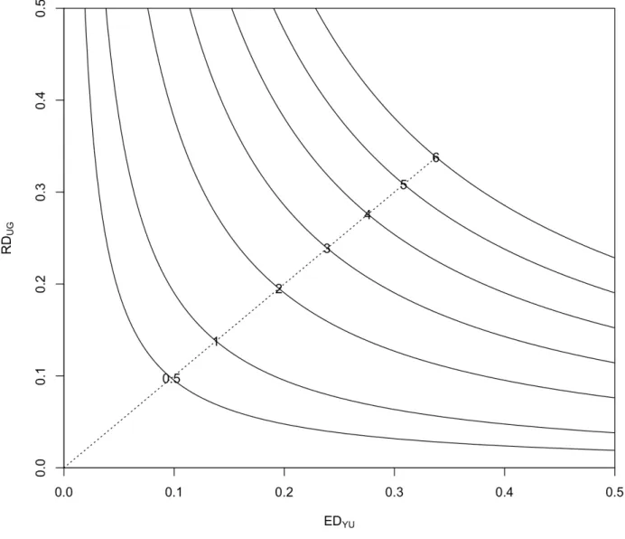
data is plausibly robust. If it is small, ignoring the missing mechanism could cause a considerable bias. Figure2.1illustrates the sensitivity analysis of the example discussed in Section2.4below.
2.3.2. MinNI in the ratio scale
For categorical variables, it might be preferable to describe bias on the ratio scale. Analogously with Equation (2.7), we observe that
E[Y]
E[Y|G= 1] =Pr[G= 1] +Pr[G= 0]
E[Y|G= 0]
where E[Y|G= 1]6= 0. Defining the nonignorability parameters as the ratios ERY U = E[Y|U = 1] E[Y|U = 0], RRU G= Pr[U = 1|G= 1] Pr[U = 1|G= 0], we obtain E[Y|G= 0] E[Y|G= 1] = ERY U −1 + Pr 1 [U=1|G=0] (ERY U −1)RRU G+Pr[U=11|G=0] . (2.12)
Because we cannot identify Pr[U = 1|G = 0], the best we can do is to obtain inequal-ities on the ratio in Equation (2.12), whose right-hand side is a monotone function of
1
Pr[U=1|G=0] ∈(RRU G,∞). We express the bounding inequality for the original ratio as
E[Y] E[Y|G= 1] −1 ≤ (ERY U−1)(RRU G−1) ERY URRU G Pr[G= 0], (2.13)
where ERY U ∈ (−∞,∞) and RRU G ∈ (0,∞). When Y is binary, we can specify an indifference region on the ratio scale by dividing both sides in (2.9) by E[Y|G = 1] to obtain E[Y] E[Y|G= 1] −1 ≤ |kCVY|G=1|. (2.14)
Here CVY|G=1 is the coefficient of variation ofY given that it is observed. The parameters
Pr[G = 0], σY|G=1 and CVY|G=1 are all estimable from the data. To be conservative, we
make the upper bound of the ratio in Inequality (2.13) less than the specified detectable difference from (2.14). The indifference region for the nonignorable ratio parameters is then (ERY U −1)(RRU G−1) ERY URRU G ≤ |kCVY|G=1| Pr[G= 0] (2.15)
of generality, that both ERY U and RRU Gexceed 1, the optimization process is Minimize: (ERY U −1)2+ (RRU G−1)2 Subject to: (ERY U −1)(RRU G−1) ERY URRU G ≤ |kCVY|G=1| Pr[G= 0] ; ERY U ∈(1,∞); RRU G ∈(1,∞).
The closed-form solution for (ERY U,RRU G) is then
MinNI= 1 1− r |kCVY|G=1| Pr[G=0] , 1 1− r |kCVY|G=1| Pr[G=0] ,
where |kCVY|G=1|< Pr[G = 0] ≤ 1. The interpretation is the same as for the difference
scale; see Figure2.2.
2.4. Sensitivity analysis for the Edinburgh sexual behavior survey
2.4.1. The data
Investigators surveyed 6,136 randomly selected students at the University of Edin-burgh in 1993. The parameter of main interest was the fraction responding “yes” to the question “Have you ever had sexual intercourse?”, which 2,308 students (37.6%) de-clined to answer [47, 58,62]. The observed proportion of positive responses, estimating E[Y|G = 1], is 0.7320 with standard error 0.0072. There is concern that nonresponders could have different patterns of sexual behavior compared to responders, potentially in-ducing a bias when estimating the parameter of interest. We describe below a sensitivity analysis for this proportion.
2.4.2. A response-surface sensitivity analysis
Table 2.1 displays the bias as a function of the sensitivity parameters, π0, β1, and γ1.
A plot of equal-bias contours inγ1 andβ1, with π0 fixed at0.5, appears in Figure2.3. We
fixedπ0 = 0.5because this value appears to give the largest bias.
In Table2.1, the absolute magnitude of the bias is modest as a fraction of the estimated parameter, reaching values no larger than about 3% on a relative scale. For purposes of statistical inference, however, the sensitivity is substantial, as the largest bias is roughly3
times the nominal standard error. The equal-bias plot in Figure2.3indicates that moder-ate values ofγ1andβ1can lead to2-SE changes to the mean. The analysis thus suggests
that estimation of the proportion of students who had had sexual intercourse is sensitive to nonignorability.
2.4.3. A MinNI sensitivity analysis compared with ISNI analysis
Here we set the maximum negligible bias to be 1 standard error of the observed proportion (here kσY|G=1 = 0.0072) and compute minimum values of the sensitivity
pa-rameters that produce this level of displacement. The MinNI for the difference scale, (EDY U,RDU G)=(0.14,0.14) from Figure2.1and for the ratio scale (ERY U,RRU G)=(1.19,1.19) from Figure2.2. The index is in both cases small, suggesting that the sampling inference for the true proportion of having sexual intercourse is sensitive. That is, even a mod-est disturbance from the ignorable model can induce a substantial bias into our mod-estimate of the population proportion, rendering tests and confidence intervals for this parameter unreliable.
We compare this analysis with an application of the likelihood-based ISNI (index of local sensitivity to nonignorability) sensitivity analysis [58, 62]. With ISNI, the key sen-sitivity statistic, denotedc, measures the approximate minimum standardized magnitude
of nonignorability needed to induce a 1-SE change in the maximum likelihood estimate of the parameter of interest. A value c < 1 is generally taken as evidence of sensitivity. For the proportion replying yes in the Edinburgh data, we computec= 0.097, suggesting strong sensitivity and agreeing with our frequentist analysis.
2.4.4. Dependence of MinNI on the fraction of missing data
Measures of sensitivity to nonignorability depend critically on the fraction of missing data; indeed the ISNI measure for a univariate normal mean with missing observations is proportional to the fraction missing [58]. To illustrate this relationship, we artificially varied the fraction of missing observations while holding the observed fraction of positive responses constant. We repeated the analysis with artificial missingness fractions set to 0.1 and 0.2, both smaller than the observed value of 0.376. Table2.2 shows the depen-dence of the bias for E[Y] as a function of the response-surface sensitivity parameters. Recalling that the standard error of the observed fraction of responses is0.0072, it is clear that for smaller fractions of missing data, sensitivity is modest except for the most extreme levels of confounding.
Table 2.3 shows MinNI values for the difference and ratio scale sensitivity analyses under the alternative fractions of missing observations. The interpretation of these values is that one would require weaker levels of confounding to induce a non-negligible bias in the observed fraction of positive responses.
2.5. Some extensions of the basic sensitivity analysis
2.5.1. A categorical confounder
withm >2levels. For the difference scale, denote the confounding relations as follows:
MDY U = max
i E[Y|U =ui]−mini E[Y|U =ui],
MDU G= max
i [Pr[U =ui|G= 1]−Pr[U =ui|G= 0]]. In AppendixA.3.1we derive the bounding inequality to be
|E[Y]−E[Y|G= 1]| ≤ |(m−1)MDY UMDU GPr[G= 0]|. (2.16)
To be conservative, we make the upper bound of the difference less than k standard deviations of the observed standard deviationσY|G=1,
|MDY UMDU G| ≤
kσY|G=1
(m−1)Pr[G= 0]. (2.17)
The dependence of the sensitivity on the number of categories is the same as found in Ding and VanderWeele (2014).
For the relative ratio scale, we denote the confounding parameters to be
ERY U(i)= E[Y|U =ui] min i E[Y|U =ui] , RRU G(i) = Pr[U =ui|G= 1] Pr[U =ui|G= 0] , MRY U = max i ERY U(i), MRU G = maxi RRU G(i).
Without loss of generality, we can take all of these parameters to be greater than 1. In AppendixA.3.1we show the bounding inequality to be
E[Y] E[Y|G= 1] −1 ≤ (MRY U −1)(MRU G−1) MRY UMRU G . (2.18)
This leads to the conservative indifference region
(MRY U −1)(MRU G−1)
MRY UMRU G
≤ kCVY|G=1
Pr[G= 0]. (2.19)
The corresponding MinNI derivations appear in AppendixA.3.2. 2.5.2. Sensitivity analysis for the variance
So far we have only considered bias in the mean of Y, but bias can also affect the variance. In an obvious notation, we defineσ2Bto be the variance of a random variableB,
potentially with conditioning. Setting
VDY U =σY2|U=0−σ2Y|U=1,VDU G=σU2|G=0−σU2|G=1, we obtain σY2 −σY2|G=1 = VDY URDU G+ED2Y UVDU G+ED2Y URD 2 U GPr[G= 1] Pr[G= 0]. (2.20)
Theorem2.1asserts that if G⊥⊥ U orY ⊥⊥U, then the difference in Equation (2.20) is 0. For the comparison of means, if either EDY U or RDU G is 0, there is no bias, but for the comparison of variance, this condition is not sufficient because VDY U or VDU G might not be 0. Commonly, the main moment of interest is the mean and it is shown that the first-order Taylor expansion ofσ2Y|G=1 is equal toσY2 [37,58]. We can readily derive analogous
results for estimating the conditional distribution ofY givenX. 2.5.3. Analysis with completely measured covariates
Many studies will include many baseline variables that, if unobserved, would confound the association of outcome and missingness; we denote such variablesX. We can readily generalize Theorems2.1and2.2to cover estimation of the distribution ofY givenX.
Theorem 2.3 Assume that Y ⊥⊥ G|(X, U) and that either G ⊥⊥ U|X or Y ⊥⊥ U|X. Then for any g andxsuch that fG,X(g, x) >0, the distribution ignoring the missing mechanism
fY|X(y|x), equals the correct distributionfY|G,X(y|g, x).
To generalize Theorem 2.2, we define the following assumptions, assuming that ˜g is the observed value ofG:
1. The missingness isobserved ignorable in that for any possibleuandx,
fG|Y,X,U(˜g|y, x, u)
takes the same value for allyconsistent with˜g.
2. For any possiblex,fG|X,U(˜g|x, u)takes the same value for allu.
3. For any possiblex and anyyconsistent with ˜g,fY|X,U(y|x, u)takes the same value for allu.
Theorem 2.4 Under Assumption 1 and either of Assumptions 2 or 3,
fY|X(y|x) =fY|X,G(y|x,g˜)
for allyconsistent withg˜.
Our analysis also readily generalizes to this situation; that is, by further conditioning on
X one can elucidate sensitivity as we have done above. Assume that the measured covariatesX are discrete. For the difference scale, denote the two confounding relations as
EDY U(X)=E[Y|X, U = 1]−E[Y|X, U = 0],
Therefore,
|E[Y|X]−E[Y|X, G= 1]|=|EDY U(X)RDU G(X)Pr[G= 0|X]|.
The above formula is similar to Equation (2.8). However, for the ratio scale, one naive analysis will be shown below.
E[Y|X]
E[Y|X, G= 1] =Pr[G= 1|X] +
E[Y|X, G= 0]
E[Y|X, G= 1]Pr[G= 0|X],
and we denote the relative ratios as
ERY U(X)= E[Y|X, U = 1] E[Y|X, U = 0], RRU G(X) = Pr[U = 1|X, G= 1] Pr[U = 1|X, G= 0]. Hence, E[Y|X, G= 0] E[Y|X, G= 1] = ERY U(X)−1 + Pr 1 [U=1|X,G=0] (ERY U(X)−1)RRU G(X)+Pr 1 [U=1|X,G=0] ,
which recalls Equation (2.12). All the other derivations follow directly. The total discrep-ancy between the marginal mean and the conditional mean after adjusting for theXcould be the summation of the discrepancy weighted byX.
Figure 2.1: The equal-bias plot of EDY U and RDU G for the sexual behavior survey data. The numbers on the curves denote the bias in standard error units, with corresponding MinNI values (left to right) (0.10, 0.10), (0.14, 0.14), (0.20, 0.20), (0.24, 0.24), (0.28, 0.28), (0.31, 0.31), and (0.34, 0.34).
Table 2.1: E[Y]−E[Y|G= 1]as a function of the sensitivity parameters.
π0 exp(β1) exp(γ1) 0.1 0.5 0.9 2 2 −0.0037 −0.0088 −0.0025 3 −0.0059 −0.0139 −0.0037 3 2 −0.0061 −0.0138 −0.0036 3 −0.0097 −0.0218 −0.0053
Figure 2.2: The equal-bias plot of ERY U and RRU G for the sexual behavior survey data. The numbers on the curves denote the bias in standard error units, with corresponding MinNI values (left to right) (1.13, 1.13), (1.19, 1.19), (1.30, 1.30), (1.39, 1.39), (1.48, 1.48), (1.56, 1.56), and (1.65, 1.65).
Table 2.2: E[Y]−E[Y|G= 1]as a function of the sensitivity parameters withπ0 = 0.5.
Fraction missing exp(β1) exp(γ1) 0.1 0.2 0.376 2 2 −0.0023 −0.0046 −0.0088 3 −0.0035 −0.0071 −0.0139 3 2 −0.0035 −0.0072 −0.0138 3 −0.0054 −0.0111 −0.0218
Figure 2.3: Isobols of E[Y]−E[Y|G= 1]in terms of γ1 andβ1, fixingπ0 = 0.5.
Table 2.3: The MinNI giving one standard error bias with different fractions of missing data.
Fraction missing
Scale 0.1 0.2 0.376
(|EDY U|,|RDU G|) (0.27,0.27) (0.19,0.19) (0.14,0.14) (ERY U,RRU G) (1.46,1.46) (1.28,1.28) (1.19,1.19)
CHAPTER 3
LOCAL SENSITIVITY ANALYSIS FOR MISSING OUTCOMES AND PREDICTORS
In Section 3.1, we derive expressions for ISNI and related statistics in the setting of missing data in outcomes and predictors, and describe an approach to interpretation. In Section 3.2, we derive the equations in the context of conditional logistic regression. In Section 3.3, we elucidate the index in a simple simulation study via artificial deleting. In Section3.4, we illustrate the index in two real-data applications involving the normal linear model and conditional logistic regression.
3.1. Methodology
3.1.1. ISNI
The data consist of independently and identically distributed copies of (Yi, Xi, Zi), i=
1, . . . , N, where Yi is the outcome, Xi is a predictor that is subject to missingness, and
Zi is a vector of predictors that are not subject to missingness. Gi andHi are indicators of whether Yi and Xi, respectively, are observed: Gi = 1(0) if Yi is observed (missing);
Hi = 1(0) ifXi is observed (missing). We can readily generalizeGi and Hi to vectors for
Denote the joint distribution for (Gi, Hi, Xi, Yi|Zi), fGi,Hi,Xi,Yi|Zi ξ,γ,θ,β (gi, hi, xi, yi|zi) =f Gi|Hi,Xi,Yi,Zi ξ (gi|hi, xi, yi, zi)fγHi|Xi,Yi,Zi(hi|xi, yi, zi) fYi|Xi,Zi θ (yi|xi, zi)f Xi|Zi β (xi|zi).
To simplify notation, we henceforth replace the symbolsfGi|Hi,Xi,Yi,Zi
ξ ,f
Hi|Xi,Yi,Zi
γ ,fθYi|Xi,Zi,
fXi|Zi
β byaξ,bγ,cθ,dβ respectively. The log likelihood is then
l = N X i=1 n higi[lnaξ(gi|hi, xi, yi, zi) + lnbγ(hi|xi, yi, zi) + lncθ(yi|xi, zi) + lndβ(xi|zi)] +hi(1−gi) ln Z aξ(gi|hi, xi, u, zi)bγ(hi|xi, u, zi)cθ(u|xi, zi)dβ(xi|zi)du + (1−hi)giln Z aξ(gi|hi, v, yi, zi)bγ(hi|v, yi, zi)cθ(yi|v, zi)dβ(v|zi)dv + (1−hi)(1−gi) ln Z aξ(gi|hi, v, u, zi)bγ(hi|v, u, zi)cθ(u|v, zi)dβ(v|zi)dudv o .
We denote the probabilities thatYi andXi are observed as, respectively,
aξ(1|hi, xi, yi, zi) = q(ξ0+ξ1xi+ξ2yi+ξ3zi+ξ4hi),
bγ(1|xi, yi, zi) = r(γ0+γ1xi+γ2yi+γ3zi),
where q and r stand for link functions. The primary parameter of interest isθ, which in-dexes the conditional distribution of the outcome Y given the predictors X and Z. The remaining parameters are nuisance parameters: β governs the distribtuion of X given
Z; γ = (γ0, γ1, γ2, γ3)governs the missingness mechanism ofX given X, Y, and Z; and
ξ = (ξ0, ξ1, ξ2, ξ3, ξ4)governs the missingness mechanism ofY givenH,X,Y, andZ. The
nonignorability parameters areν = (ξ1, ξ2, γ1, γ2)T, in the sense that ifν = 0, then the
miss-ingness mechanisms are missing at random (MAR). We moreover denoteξ0 = (ξ0, ξ3, ξ4)
and γ0 = (γ0, γ3) as the subsets of parameters of the missingness mechanisms that do
es-timated by maximum likelihood (MLE) when positing the nonignorability parametersν, as
(ˆθ(ν),βˆ(ν),ξˆ0(ν),γˆ0(ν)).
Troxel et al [58] introduced the index of local sensitivity to nonignorability (ISNI)as the basis of an analysis of sensitivity to nonignorability. Their idea is to assess the variability of the MLE of θ as a function of the nonignorability parameter in the vicinity of the MAR model. We extend their model, which assumes missingness only in the outcomeY, to the situation where both outcomes and predictors can be missing.
We begin by taking a first-order Taylor expansion of(ˆθ(ν),βˆ(ν),ξˆ0(ν),γˆ0(ν))atν = 0:
ˆ θ(ν) ˆ β(ν) ˆ ξ0(ν) ˆ γ0(ν) ≈ ˆ θ(0) ˆ β(0) ˆ ξ0(0) ˆ γ0(0) + ∂(ˆθ(ν), ˆ β(ν),ξˆ0(ν),γˆ0(ν))T ∂νT ν=0 ·ν.
Following [58], we define the index of local sensitivity to nonignorability as
ISNI= ∂(ˆθ(ν), ˆ β(ν),ξˆ0(ν),γˆ0(ν))T ∂νT ν=0 .
By the implicit function theorem, a general formula for ISNI is
− ∇2l θθ ∇2lθβ ∇2lθξ0 ∇2lθγ0 ∇2l βθ ∇2lββ ∇2lβξ0 ∇2lβγ0 ∇2l ξ0θ ∇2lξ0β ∇2lξ0ξ0 ∇2lξ0γ0 ∇2l γ0θ ∇2lγ0β ∇2lγ0ξ0 ∇2lγ0γ0 −1 ∇2l θν ∇2l βν ∇2l ξ0ν ∇2l γ0ν ν=0 ,
where∇2l
θθ is the second derivative of the log likelihood function with respect toθ under ignorable model, and other second derivatives follow similarly. We recognize the first fac-tor in ISNI as the variance-covariance matrix of (ˆθ,β,ˆ ξˆ0,γˆ0) under MAR, and the second factor as a measure of the orthogonality of (θ, β, ξ0, γ0)andν. The assumption of param-eter distinctness, i.e., that there are noa priori ties between(θ, β)and(ξ, γ), implies that
(∇2l
θξ0,∇2lθγ0,∇2lβξ0,∇2lβγ0) = 0under MAR. We present detailed formulas for calculating
ISNI in AppendixB.1.
3.1.2. Interpretation of ISNI
ISNI measures the degree of local sensitivity to nonignorability in the vicinity of the ig-norable model. Although ISNI is typically straightforward to compute, it is not invariant to such factors as the scale of measurement of continuous predictors. Therefore we propose a more flexible and interpretable index that evaluates the minimum degree of nonignor-ability required to cause a maximum negligible distortion in estimates of parameters of interest [7, 10, 33,41,50, 59,66]. Previous works have denoted such a measure as the
cindex [58].
Assume the nonignorability parameters ν is p-dimensional and each nonignorability parameter links one variable with missing to one missingness indicator. For example, in Section 3.1.1, ν is a 4-dimensional vector, (ξ1, ξ2, γ1, γ2)T, linking (xi, yi, xi, yi)T to these
missingness indicators in the nonignorable model. We denote the vector(xi, yi, xi, yi)T as the set ofcorresponding variables forν = (ξ1, ξ2, γ1, γ2)Tin the missingness mechanisms.
The vector of corresponding variables has the same dimension as the nonignorability parameterν.
The primary parameter of interest isθ. We denote
ISNI(ˆθ) =ISNI1(ˆθ), . . . ,ISNIi(ˆθ), . . . ,ISNIp(ˆθ)
where ISNIi(ˆθ)is the first derivative of θˆ(ν)with respect to thei-th nonignorability param-eter evaluated at ν = 0. If the i-th element in the corresponding variables is continuous, ISNIi(ˆθ)will be scale-dependent [58]. Denoteσ = (σ1, . . . , σp)for thepcorresponding vari-ables, where σi is the standard deviation of the corresponding variable if it is continuous, or 1 if it is discrete. The standardized ISNI is defined as
SISNI(ˆθ) = (SISNI1(ˆθ), . . . ,SISNIi(ˆθ), . . . ,SISNIp(ˆθ))
= (ISNI1(ˆθ)/σ1, . . . ,ISNIi(ˆθ)/σi, . . . ,ISNIp(ˆθ)/σp).
We define theminimum nonignorability (MinNI)to be the minimum degree of nonignor-ability that causes a maximum negligible distortion ofθˆ. As a default, we set the maximum negligible distortion to be the standard error (SE) ofθˆunder the MAR model. Xie and Heit-jan [63] proposed an extended ISNI in L2 space by Hölder’s inequality to approximately
measure the maximal sensitivity, and we transform it to minimum nonignorability as fol-lows:
MinNI= SE(ˆθ)
kSISNIk2
,
where
kSISNIk2= (SISNI1(ˆθ)2+· · ·+SISNIi(ˆθ)2 +· · ·+SISNIp(ˆθ)2)
1 2.
Algebraically, MinNI is approximately the radius of the smallest ball, centered at the MAR model, needed to produce a 1-SE change of θˆ. If MinNI is small, then the minimum nonignorability needed to distortθˆis plausible. That is, even modest nonignorability leads to sensitive estimates of parameters. If MinNI is large, only extreme nonignorability results in sensitivity.
Troxel et al [58] suggested a cutoff value 1 for c index, indicating that the minimal nonignorability to cause 1-SE displacement in θˆis that one unit change in outcome is associated with an odds ratio of 2.7 in the observation of probability. Similarly, we use
a cutoff value of 1 for MinNI, indicating that the minimum radius of a p-ball where the nonignorability parameters lie, needed to induce 1-SE distortion of θˆ is 1. That is, if MinNI<1, the sensitivity to nonignorable missing should be a serious concern.
As indicated above, Troxel et al [58] proposed the scale-independent sensitivity trans-formation orc value, which is an one-dimensional version of MinNI. Xie and Heitjan [63] proposed an index, SET, that is a two-dimensional version of MinNI that measures sen-sitivity to nonignorable treatment crossover in a randomized trial, where the crossover mechanism can differ by treatment arm. Chen [7] has proposed MinNI measures for the situation where missingness results from unmeasured confounders between the missing-ness indicator and the outcome. Although the unmeasured confounding specification in [7] differs from the selection model, the interpretations of sensitivity values are in the spirit of the proposal of Cornfield [10]. Our proposed MinNI includes thec value and the SET as special cases.
3.2. Conditional Logistic Model
3.2.1. Conditional likelihood
We apply the ISNI analysis to conditional logistic regression in matched case-control studies to assess the degree of local sensitivity when the predictors can have missing observations. The notation is the same as in Section3.1.1except that the outcomes are completely observed and the matched strata are defined by another set of completely observed variablesW. Suppose we have J strata, with stratum j containing1 case and
Mj controls. Subjecti in stratum J has data (hij, xij, yij, zij, wij) for i = 0,1, . . . , Mj and
j = 1, . . . , J. We denote subjecti= 0in each stratum to be the case. The total number of observations is stillN.
The joint distribution for (Yi, Xi, Hi|Zi, Wi) is, fYi,Xi,Hi|Zi,Wi(y i, xi, hi|zi, wi) =fγHi|Xi,Yi,Zi,Wi(hi|xi, yi, zi, wi)f Yi|Xi,Zi,Wi θ (yi|xi, zi, wi) fXi|Zi,Wi β (xi|zi, wi). Denote fHi|Xi,Yi,Zi,Wi γ (1|xi, yi, zi, wi) =r(1|xi, yi, zi, wi).
Without loss of generality, assumeX is discrete with a finite number of levels. We modify the parameterization for fYi|Xi,Zi,Wi
θ (yi|xi, zi, wi)f
Xi|Zi,Wi
β (xi|zi, wi) as in [52]. Define the odds of Y conditional on X, Z, W and the distribution of X conditional on Z, W in the control arm to be, respectively,
η(x, z, w) = Pr[Y = 1|X =x, Z =z, W =w]
Pr[Y = 0|X =x, Z =z, W =w],
π(x|z, w) = Pr[X =x|Y = 0, Z =z, W =w].
After we specify models forηandπ, the other two functions are determined:
˜ η(z, w) = Pr[Y = 1|Z =z, W =w] Pr[Y = 0|Z =z, W =w] = X v η(v, z, w)π(v|z, w); ρ(x|z, w) = Pr[X =x|Y = 1, Z =z, W =w] = π(x|z, w)η(x, z, w) ˜ η(z, w) .
The conditional likelihood for the1:Mj matched case-control study is
L= ( J Y j=1 ˜ η(z0j, w0j) Mj P k=0 ˜ η(zkj, wkj) ) N Y i=1 ( π(xi|zi, wi)(1−yi)ρ(xi|zi, wi)yir(1|xi, yi, zi, wi) )hi ( X v π(v|zi, wi)(1−yi)ρ(v|zi, wi)yi[1−r(1|v, yi, zi, wi)] )1−hi .
3.2.2. Model specification
For brevity, assume that X is binary. Define
η(x, z, w) = exp{θ0(w) +V(x, z, w)Tθ}
and
π(x|z, w) = exp{xU(z, w)
Tβ}
1 + exp{U(z, w)Tβ}. Thus, the score functions forθ andβ under MAR are,
N X i=1 ( V(xi, zi, wi)yihi+ ˆV(zi, wi) [yi(1−hi)−Yc(zi, wi)] ) = 0, (3.1) N X i=1 ( [yi−Yc(zi, wi)] ˆU(zi, wi) +hiU˜(xi, zi, wi)−yihiUˆ(zi, wi) ) = 0, (3.2) where ˜ U(xi, zi, wi) = (−1)1−xi(1−π(xi|zi, wi))U(zi, wi), ˆ V(zi, wi) = X v V(v, zi, wi)ρ(v|zi, wi), Yc(zi, wi) = ˜ η(zi, wi) Mj(i) P k=0 ˜ η(zk,j(i), wk,j(i))
withj(i)meaning thej-th strata where thei-th observation belongs to, and
ˆ
U(zi, wi) =
X
v
(−1)1−vρ(v|zi, wi)(1−π(v|zi, wi))U(zi, wi).
We can solve the score equations (3.1) and (3.2) simultaneously through quasi-Newton algorithms with numerical Hessian [6,16,18,53]; this enables us to compute the first
fac-tor of ISNI. Assumingr is a logistic link, the terms in the second factor of ISNI are ∂2l ∂θ∂γ1 γ1=0 = N X i=1 −(1−hi)ri yi X v vρ(v|zi, wi)(V(v, zi, wi)−Vˆ(zi, wi)) , ∂2l ∂β∂γ1 γ1=0 = N X i=1 −(1−hi)ri ( yi X v vρ(v|zi, wi) ˜ U(v, zi, wi)−Uˆ(zi, wi) + (1−yi) X v vπ(v|zi, wi) ˜U(v, zi, wi) ) , where ˜ U(v, zi, wi) = (−1)1−v(1−π(v|zi, wi))U(zi, wi), ri = exp{γˆ0+ ˆγ2yi+ ˆγ3zi+ ˆγ4wi} 1 + exp{γˆ0 + ˆγ2yi+ ˆγ3zi+ ˆγ4wi}
under MAR. Then, plug all the estimations into ISNI formula and modify it to MinNI as defined in Section3.1.2.
3.3. Simulated Missing Observations in the Smoking and Mortality Data
We illustrate our proposed ISNI and MinNI by artificially deleting observations from a complete data set. The data are from a smoking and mortality study of English men grouped into 25 occupational categories [42]. There are two variables: The smoking index (the predictor) is the ratio of the average number of cigarettes smoked per day by men in the occupational group to the average number of cigarettes smoked per day by all men; the mortality index (the outcome) is the ratio of the rate of deaths from lung cancer among men in the occupational group to the rate of deaths from lung cancer among all men. The slope in a linear regression is 1.088 with SE 0.221.
To systematically delete observations, we first order the data according to the values of the smoking index and then, delete the smoking index points sequentially by ranks. Similarly, we order the data by the mortality index to perform deleting of the mortality
index. We construct four types of missing patterns: A single point missing on mortality index with a single point missing on smoking index; a single point missing on mortality index with five points missing on smoking index; five points missing on mortality index with a single point missing on smoking index; and five points missing on mortality index with five points missing on smoking index. Assume the smoking index and the mortality index follow a bivariate normal distribution. We present the most and least sensitive cases of each type in Table3.1.
In the first missingness type, the least sensitive case is the one that omits point 7 of the mortality index and point 21 of the smoking index. This gives a MinNI of 80.148, which says that the minimum radius of a4-ball of vectors of nonignorability parameters needed to cause 1 SE change in the slope estimation is 80.148. This suggests the needed minimum nonignorability is implausible and thus the MLE estimation of the slope is insensitive. The most sensitive case omits point 1 of the mortality index and point 2 of the smoking index, giving a MinNI of 1.639.
The least and the most sensitive cases with their MLEs, standard errors and MinNIs under the second, third and fourth types missingness types appear in rows three to eighth of Table3.1. When we move from the first type to the fourth type, the MinNIs for the least sensitive case are decreasing(i.e. the estimates getting more sensitive) as the proportion of missing values increasing. Generally, when data are missing toward the middle of the range of smoking status, sensitivity is modest, because the missing points have low leverage and cannot readily influence estimation of the slope. Conversely, when missing points are at the edge of the range of smoking status, sensitivity can be substantial, because these are points of high influence [58].
3.4. Real-Data Examples
3.4.1. The New York School Choice Experiment
The New York School Choice Experiment, conducted in 1997, sought to estimate the effect of vouchers to attend private school on the academic performance of children from low-income families in New York City [4, 27]. The data consist of 525 selected children and 525 matched controls with a list of predictor variables spanning educational, demo-graphic, and socioeconomic indicators and baseline academic performance. The out-come variables were reading and math scores in the school year after the randomization. See more details about the data in [27].
To illustrate our method, we will take the math score to be the outcome variable, with all the other variables as predictors. The model is a multivariate normal linear regres-sion. We conducted a complete-case analysis using elastic net regularization to identify a small subset of strong predictors. We used default settings of the cv.glmnet function inR package glmnet [17]. The analysis identified as important predictors the grade level and the pre-test math score. We also included the randomization indicator, as the main purpose of the study was to evaluate its effect. The missingness patterns for the full data set (including both complete and incomplete cases) appear in Table3.2.
Assume the distribution for the pre-test and the post-test math scores conditional on grade level and randomization follows bivariate normal. We estimated coefficients of the regression of post-test math score on pre-test math score, three indicators of grade level, and randomization indicator. First we conducted a complete-case analysis, as shown in Column 2 of Table 3.3. Next we computed the maximum likelihood estimate of the coefficients using the full data set, integrating the density over missing observations to obtain the likelihood function under MAR; see Column 3 of Table 3.3. Corresponding MinNI values for the regression coefficients apper in Column 4.
All MinNIs for these predictors are greater than 1, but the one for randomization is close to 1. The coefficient of randomization measures the encouragement effect of being offered a voucher on math scores. Thus the estimated effect from complete cases and un-der MAR, which are of borun-derline significance, are potentially sensitive to nonignorability. The SISNI vector for lottery status is (−0.051,−0.902,0.065,0.103)T. The largest magni-tude of the elements in this SISNI vector is 0.902, corresponding to the missing post-test math score in the missingness mechanism for the post-test math score. The main contri-bution to the overall local sensitivity on the parameter estimation of lottery status is from the missing post-test math score in the missingness mechanism for the post-test math score.
3.4.2. The Los Angeles Endometrial Cancer Case Control Study
This was a 1:4 matched case-control study that investigated the effect of various risk factors on endometrial cancer, conducted among residents of the Leisure World retire-ment community. Investigators matched 63 cases to 4 controls each by date of birth, mar-ital status, and residence [39,52]. The explanatory variables of interest are GALL (history of gall bladder disease), OB (obesity), and EST (history of use of estrogen therapy). Only OB has missing observations, with 50 (16%) of the values unobserved. Because no strat-ification variables are available in the data set, we assumed thatπ(x|z, w)did not depend onw.
Table3.4displays the complete-case and maximum likelihood estimates of the regres-sion coefficients, together with ISNI and MinNI values. All the MinNIs are greater than 1. But in this case several of the predictors are relatively sensitive to potential nonignorabil-ity compared with other predictors, including main effects and interactions involving OB but also other main effect EST. In particular, inferences regarding the effects of OB, EST, OB×GALL and OB×EST in this data should be regarded with caution.
Table 3.1: Sensitivity analysis for the slope in the smoking data, with artificially deleted data
Missing Mortality Ranks Missing Smoking Ranks MLE SE MinNI
7 21 1.026 0.211 80.148 1 2 0.815 0.261 1.639 16 14-18 1.120 0.214 349.218 5 1-5 0.433 0.349 0.472 5-9 12 1.112 0.204 371.535 1-5 5 0.505 0.343 0.415 9-13 6-10 1.277 0.251 64.804 5-9 1-5 0.261 0.268 0.303
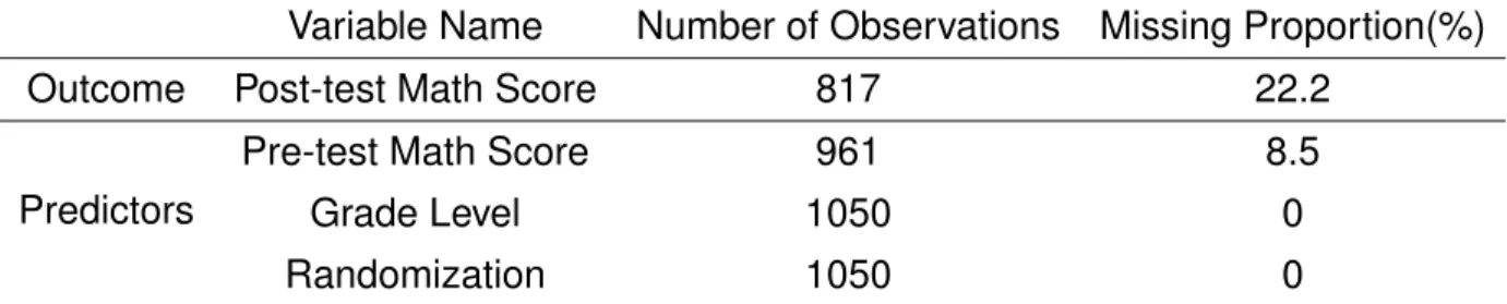
Table 3.2: Missingness Patterns in the New York School Choice Experiment Data Variable Name Number of Observations Missing Proportion(%)
Outcome Post-test Math Score 817 22.2
Predictors
Pre-test Math Score 961 8.5
Grade Level 1050 0
Randomization 1050 0
Table 3.3: Sensitivity Analysis for the New York School Choice Experiment
Variable Complete case (SE) MLE under MAR (SE) MinNI Pre-test Math Score 0.418 (0.033) 0.416 (0.033) 5.648 Grade Level(2) −3.248 (1.657) −3.195 (1.636) 5.491 Grade Level(3) 5.964 (1.638) 6.322 (1.624) 2.190 Grade Level(4) 1.355 (1.873) 1.791 (1.822) 4.436 Randomization 1.922 (1.216) 2.157 (1.197) 1.313
T ab le 3.4: Sensitivity Analysis for the LA Endometr ial Cancer Study V ar iab le Complete case MLE(SE) Conditional Logistic MLE under MAR(SE) ISNI MinNI OB 1.460(1.381) 1.291(1.584) 0.521 3.039 GALL 3.256(1.282) 2.897(1.103) 0.202 5.463 EST 3.531(1.395) 3.200(1.451) 0.454 3.195 OB × GALL − 0.146(0.914) − 0.087(0.665) − 0.180 3.686 OB × EST − 1.116(1.389) − 0.762(1.603) − 0.507 3.162 GALL × EST − 2.270(1.168) − 2.020(0.936) − 0.075 12.482
CHAPTER 4
SENSITIVITY OF ESTIMANDS IN CLINICAL TRIALS WITH NONCOMPLIANCE
In Section 4.1, we supplement the basicRubin causal model (RCM) for a clinical trial to reflect potential association between compliance and outcome. Within this framework, we illustrate the effect of compliance on the ITT and CACE estimands. We moreover demonstrate a condition, which we denote the “sixth assumption”, that is sufficient to render CACE robust to such variation. This assumption is plausible though unverifiable in any single study, but with our model one can readily conduct analyses to illustrate sensitivity to its violation. In Sections 4.2 and 4.3, we illuminate such analyses through simple simulation studies and a trial of vatamin A supplementation in children.
4.1. Clinical Trial Estimands
4.1.1. The RCM: Notation
Consider a population with N experimental units, i = 1, . . . , N, whom we will ran-domize between two study arms. Denote the N-vector of randomization assignments
Z = (Z1, . . . , ZN), where Zi = 1(0)indicates assignment of subject ito the experimental
(control) arm. In many clinical trials, subjects can exercise some control over the treat-ment they receive, in which case the treattreat-ment received may not match the treattreat-ment assigned. Thus, the assignment vectorZ gives rise to a further N-vector of actual treat-ments received D=D(Z)withi-th elementDi(Z). Here,Di(Z) = 1(0) indicates that, for treatment assignment vectorZ, unit i receives the experimental (control) treatment. The
outcome is denoted as Y = Y(Z, D) with Yi(Z, D(Z)) indicating the i-th outcome value given the assignmentZ and the treatment receivedD(Z).
Note that both the treatment received and the outcome are potential outcomes, in that there are as many potential N-vectors D(Z) and Y(Z, D(Z)) as there are values of the randomization vector Z. If, as is often the case, there is no interference between units, it is possible to make the stable unit treatment value assumption (SUTVA) (see Section4.1.2), which asserts thatDi(Z) = Di(Zi) andYi(Z, D(Z)) =Yi(Zi, Di(Zi)). This greatly simplifies the model, because we need to consider only two potential values of the treatment received — Di = (Di(0), Di(1)) — and four potential values of the outcome —
Yi = (Yi(0,0), Yi(0,1), Yi(1,0), Yi(1,1)). Moreover, among the four potential outcomes inYi we need consider only the two that can actually arise: Yi(0, Di(0))andYi(1, Di(1)).
Considering the various patterns of Di(0) and Di(1) leads to four principal strata of compliance behaviors; we denote this variableTi(Di):
Ti = n(“never-taker”), if(Di(0), Di(1)) = (0,0); c(“complier”), if(Di(0), Di(1)) = (0,1); a(“always-taker”), if(Di(0), Di(1)) = (1,1); d(“defier”), if(Di(0), Di(1)) = (1,0).
Subjectihas a vector of data(Zi, Di(0), Di(1), Yi(0, Di(0)), Yi(1, Di(1))), of which only the three elements (Zi, Di(Zi), Yi(Zi, Di(Zi))) are observable. We define Dobs to be the N -vector of treatment taken Dobs = D(Z), and the realized outcome of interest as Yobs =
Y(Z, Dobs). In the basic RCM, the sole random element isZ; the other variables are fixed but possibly unknown constants, analogous to the role of outcome variables in design-based sampling theory [2,31,32].
![Figure 2.3: Isobols of E[Y ] − E[Y |G = 1] in terms of γ 1 and β 1 , fixing π 0 = 0.5.](https://thumb-us.123doks.com/thumbv2/123dok_us/9022769.2800136/37.918.112.805.191.640/figure-isobols-e-y-e-y-terms-fixing.webp)