How wide is the gap?
An investigation of gender wage differences using quantile regression.
Jaume García∗∗∗∗ Pedro J. Hernández† Angel López-Nicolás∗∗∗∗
We thank Manuel Arellano, Richard Blundell, Adriana Kugler and seminar participants at Universitat Pompeu Fabra, Universitat de Girona, Universidad de Oviedo, the XII Jornadas de Economía Industrial and the XV Latin American Econometric Society Meeting for suggestions. We are also grateful to the editor of this journal and an anonymous referee for useful comments. Financial support from the Instituto de la Mujer, the FIES and DGES projects PB95-0980 and PB98-1058-C03-01 is gratefully acknowledged. The usual disclaimer applies.
∗∗∗∗Departament d’Economia i Empresa. Universitat Pompeu Fabra
†Departamento de Fundamentos del Análisis Económico. Universidad de Murcia.
Address for correspondence: Jaume García
Department of Economics and Business Universitat Pompeu Fabra
Ramón Trias Fargas, 25 08005 Barcelona Spain
Tel + 34 3 5421748 Fax + 34 3 5421746
Introduction
The wage gap between men and women in Spain, in line with what happens in
other countries, is quite substantive. Data from the 1995 Encuesta de Estructura
Salarial show that on average women earn around 70% as much as men. 1 This difference cannot be accounted for by observable variables such as experience, sector of employment or education. Indeed, when the wage gap is computed by levels of education, the same survey reveals that women who have completed a university degree earn on average a 60% of the salary received by men with the same educational level. The degree to which observed differences in salaries between men and women can be accounted for by observable characteristics has been a subject of interest in the labour economics literature, not least because unexplained differences have been interpreted as a degree of wage discrimination against women.
The usual methodological approach in the studies that attempt to measure it consists in decomposing the wage gap into a part attributable to differences in the vector of worker characteristics and a part attributable to differences in the return associated to each of these characteristics using the estimates for the expectation of the conditional
wage distribution of both groups.2 The most recent results obtained with this
methodology for the Spanish labour market are found in the works by Riboud and Hernández (1989), Ugidos (1993), Hernández (1995, 1996, 1997), de la Rica and Ugidos (1995), Prieto (1995) and Ullibarri (1996). Even if the data sources and
1
The unemployment rate for Spanish women, at 30%, doubles that of men.
methodologies applied are different, all these studies find that a substantial percentage of the wage gap is due to differences in the returns to observable characteristics in
favour of men. Results for other countries detect the same qualitative pattern.3
However, an important limitation of this methodology is that disregarding the information that other functions of the wage distribution provide may lead us to conclude that the size of the wage gap and the weights of the factors that make it up are constant along the whole of the wage scale. Stemming from the seminal work of Juhn et al. (1993), recent examples in the literature address this issue by analysing differences between quantiles of the wage densities of not only men versus women but also different countries or different points in time for a given population. For instance, Di
Nardo et al. (1996)model the wage distribution using non parametric kernel reggression
methods. Thus these authors and are able to gauge the extent to which changes in the distribution of worker characteristics can account for changes all over the wage density. In two related studies, Fortin and Lemieux (1998), using rank regression methods, and Machado and Mata (1999), by means of a quantile regression model and bootstrapping techniques, model the marginal wage distribution as a function of worker characteristics. Since these studies parameterise the relationship between wages and skills, the authors are able to measure not only the impact of differences in the distribution of skills but also the effect of differences in the return to these skills on the percentiles of the wage densities. The evidence that arises from these studies strongly suggests that average wage gaps and decompositions are not representative of the gaps
3
See Neumark (1988), Wright and Ermisch (1991), Callan and Wren (1994), Harkness (1996) and Blau and Kahn (1992, 1997) among others.
(and factors that explain these gaps) between different quantiles of the wage distributions for the populations of interest.
In this paper we argue that there is a clear link between the unequal size of the gender wage gap over the wage scale and the concern in the literature about the partial ability of traditional discrimination measures based on wage expectations to capture the full extent of the phenomenon of discrimination. Kuhn (1987) pointed for the first time at this limitation and supported it with evidence about the lack of a significant relationship between the traditional statistical measures of discrimination and reports of discrimination on behalf of women. Other researchers have reported results along the
same lines.4 According to Kuhn, the key determinant of this result is the mismatch
between what the researcher observes in the data set and the much richer information set at the disposal of the worker.
The main contribution in this paper consists in showing the ability of the quantile regression conceptual framework to compensate such mismatch. Thus we shall propose and justify the use of quantile regression models and the decomposition of predicted wage gaps at diverse quantiles in order to provide a more accurate set of measures for the size of the part of the wage gap that is attributed to different returns to skills between men and women, i.e. the discriminatory component of the wage gap. As we shall argue, our results are consistent with the evidence reported by Kuhn (1987) about the higher likelihood of reporting being discriminated against on behalf of women at high wage levels. Thus our evidence would suggest reconciliation between
“objective” and “subjective” measures of discrimination. Indeed, an interesting issue in the research agenda in the area of wage discrimination originates from the results in this paper. It consists in the examination of the statistical relationship between objective measures of discrimination, obtained from the decomposition of quantile functions, and subjective reports on behalf of the concerned worker using suitable data sets, i.e. data sets that contain not only the usual information on wages and characteristics but also subjective reports of discrimination.
The analytical framework we adopt for the estimation of conditional quantile functions is based on the quantilic regression methodology developed by Koenker and Basset (1978) and applied, in the context of wage equations, by Chamberlain (1994), Poterba and Rueben (1994), Buchinsky (1994, 1996, 1997), Machado and Mata (1999) and, for the Spanish case, Abadie (1997). In our analysis we shall pay special attention to the way in which one of the key variables determining wages, schooling, enters the econometric specification. Many of the studies that analyse the wage gap, including all those available for the Spanish labour market, take education as an exogenous variable.
However, as several recent studies have shown,5 the correlation of schooling with
unobserved factors that enter the determination of wages can produce inconsistent
estimates.6 The decomposition of the wage gap into the explained and unexplained parts
relies on the availability of unbiased estimates of the returns to a series of
4
See Hallock et al. (1998).
5 See Angrist and Krueger (1991), Neumark and Korenman (1994) , Harmon and Walker (1995, 1996) or
the review in Card (1994).
characteristics.7 Therefore, we use instrumental variables techniques in the estimation of both the conditional mean and conditional quantile functions. The corrections of the biases induced by the endogeneity of education in the context of quantile regression are based on the results by Amemiya (1982) and Powell (1983). Another relevant issue from the methodological point of view is the problem of endogenous selection of women into the labour force. The traditional Heckman method is applied when we estimate the conditional mean for wages. Correspondingly, in order to estimate the quantile regression model we use the results by Buchinsky (1996) to correct the associated bias. To the best of our knowledge this is the first application of quantile regression methodology where the issues of endogeneity of education and endogenous selection into the labour market for women are addressed simultaneously.
In addition, our methodology is related to that used in studies devoted to analysing the sources of overall wage inequality such as Machado and Mata (1999). Thus our empirical results cast some light on what factors are associated to a greater wage dispersion as well as how these factors vary in importance across genders for Spanish workers.
In section 2 we develop the argument in favour of the use of quantile regression based measures of discrimination and present the econometric specification used throughout the paper. Section 3 discusses the data set and the set of instruments used to correctly identify the parameters in the wage equation. Section 4 presents and discusses
7
The impact of potential biases on the decomposition of wage differentials are analysed in Kim and Polachek (1994) and Choudury (1994).
the econometric estimates, which are then used to evaluate and decompose the wage gap over the wage distribution in section 5. Section 6 concludes.
2. Econometric specification
2.1 Why should we be interested in anything but conditional wage expectations?
As we have mentioned in the introduction, Kuhn (1987) found evidence that the standard measures derived for the gender wage gap are not able to capture perfectly the
extent of discrimination as it is perceived by the concerned worker.8 More precisely, he
could not find a statistically significant association between the probability of reporting discrimination and the wage gap that separated women from men of equal characteristics using two different data sets. According to Kuhn, the tendency to report discrimination depends on “non statistical evidence” (in the sense that it is not observable by the analyst). The latter comprises any differential treatment at the workplace as well as any information on wage discrimination not captured by the standard measure based on estimates of the conditional mean of wages for men and women. It is this latter component of “non statistical evidence” that we concentrate upon.
The standard measure of discrimination is based on the following (mean) regression model for the logarithm of wages
ln( ) ln( ) ' ' W X u W X u m m m m f f f f = + = + β β (1)
where the m and f subscripts refer to males and females respectively. As it is well
known, from the first order conditions of OLS and using the male wage structure as non-discriminatory, it follows that
ln(Wm)−ln(Wf)=(Xm− X f)'β!m− X'f(β!m −β!f )
(2)
where the first term in the right hand side represents that part of the percentage difference between male and female average wages due to the different characteristics males and females have, whereas the second term is the part attributable to the existence
of differential returns to the same characteristics.9 From this decomposition Kuhn,
considers the following individual measures of discrimination for every woman in the sample ! ( ! ! ) ! ( ! ! ) ! D X D X u i if m f i if m f if 1 2 = ′ − = ′ − − β β β β (3)
The only difference between these two alternative measures is that the second
takes into consideration the return to the unobserved characteristics of the ith woman. In
8 See also Barbezat and Hughes (1990), Even (1990) and Kuhn (1990). 9
As it is shown in Hernández (1995), the results for the Spanish case are robust to different assumptions about the non-discriminatory wage structure.
this sense the latter measure is more related to the subjective perception of discrimination than the first one, for women make inferences conditional on a wider set of information than that observed by the econometrician. Indeed, among the factors picked up by the residual, there will typically be the unobserved productivity components and firm fixed effects which, in conjunction with the usual purely random
component, place the ith unit of observation above or below the conditional expectation
estimated by the researcher.
Our contribution to the argument starts here. It hinges on the point that women will infer the extent of their wage discrimination by comparing themselves with men who also have these (unobserved to the econometrician) characteristics. For instance, among the workers with an university degree, a characteristic which econometricians can usually observe, some will work at firms which reward computer literacy and/or knowledge of languages, but the econometrician usually cannot observe neither whether the firm rewards such skills nor which worker has them. In these circumstances, it is reasonable to expect women to form an idea of the discrimination that they may suffer comparing themselves not just with the group of workers with a degree, but with the group of workers with a degree at the same firm and with the same mastery of computers and languages. We define a measure of wage discrimination that takes this reasoning into account
! ( ! ! ) * !
Di3 = ′Xif βm−βf +uim −uif
(4)
where the term uim* is the effect of the unobserved factors on the wage of a man with the
consideration of this measure would in fact constitute a way to make regression based measures of discrimination more complete since they would capture a substantial part of the wage discrimination comprised in the “non statistical evidence” which Kuhn reported to drive subjective reports.
Concerning the computation of this measure, it is unfortunate that we cannot
estimate uim*. However, by the reasoning above we can argue that its sign is the same as
that of u!if. That is, women with unobserved characteristics that situate their wage above
the expectation of wages conditional on their observed characteristics will compare themselves with men whose wage would be situated above the expectation of male wages conditional on the same observed characteristics. This immediately suggests the comparison of quantiles of the two wage distributions conditional on the same set of characteristics as an approximation to the essentially unobservable measure we have
defined above. Thus, for any set of observable characteristics Xi, the women who
receive the wage that leaves behind a fraction θ of women with the same observable
characteristics may be compared with the men who, with the same observable
characteristics, earn a wage that leaves behind a fraction θ of men in the same group by
means of the following
(5)
where Qθ(log W | Xi) represents the θ quantile of the wage density conditional on Xi.
This approximation therefore requires obtaining estimates of the conditional quantile functions of the wage densities for men and women.
(
)
(
)
ˆ3 | log ˆ | log ˆ Wm Xi Q Wf Xi Di Qθ − θ ≅2.2 The quantile regression model
The basic quantile regression model specifies the conditional quantile as a linear
function of covariates10. For the conditional wage distribution we are examining, the
formal econometric representation is given by (omitting gender subscripts)
log (log | ) log ' ' W X u Q W X W X i i i i i i i = + = = β β θ θ θ θ θ (6)
and therefore it is assumed that the θth quantile of the error term which, as discussed
earlier, contains both fixed unobservable effects and pure random elements, is zero. Under this representation, the measure of discrimination in equation (5) is given by the following expression
(7)
The estimates for the conditional quantile functions can also be used to decompose the differences in quantiles of the marginal densities. The properties of the OLS estimators ensure that the predicted wage evaluated at the sample average vector of
10 With this specification we are also taking into account the potential existence of heteroscedasticity of
the form considered in Rutemiller and Bowers (1968), i.e. that the variance of the error term is a quadratic form of the regressors.
(
)
(
)
(
ˆ ˆ)
ˆ3 | log ˆ | log ˆ Wm Xi Q Wf Xi Xi m f Di Qθ − θ = ′ βθ −βθ ≅characteristics is exactly equal to the sample average wage but, unfortunately, the estimators for the quantile regression model do not have any comparable property. Therefore, the difference between two quantiles of the marginal wage densities for men and women is given by
(8)
where the choice of Xi is arbitrary and, consequently, so is the residual. An example of
this type of decomposition of wage differentials at several quantiles of the densities, applied to workers in the public and private sectors, is the work by Mueller (1998).
Algorithms based on the least absolute deviations (LAD) criterion are available in order to obtain estimates of the parameters of interest together with their variance and covariance matrix. However, if the error term is correlated with any of the explanatory variables then the LAD estimator is biased. The extension of instrumental variable methods to the estimation of conditional quantile functions in a simultaneous equation system is discussed in Amemiya (1982), Powell (1983) and has been applied to some labour market studies such as Ribeiro (1997). In essence, the estimation procedure consists in using the fitted values for education from the least squares regression of the endogenous variables on the instruments as regressors in the standard quantile regression framework. On the other hand, the problem of endogenous selection into the labour market of women in the quantile regression context has been considered by Buchinsky (1996), who shows that consistent parameter estimates can be obtained by including a power series approximation to the correction term as additional regressors in the wage equation. Formulas for the direct computation of the covariance matrix of
(
W X)
Q(
W X)
X(
)
residualthese estimators are available in conjunction with the possibility of bootstrapping the design matrix, a method that yields consistent estimates under rather general conditions.
3. The data
We obtain our estimates from the Encuesta de Conciencia, Biografía y
Estructura de Clase (1991). This survey was carried out by the Instituto de la Mujer, the
Comunidad Autónoma de Madrid and the Instituto Nacional de Estadística. The census was sampled in order to interview 6632 workers, both employed and unemployed. The survey collects information on earnings and hours of work, thus making it possible to obtain hourly wage rates. In addition, there is abundant information on demographic characteristics and social background. Concerning educational attainments, it is possible to compute the number of years of formal education as well as the level of the highest degree obtained by the worker.
Concerning the specification for the wage equations, we include years of schooling as the measure of education. Our choice for a linear effect of every year of education (precluding “sheepskin” effects) is conditioned by the need to use
instrumental variable techniques.11 As instruments for education we use age and the
province of residence at the age of 16. In addition note that in 1950 there were only 16 higher education institutions in Spain, 4 of which were private. In contrast, there were 39 in 1990. Also, in 1985, for an individual aged 18 who resided in a capital of province
11 Although Harmon and Walker (1996) have corrected for the endogeneity of education in a specification
where the latter is entered as a set of dummy variables making use of the hazards from an ordered probit model of educational attainment.
without a university, the average distance to the nearest college was 100 kilometres. In 1950 it would have been 137 kilometres. On this account, the cost of higher education presents both regional and temporal variation and we exploit it by controlling whether a
college was available at the province of residence when the worker was 14,12 as part of
the enrolment into secondary education is driven by the desire to go to college upon completion. Also, for the cohort born between 1927-1940, we define a dummy indicator for residence in the part of Spain that remained loyal to the Republican regime after the 1936 coup at the age of 16. This is motivated by the fact that, in these provinces, a revolutionary regime of Marxist and anarchist foundations was quickly put in practice and the education institutions ruled by the Catholic Church, which accounted for a substantial proportion of the total, ceased their activities. The effects of the war were in
general more severe in these regions due to the subsequent siege from the rebel army.13
The rest of the variables in the deterministic part of the wage equation are sets of sectoral and regional dummies and job status dummies: a dummy activated if the worker has autonomy in setting working paces, a dummy activated if the worker has autonomy in setting working methods, a dummy activated if the worker occupies a directing position, a dummy activated if the worker occupies a supervising position and a dummy activated if the worker is occupied in the public sector. In the data appendix we report the descriptive statistics of the variables used in the empirical exercise.
12Card (1993) pioneered the use of geographical variation in college proximity to identify the effect of
schooling on wages.
4. Estimation results
4.1 Auxiliary education equation and conditional expected wages
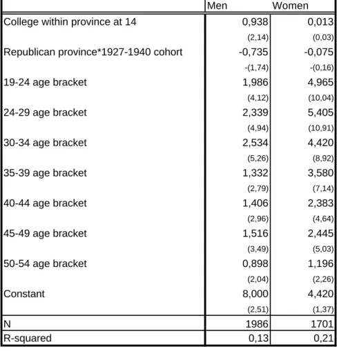
Table 1 presents the estimates for the years of schooling function that we use to form the prediction to be included as a regressor in the wage equation in our IV estimator. The default worker is aged over 54, resided in a province without a college at
the age of 14 and this province adhered to the military rebellion.14 Note that the
availability of a college within the province of residence at 14 has a positive and significant effect in the case of men but not in the case of women. Concerning the age profiles note that, in both genders, those born before 1936 are the least schooled. However, in the case of men born before 1940, to have resided in a republican province is associated to nearly one year less of schooling than the rest of men in the same cohort (the effect is significant at the 9% level). This suggests that the educational choices of men and women have followed different patterns. In particular, note that the differences in average schooling between men and women widen as we look at older cohorts, reflecting the fact that the equal proportion of genders in nowadays classes is a relatively recent phenomenon in Spain. It is therefore not surprising that the existence of a college in the province or the differential effect of the war on old cohorts only affected men. Thus the pace of the increase in schooling acquisition along cohorts is more rapid for women. For instance, while there are no significant differences in the levels of schooling between men born in the late fifties and men born in the mid sixties (the 24-29 and
34 age brackets respectively), the difference in the expected schooling level of women in these two cohorts is around one year.
The residual from these regressions is included in the wage equation in order to
perform an exogeneity test on education,15 obtaining a significant t-value for both men
and women, which confirms the presumed endogeneity of schooling.
Insert table 1 about here
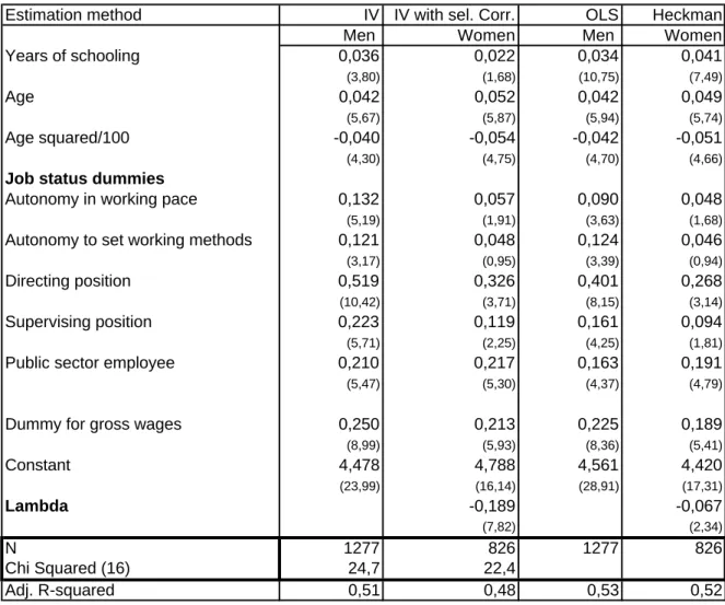
In table 2 we present the OLS and IV estimates (selectivity corrected in the case
of women)16 for the wage equation and the chi squared statistic for a Hausman
exogeneity test on the job status and sectoral dummies included in the specification. Although the primary concern of the paper is not the estimated effects at the mean, it is useful to discuss these results for they provide a benchmark against which the quantile regression estimates might be compared. Also, they are useful to indicate in which direction operates the bias induced by the endogeneity/measurement error of education. In fact, note that the results obtained treating education as an exogenous variable generate a greater return to a year of schooling for women and a lower one for men. When education is instrumented the return to a year of schooling for men increase slightly (from 3.4% to 3.6%). However, the returns to schooling shrink by one half for women when the former is instrumented. The direction of the bias in the case of males
is in accordance with the majority of the results reported in the literature using samples
of male workers,17 which suggest that OLS are biased downwards due to measurement
error in schooling. In contrast, the shrink in the estimate for the returns to schooling in the population of women is less common. Indeed, Butcher and Case (1993) report a downward bias in OLS estimations, much in the same fashion as the results using male samples. However, there are precedents for this result in the literature, as Neumark and Korenman (1994) detect an upward bias in OLS estimates when they treat schooling as an endogenous variable using a sample of females. A potential explanation for this result is that in the case of Spanish women, the contribution of measurement error to the bias is low in comparison with the contribution of the effect of unobserved intellectual abilities correlated with years of education, which render OLS upwardly biased. In view of the differential pattern of education followed by men and women in the last decades in Spain (table 1), it is reasonable to expect that the mechanism that selects the more intellectually able individuals into education has operated with more strength in the case of women than men.
The returns to education seem to be low in comparison to the reported estimates in other studies for Spanish workers. For instance, using data from 1990 for a sample of
wage earners, Alba-Ramírez and San Segundo (1995) report a return per year of 7.3%
for males and 9.8% for females. In order to check for the consistency of our results, we estimate a wage equation by OLS using the same specification as these authors: a
16 We have not found evidence of selectivity problems for the male sample. In the probit equation for
labour market participation we include age, marital status, number of income earners at the household, a set of educational attainment dummies for the worker and his/her mother and a set of regional dummies.
constant, a proxy for experience and its square and years of education (treated as an exogenous variable), and we obtain estimates of 7.3% for males and 9% for females. Therefore the apparently small size of our estimates would seem to be due to a fuller specification of the wage equation.
Turning now to the effects of the job status dummies, and focusing on the IV estimates, note that while the coefficients on the autonomy to set working pace and methods autonomy indicators suggest, respectively, a wage premium of 5% and 4% in the case of women, the male counterparts are large and significant, with an associated
reward of 13% and 12% respectively with respect to the default category.18 The returns
associated to the directing and supervising positions are greater for men, 51% and 22% respectively, than for women, 32% and 11%. The reward for public employees at the mean of the conditional wage distribution is roughly equivalent for women (21,7%) and
men (21%).19
Insert table 2 about here
4.2 Quantiles of the conditional wage distribution
Tables 3 and 4 present the estimates for the conditional quantile functions using the same specification as that of the conditional mean, treating education as an
17 See Card (1994) and Harmon and Walker (1996, 1997). 18
The associated coefficient for autonomy in setting working methods is not significantly different from zero however.
19
The differences in public and private sector wages in Spain have been analysed by García et al. (1997) using quantile regression techniques.
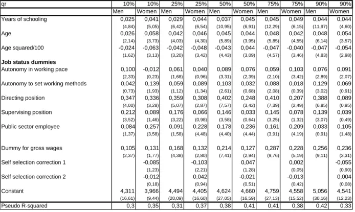
exogenous or endogenous variable respectively. The selectivity correction for the women’s wage equation has been carried out along the lines discussed in Buchinsky (1996). First, we obtain an estimate of the latent index that determines labour market participation through a standard probit. Then, we use it as the argument in a power series expansion that approximates the unknown quantile functions of the truncated
bivariate distribution for the error terms in the wage and the participation equations.20
The covariance matrix for the two stage quantile regression and the selectivity corrected estimates is obtained by bootstrapping the design matrix with 100 replications, while the covariance matrix for the standard quantile regression estimates in the male wage equation is based on the Koenker and Basset (1978) algorithms.
Insert tables 3 and 4 about here
The pattern of differences in the direction of the OLS bias in the estimates for the returns to education that we have at the conditional mean is generally preserved along the conditional quantiles for both men and women, although in some instances the loss of precision is big enough to render some coefficients not significant in the case of women. The two stage LAD estimates for male workers are greater than the LAD counterparts up to the conditional median and third quartile. However, at the ninth decile the two-stage LAD estimate is 3.1% while the uncorrected one is 4.4%. In the case of women, the corrected estimate is always below the uncorrected one.
20
Of the alternatives suggested by Buchinsky we use the one based in the inverse Mill’s ratio with three terms.
Concerning the change in the contribution of schooling to the quantiles as we move along the distribution, note that while the returns to schooling rise from 3% at the bottom decile up to 4.5% at the third quartile of the male conditional wage distribution, they are bounded by 2.9% (third quartile) in the case of women. This suggests that
education is a relatively weak source of overall wage dispersion in Spain.21
Nevertheless, education contributes to generate wage differentials among genders. Moreover, these results suggest that increasing the overall level of education in the population would not help to reduce gender inequality. The reason is that more years of schooling would make male wages more disperse whereas female wages would not experience a significative increase in dispersion.
When we focus on the estimates for the job status indicators in table 4, we detect, on the one hand, that the gap between estimates for the autonomy in setting the working pace dummy narrows as we move up the pay scale. On the other hand there is no clear pattern in the estimates for the autonomy in setting working methods dummy. It should be noted that these two indicators have a subjective nature and consequently there is not much information to be extracted from their associated coefficients as far contribution to overall wage inequality and gender inequality is concerned. However, they act as controls for unobserved job characteristics and their effect is significant at several points of the distribution so there is a clear case for their inclusion in the specification. The director, supervisor and public employee indicators are, on the contrary, objective job characteristics and, moreover, their associated coefficients reveal
21
The results for Portugal in 1995 reported by Machado and Mata (1999) range from more than 5% at the second decile to more than 10% in the 8th decile.
interesting information for the causes of gender inequality and its changing size over the wage scale. Firstly note that the gender gap between the rewards associated to occupying a directing position widens as we move up in the conditional wage distribution: 8% in the first decile and 47% in the ninth decile. Secondly, the same pattern is found in the coefficients for the supervisor dummy: 6% in the first decile and 13% in the ninth decile. This suggests that even if women had access to promotions to supervisor and director posts at the same pace as men, gender inequality would increase because the induced spread in the wage density would be greater for men than women. When we inspect the coefficients for the public employee dummy, we find quite the opposite pattern. The returns are greater for women but the gap narrows as we move up the pay scale. Note also that the size of the coefficients for both genders decreases as we move up the pay scale. This suggests that, as expected, public employment tends to reduce overall wage inequality and also gender wage inequality.
According to these results, the sources of gender wage inequality among Spanish workers appear not to reside in differential returns to education but in sizeable asymmetries in the rewards to job status.
Finally, we find that the coefficient of the first correction term for sample selection is significant and negative in all the quantiles. However, its contribution to wage dispersion among employed women is not clear, although the value of the parameters displays an inverted U shape throughout the distribution.
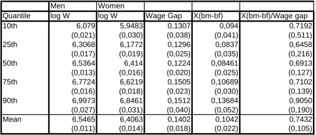
The following table presents the predicted mean and the predicted 10th, 25th, 50th, 75th and 90th quantiles of the log wage distribution conditioned on the vector of
mean characteristics in the sample.22 The table also includes the gender wage gap
calculated from these estimates and the part of the latter that can be attributed to
different returns to the same characteristics.23 For all these measures we also report
bootstrapped standard errors. For comparison, we also report the observed quantiles of the (marginal) wage densities in the data appendix.
Insert table 5 here
Note that the predicted mean and all quantiles are always greater for men than for women. Also, the wage gap that the model estimates predict for workers with the mean sample characteristics is greater at high salaries. In particular, the greatest difference is found at the ninth quartile (15.12%), followed closely by the gap at the third quartile (15.05%). Note, however, that in relation to the absolute wage gap, the “unexplained by observable characteristics” wage difference is much greater at top salaries, reaching 90.5% at the ninth decile. It seems clear that the results that we obtain from the conditional mean estimates, which would suggest that three quarters of the wage gap are due to different returns to characteristics, fail to represent accurately the pattern of differences encountered along the distribution. Unfortunately, the precision of
22 We have experimented with alternative vectors of characteristics and the results do not change
substantially.
23 We follow Neuman and Oaxaca (1998) and consider differences in the coefficient for the selection term
(zero in the case of males) as manifestations of discrimination. In this sense, the female selectivity correction term is included in the part of the wage gap due to discrimination in our decomposition.
these estimates is not very high so the implications we are about to discuss do not have a conclusive nature. It is clear, therefore, that further research should be devoted to establish whether the differences detected with the point estimates are statistically significant. However, the sign and size of the patterns we have found in the latter suggest some interesting implications for the methodology of wage gap measurement.
Indeed, the main stylised fact emerging from our results relates to the measure of discrimination we have defined in section 2. Recall that the main conceptual issue behind expression (4) resides in the fact that perceptions of wage discrimination by an individual worker are based on a richer set of information than that at the disposal of the econometrician. In this sense the relevant wage gap for a potentially discriminated worker is the wage that separates her from another worker with not only the same observed characteristics but also the same unobserved characteristics. The econometrician can approach this wage gap by first identifying which quantile in the wage distribution (conditional on the worker’s observed characteristics) does the worker situate upon, and then measuring the difference up to the predicted equivalent quantile of the wage density for the other group (conditioning on the same set of characteristics). Finally, this wage gap can be decomposed as usual into the discriminatory and non-discriminatory components. In the case of differences between male and female wage schedules in Spain, we find that this procedure yields not only different absolute wage gaps according to the location of the worker in the distribution of wages, but also that the weight of differential returns to characteristics between the two groups changes depending on such location.
Moreover, the pattern of unequal gaps between male and female wages is such that both their absolute size and the portion that can be attributed to discrimination increase over the pay scale. This pattern could provide an explanation to the lack of a clear relationship between traditional, conditional mean based, measures of discrimination and the tendency to report being discriminated against on behalf of women which Kuhn (1987) and Hallock et al. (1998) report. Our proposed explanation is that the measures used by these authors might fail to proxy adequately perceived wage discrimination. Also, it is tempting to suggest that the measure we define in this paper might capture individual perceptions more closely. Unfortunately, we cannot provide a formal statistical test for such claim since we lack information on individual perceptions for the women in our sample. However, note that Kuhn reported a significant and positive effect of the salary level on the probability of reporting discrimination and, remarkably, our measure of discrimination increases with wages too. An issue of interest in the research agenda within the area of gender discrimination would consist in checking whether this pattern is present in other labour markets, and also whether the measures of discrimination based on quantile regression can explain the probability that a female worker reports discrimination. If a stable link between these new measures and subjective perceptions was to be confirmed, the standard toolbox of statistical measures used in discrimination cases at courtrooms could be improved.
6. Summary
The main motivation of this paper is to re-examine the link between subjective perceptions of discrimination and objective measures that are calculated using estimates from a wage equation. In order to do so we have used data on a sample of Spanish
workers to estimate the conditional mean and quantiles of the wage distribution of men and women with a view to quantifying and decomposing their differences into the part attributable to different characteristics and the part attributable to different returns to the same characteristics. In the estimation exercise we take into account the potential endogeneity of education and the usual selectivity problem in wage equations for females.
Our results suggest that the wage gap increases with the pay scale: while the wage floor of the best paid 50% of men with average characteristics is estimated to be around 12% greater than the wage floor of the best paid 50% of women, the wage floor for the best paid 10% of men is around 15% greater than that of the best paid 10% of women. Moreover, the decomposition of the wage gap in the spirit of the Oaxaca (1973) methodology reveals that the “unexplained part” is greater both in absolute terms and relative terms as we move up along the wage scale: while different returns generate a wage differential of roughly 8% at the first quartile of the conditional wage distribution and this accounts for two thirds of the full gap, at the ninth decile different returns generate a difference of more than 13 percentage points, which account for 90% of the full gap. Even if it is not possible to test formally whether such differentials are caused by discrimination or unobserved differences in productivity, the results are consistent with the reported claims of more frequent and greater discrimination on behalf of women at high salary levels. Therefore, given the nature of the data usually available, an attractive way of proxying subjective perceptions is to use decompositions based on quantile regression estimates.
Our results also provide evidence on the underlying sources of wage dispersion in Spain, which seem to be related to job characteristics, rather than worker characteristics such as education.
References
Abadie, A. (1997). “Changes in the Spanish Labour Income Structure During the 1980’s: a Quantile Regression Approach”. Investigaciones Económicas, 21, pp. 253-272.
Alba-Ramírez, A. and M.J. San Segundo (1995). “The Returns to Education in Spain”. Economics of Education Review, 14, pp. 155-166.
Amemiya, T. (1982). “Two-Stage Least Absolute Deviations Estimators”. Econometrica, 50, pp. 689-711.
Angrist, J. and A. Krueger (1991). “Does Compulsory Schooling Attendance Affect Schooling and Earnings?”. The Quarterly Journal of Economics, 106, pp. 979-1014. Barbezat, D. and J. Hughes (1990). “Sex Discrimination in Labor Markets: The Role of Statistical Evidence: Comment.” American Economic Review, 80 pp. 277-286.
Blau, F. and L. Kahn (1992). “The Gender Earnings Gap: Learning from International Comparison.” American Economic Review, 82, pp. 533-538.
Blau, F. and L. Kahn (1997). “Swimming Upstream: Trends in the Gender Wage Differential in the 1980s.” Journal of Labor Economics, 15, pp. 1-42.
Blinder, A. S. (1973) “Wage Discrimination: Reduced Form and Structural Estimates”, The Journal of Human Resources, 8, pp. 436-455.
Buchinsky, M. (1994). “Changes in the U.S. Wage Structure 1963-1987: Application of Quantile Regression”. Econometrica, 62. pp. 405-458.
Buchinsky, M. (1996). “Women’s Return to Education in the US. Exploration by Quantile Regression with Non- Parametric Sample Selection Correction”. Working Paper. Department of Economics. Brown University.
Buchinsky, M. (1997). “Recent Advances in Quantile Regression Models: A practical Guideline for Empirical Research”. Forthcoming in The Journal of Human Resources. Butcher, K. and A. Case (1994). “The Effect of Sibling Composition on Women’s Education and Earnings”. The Quarterly Journal of Economics, 109,3, pp. 531-563. Callan, T. and A. Wren (1994). “Male-Female Wage Differentials: Analysis and Policy Issues”: The Economic and Social Research Institute. General Research Series Paper 163. Dublin.
Card, D. (1994). “Earnings, Schooling and Ability Revisited”. National Bureau of Economic Research. Working Paper no. 4832.
Chamberlain, G. (1994). “Quantile Regression, Censoring and the Structure of Wages” in C.A. Sims, eds. Advances in Econometrics 6th World Congress. Vol 1. Cambridge University Press.
Choudury, S. (1994). “Reassessing the Male-Female Wage Differential: A Fixed Effects Approach.” Southern Economic Journal, 60, pp. 327-324.
De la Rica, S. and A. Ugidos (1995). “¿Son las Diferencias en Capital Humano Determinantes de las Diferencias Salariales Observadas entre Hombres y Mujeres?”. Investigaciones Económicas, 19, pp. 395-414.
Di Nardo, J. Fortin, N. and Lemieux, T. (1996). “Labor Market Institutions and the Distribution of Wages, 1973-1992: A Semiparametric Approach”. Econometrica, 64, pp. 1001-1044.
Even W. (1990) “Sex Discrimination in Labor Markets: The Role of Statistical Evidence:Comment.” American Economic Review, 80, pp. 287-289.
Fortin, N. and T. Lemieux (1998). “Rank Regressions, Wage Distributions, and the Gender Gap”. Journal of Human Resources, 33, pp. 610-643.
García, J., P.J. Hernández and A. López (1997). “Diferencias Salariales entre Sector Público y Sector Privado en España”. Papeles de Economía Española, 72, pp. 261-274. Hallock, K.F. W. Hendricks and E. Broadbent (1998). “Discrimination by Gender and Disability Status: Do Workers Perceptions Match Statistical Measures?”. Southern Economic Journal, 65, pp. 245-263.
Harkness, S. (1996). “The Gender Earnings Gap: Evidence from the UK”. Fiscal Studies, 17, pp. 1-36.
Harmon, C. and I. Walker (1995). “Estimates of the Economic Return to Schooling for the United Kingdom”. American Economic Review, 8, pp. 1279-1286.
Harmon, C. and I. Walker (1996). “The Marginal and Average Returns to Schooling”. Institute for Fiscal Studies Working Paper 96/11. London.
Hernández, P.J. (1995). “Análisis Empírico de la Discriminación Salarial de la Mujer en España”. Investigaciones Económicas, 19, pp. 195-215.
Hernández, P.J. (1996). “Segregación Ocupacional de la Mujer y Movilidad Laboral”. Revista de Economía Aplicada, 4, pp. 57-80.
Hernández, P.J. (1997). “Causas y Consecuencias del Abandono Voluntario del Puesto de Trabajo en la Mujer”. Cuadernos Económicos del ICE, 63, pp. 125-154.
Juhn, C., K. Murphy, and B. Pierce (1993). “Wage Inequality and the Rise in the Returns to Skill”. Journal of Political Economy, 101, pp. 410-442.
Kim, M. and S. Polachek (1994). “Panel Estimates of Male-Female Earnings Functions.” The Journal of Human Resources, 29, pp. 407-427.
Koenker, R. and G. Bassett (1978). “Regression Quantiles”. Econometrica, 46, pp. 33-50.
Kuhn, P. (1987). “Sex Discrimination in Labor Markets: The Role of Statistical Evidence”. American Economic Review, 77, pp. 567-583.
Kuhn, P. (1990). “Sex Discrimination in Labor Markets: The Role of Statistical Evidence: Reply”. American Economic Review, 80, pp. 290-297.
Machado, J.A.F. and Mata, J. (1999). “Sources of Increased Wage Inequality”. Mimeo. Mueller, R. (1998), “Public-Private Sector Wage Differentials in Canada: Evidence from Quantile Regression”. Economics Letters, 60, pp. 229-235.
Neuman, S. and R. Oaxaca (1998). “Estimating Labor Market Discrimination with Selectivity Corrected Wage Equations: Methodological Considerations and An Illustration from Israel”. Center for Economic Policy Research. Discussion Paper 1915. Neumark, D. (1988). “Employers Discriminatory Behaviour and the Estimation of Wage Discrimination”. The Journal of Human Resources, 23, pp. 279-295.
Neumark, D. and S. Korenman (1994). “Sources of Bias in Women’s Wage Equations: Results Using Siblings Data.” The Journal of Human Resources, 29, pp. 378-485.
Oaxaca, R. (1973). “Male-Female Wage Differentials in Urban Labour Markets.” International Economic Review, 14. pp. 693-709.
Powell, J. (1983). “The Asymptotic Normality of the Two Stage Least Absolute Deviations Estimator.” Econometrica, 51, 1569-1575.
Poterba, J. and K. Rueben (1994). “The Distribution of Public Sector Wage Premia: Evidence Using Quantile regression Methods”. National Bureau of Economic Research W.P. 4734.
Prieto, J. (1995). “Discriminación Salarial por Sexos y Movilidad Laboral”. Ph. D. Thesis. Universidad de Oviedo.
Ribeiro, E. (1997). “Conditional Labour Supply Quantile Estimates in Brazil”. Texto Para Discussao no. 97/02. Universidade Federal do Rio Grande do Sul.
Rutemiller, H. C. and D. A. Bowers (1968). “Estimation in a Heteroskedastic Regression Model.” Journal of the American Statistical Association, 63, pp. 552-557. Smith R. and R. Blundell (1986). “An Exogeneity Test for a Simultaneous Equation Tobit Model with an Application to Labour Supply”. Econometrica, 54, pp. 679-685. Thomas, H. (1965). The Spanish Civil War, Hardmondworth Penguin. London.
Ugidos, A. (1993). “Gender Wage Differences and Sample Selection: Evidence from Spain”. Paper presented at the XVIII Simposio de Análisis Económico. Barcelona. Ullibarri, M. (1996). “La Discriminación Salarial por Sexo y la Segmentación Ocupacional en España: un Análisis Desagregado”. Ph. D. Thesis. Universidad Pública de Navarra.
Wright, R. and J. Ermisch (1991). “Gender Discrimination in the British Labour Market: A Reassessment”. Economic Journal, 101, pp. 508-522.
Abstract
In this paper we re-examine the link between subjective perceptions and objective measures of wage discrimination by estimating the mean and several quantiles in the conditional wage distribution of men and women in order to decompose the gender wage gap into the part attributed to different characteristics and the part attributable to differential returns to these characteristics at points other than the conditional expectation. In the process we take into account the endogeneity of educational choice and the participation decision of women. The results suggest that the absolute wage gap and the component of the latter that can be attributed to different returns to characteristics increase over the wage scale.
Table 1. Auxiliary education equation estimates
Men Women
College within province at 14 0,938 0,013
(2,14) (0,03)
Republican province*1927-1940 cohort -0,735 -0,075
-(1,74) -(0,16) 19-24 age bracket 1,986 4,965 (4,12) (10,04) 24-29 age bracket 2,339 5,405 (4,94) (10,91) 30-34 age bracket 2,534 4,420 (5,26) (8,92) 35-39 age bracket 1,332 3,580 (2,79) (7,14) 40-44 age bracket 1,406 2,383 (2,96) (4,64) 45-49 age bracket 1,516 2,445 (3,49) (5,03) 50-54 age bracket 0,898 1,196 (2,04) (2,26) Constant 8,000 4,420 (2,51) (1,37) N 1986 1701 R-squared 0,13 0,21
Table 2. Estimates for the conditional mean of the wage distribution. OLS and IV with selectivity correction. Absolute value of t-statistics in parenthesis
Estimation method IV IV with sel. Corr. OLS Heckman
Men Women Men Women
Years of schooling 0,036 0,022 0,034 0,041 (3,80) (1,68) (10,75) (7,49) Age 0,042 0,052 0,042 0,049 (5,67) (5,87) (5,94) (5,74) Age squared/100 -0,040 -0,054 -0,042 -0,051 (4,30) (4,75) (4,70) (4,66)
Job status dummies
Autonomy in working pace 0,132 0,057 0,090 0,048
(5,19) (1,91) (3,63) (1,68)
Autonomy to set working methods 0,121 0,048 0,124 0,046
(3,17) (0,95) (3,39) (0,94)
Directing position 0,519 0,326 0,401 0,268
(10,42) (3,71) (8,15) (3,14)
Supervising position 0,223 0,119 0,161 0,094
(5,71) (2,25) (4,25) (1,81)
Public sector employee 0,210 0,217 0,163 0,191
(5,47) (5,30) (4,37) (4,79)
Dummy for gross wages 0,250 0,213 0,225 0,189
(8,99) (5,93) (8,36) (5,41) Constant 4,478 4,788 4,561 4,420 (23,99) (16,14) (28,91) (17,31) Lambda -0,189 -0,067 (7,82) (2,34) N 1277 826 1277 826 Chi Squared (16) 24,7 22,4 Adj. R-squared 0,51 0,48 0,53 0,52
Table 3. Quantile regression estimates corrected for selectivity. Absolute value of t-statistics in parenthesis.
qr 10% 10% 25% 25% 50% 50% 75% 75% 90% 90%
Men Women Men Women Men Women Men Women Men Women Years of schooling 0,025 0,041 0,029 0,044 0,037 0,045 0,045 0,049 0,044 0,044 (4,84) (5,05) (6,42) (6,54) (10,95) (6,91) (12,29) (6,15) (11,97) (4,60) Age 0,026 0,058 0,042 0,046 0,045 0,044 0,048 0,042 0,048 0,054 (2,14) (3,73) (4,03) (4,30) (5,89) (3,95) (5,85) (4,55) (6,14) (3,57) Age squared/100 -0,024 -0,063 -0,042 -0,048 -0,043 0,044 -0,047 -0,040 -0,047 -0,054 (1,62) (3,13) (3,20) (3,42) (4,43) (3,09) (4,57) (3,46) (4,83) (2,98) Job status dummies
Autonomy in working pace 0,100 -0,012 0,061 0,040 0,089 0,076 0,059 0,103 0,076 0,091
(2,33) (0,23) (1,68) (0,96) (3,31) (2,39) (2,10) (3,42) (2,89) (2,07)
Autonomy to set working methods 0,042 0,139 0,059 0,089 0,103 0,032 0,088 0,018 0,129 0,069
(0,73) (1,93) (1,12) (1,34) (2,61) (0,68) (2,08) (0,39) (3,02) (0,91)
Directing position 0,347 0,336 0,359 0,308 0,402 0,248 0,410 0,207 0,388 0,089
(4,00) (3,28) (5,07) (2,87) (7,57) (3,42) (7,39) (2,49) (6,85) (0,95)
Supervising position 0,212 0,089 0,176 0,066 0,146 0,033 0,145 0,078 0,139 0,039
(3,52) (1,46) (3,22) (0,98) (3,58) (0,64) (3,25) (1,32) (3,07) (0,49)
Public sector employee 0,084 0,257 0,091 0,228 0,178 0,236 0,161 0,209 0,033 0,105
(1,37) (3,58) (1,58) (4,48) (4,40) (4,44) (3,91) (4,19) (0,91) (1,48)
Dummy for gross wages 0,105 0,131 0,168 0,132 0,214 0,127 0,287 0,228 0,256 0,236
(2,37) (1,77) (4,38) (2,80) (7,41) (2,94) (9,76) (5,19) (9,11) (3,31)
Self selection correction 1 -0,085 -0,103 0,047 0,002 -0,055
(1,23) (2,21) (1,28) (0,05) (0,90)
Self selection correction 2 -0,012 0,042 -0,021 -0,013 0,004
(0,18) (0,94) (0,51) (0,42) (0,08)
Constant 4,311 3,966 4,494 4,405 4,624 4,660 4,759 4,558 5,056 4,541
(16,61) (9,44) (20,09) (16,60) (27,05) (16,59) (27,13) (15,52) (30,16) (12,23)
Pseudo R-squared 0,3 0,35 0,31 0,37 0,38 0,41 0,41 0,38 0,42 0,33 The results for the 11 sectoral dummies and 16 regional dummies are available on request.
Table 4.Two Stage Quantile Regression estimates corrected for selectivity. Absolute value of t-statistics in parenthesis
2sqr 10% 10% 25% 25% 50% 50% 75% 75% 90% 90%
Men Women Men Women Men Women Men Women Men Women Years of schooling 0,030 0,022 0,036 0,026 0,031 0,021 0,045 0,029 0,031 0,021 (1,65) (1,17) (2,77) (1,53) (3,57) (1,24) (4,81) (2,62) (1,64) (0,97) Age 0,038 0,069 0,042 0,052 0,042 0,050 0,035 0,049 0,045 0,047 (2,86) (3,90) (4,79) (4,94) (5,07) (4,39) (4,05) (4,91) (3,15) (3,15) Age squared/100 -0,038 -0,079 -0,041 -0,056 -0,039 -0,052 -0,028 -0,046 -0,044 -0,044 (2,33) (3,53) (3,52) (3,86) (3,64) (3,23) (2,62) (3,74) (2,34) (2,48) Job status dummies
Autonomy in working pace 0,111 0,033 0,091 0,042 0,135 0,063 0,149 0,122 0,121 0,170
(2,62) (0,65) (2,54) (1,05) (4,47) (1,79) (4,43) (3,32) (1,98) (3,46)
Autonomy to set working methods 0,004 0,032 0,058 0,021 0,121 0,022 0,119 0,078 0,104 0,103
(0,07) (0,33) (1,09) (0,33) (2,50) (0,29) (2,10) (1,04) (1,27) (1,09)
Directing position 0,432 0,355 0,501 0,389 0,507 0,327 0,553 0,227 0,576 0,101
(3,59) (2,99) (6,78) (3,16) (6,69) (3,78) (6,25) (2,77) (4,03) (0,76)
Supervising position 0,259 0,195 0,252 0,123 0,227 0,114 0,233 0,101 0,212 0,081
(3,96) (1,89) (5,54) (1,83) (5,35) (1,56) (5,10) (1,44) (2,85) (0,91)
Public sector employee 0,123 0,283 0,168 0,277 0,225 0,270 0,226 0,270 0,162 0,182
(2,25) (3,49) (3,73) (4,19) (5,26) (5,52) (4,56) (4,94) (2,48) (2,28)
Dummy for gross wages 0,120 0,131 0,187 0,123 0,230 0,120 0,287 0,235 0,441 0,375
(2,23) (1,62) (4,95) (2,60) (6,92) (2,43) (6,24) (5,02) (5,47) (4,90)
Self selection correction 1 -0,211 -0,187 -0,160 -0,148 -0,220
(2,84) (3,88) (4,52) (3,36) (5,28)
Self selection correction 2 0,016 -0,027 -0,023 0,024 0,034
(0,21) (0,48) (0,45) (0,64) (0,62)
Constant 3,956 4,385 4,363 4,704 4,660 4,953 4,759 4,869 5,029 5,000
(9,71) (11,03) (18,74) (14,36) (23,30) (18,16) (21,61) (21,42) (16,10) (10,26)
Pseudo R-squared 0,28 0,32 0,29 0,35 0,34 0,39 0,36 0,34 0,36 0,3 The results for the 11 sectoral dummies and 16 regional dummies are available on request.
Table 5. Predicted Wage Gaps and Decomposition. Boostrapped standard errors in parenthesis.
Men Women
Quantile log W log W Wage Gap X(bm-bf) X(bm-bf)/Wage gap 10th 6,079 5,9483 0,1307 0,094 0,7192 (0,021) (0,030) (0,038) (0,041) (0,511) 25th 6,3068 6,1772 0,1296 0,0837 0,6458 (0,017) (0,019) (0,025) (0,035) (0,216) 50th 6,5364 6,414 0,1224 0,08461 0,6913 (0,013) (0,016) (0,020) (0,025) (0,127) 75th 6,7724 6,6219 0,1505 0,10689 0,7102 (0,016) (0,018) (0,023) (0,030) (0,139) 90th 6,9973 6,8461 0,1512 0,13684 0,9050 (0,027) (0,031) (0,040) (0,052) (0,190) Mean 6,5465 6,4063 0,1402 0,1042 0,7432 (0,011) (0,014) (0,018) (0,022) (0,105)
DATA APPENDIX Descritive statistics
Men Women
Mean Stand. Dev. Mean Stand. Dev.
Years of schooling 11,467 4,616 12,412 3,92
Age 37,020 10,876 34,045 10,471
Dummy for gross wages 0,246 0,431 0,203 0,403
Log(wage) 6,546 0,577 6,406 0,556
Job status dummies
Autonomy in working pace 0,407 0,491 0,412 0,492
Autonomy to set working methods 0,236 0,425 0,139 0,346
Directing position 0,096 0,295 0,03 0,171
Supervising position 0,187 0,390 0,121 0,326
Public sector employee 0,349 0,477 0,462 0,499
Number of observations 1277 826
Men Women
Quantile Stand. Dev. Quantile Stand. Dev.
10th 5,927 0,023 5,723 0,033
25th 6,134 0,012 6,001 0,016
50th 6,489 0,03 6,369 0,027
75th 6,888 0,029 6,828 0,022