Munich Personal RePEc Archive
Bayesian dynamic variable selection in
high dimensions
Korobilis, Dimitris and Koop, Gary
University of Glasgow
5 May 2020
Online at
https://mpra.ub.uni-muenchen.de/100164/
Bayesian dynamic variable selection in high dimensions
Gary Koop
University of Strathclyde
Dimitris Korobilis
✯University of Glasgow
AbstractThis paper proposes a variational Bayes algorithm for computationally efficient posterior and predictive inference in time-varying parameter (TVP) models. Within this context we specify a new dynamic variable/model selection strategy for TVP dynamic regression models in the presence of a large number of predictors. This strategy allows for assessing in individual time periods which predictors are relevant (or not) for forecasting the dependent variable. The new algorithm is evaluated numerically using synthetic data and its computational advantages are established. Using macroeconomic data for the US we find that regression models that combine time-varying parameters with the information in many predictors have the potential to improve forecasts of price inflation over a number of alternative forecasting models.
Keywords: dynamic linear model; approximate posterior inference; dynamic variable selection; forecasting
JEL Classification: C11, C13, C52, C53, C61
✯Corresponding Author: Adam Smith Business School, University of Glasgow, G12 8QQ Glasgow, UK,
1
Introduction
Regression models that incorporate stochastic variation in parameters have been used by
economists at least since the work Cooley and Prescott (1976). Thirty years later,Granger
(2008) argued that time-varying parameter models might become the norm in econometric
inference since, as he illustrated via White’s theorem, time variation is able to approximate generic forms of nonlinearity in parameters. Indeed, initiated by the unprecedented shocks observed during and after the Global Recession of 2007-9, a large recent literature has established the importance of modeling time variation in the intercept, slopes and variance
of regressions for forecasting economic time series; see Stock and Watson (2007) for a
representative example of a model using only a stochastic intercept and volatilities. At the same time, the stylized fact that economic predictors are short-lived – that is, relevant for
the dependent variable only in short periods1 – has emerged in various forecasting problems
such as inflation (Koop and Korobilis, 2012), stock returns (Dangl and Halling, 2012) and
exchange rates (Byrne et al., 2018). Following these observations, there is no shortage of
recent econometric work on methods for penalized estimation of time-varying parameter models via classical or Bayesian shrinkage, as well as variable selection methods; see for
example Belmonte et al. (2014), Bitto and Fr¨uhwirth-Schnatter (2019), Kalli and Griffin
(2014), Callot and Kristensen (2014), Korobilis (2019), Kowal et al. (2019), Nakajima and
West (2013), Roˇckov´a and McAlinn (2017), Uribe and Lopes (2017) and Yousuf and Ng
(2019).
In this paper we add to this literature by proposing a new dynamic variable selection prior and a novel, for the field of economics, Bayesian estimation methodology. In particular, we propose to use variational Bayes (VB) inference to estimate time-varying parameter regressions using state-space methods. Variational inference has long been used in data science problems such as large-scale document analysis, computational neuroscience, and computer vision (Blei et al., 2017). Nevertheless, it is only relatively recently that posterior consistency and other theoretical properties of these methods have been explored by
mainstream statisticians (Wang and Blei,2019). Variational inference is a unified estimation
methodology which shares similarities with the Gibbs sampler that many economists
traditionally use to estimate time-varying parameter models (see for example Stock and
Watson, 2007). Like the Gibbs sampler, parameter updates are derived for one parameter
at a time conditional on all other parameters using an iterative scheme. Unlike the Gibbs sampler, there is no repeated sampling involved and the output of VB is typically the first
1An alternative terminology for such periods, which is due to Farmer et al. (2018), is “pockets of
two moments of the posterior distribution of parameters. Our first task is to introduce this estimation scheme in the context of TVP regressions, and contrast it to existing estimation algorithms used in economics for capturing structural change.
Our second contribution lies on the development of a dynamic variable selection prior that
is a conceptually straightforward extension of the static variable selection prior of George
and McCulloch (1993). The dynamic extension of this prior allows to tackle the non-trivial
econometric problem of allowing some predictor variables to enter the TVP regression, model
only in some periods of the full estimation sample. With p predictors and T time periods,
dynamic variable selection involves choosing the “best” among 2p models at each point in
time t, for t= 1, ..., T. Such procedure is in line with strong, recent empirical evidence that
different factors might be driving predictability of economic variables over time; see Rossi
(2013) for a thorough review of this idea. By specifying our new prior within a variational
Bayes framework, we are able to derive an algorithm that is numerically stable and can be
extended to much larger pand T than was possible before.2
We show, via a Monte Carlo exercise and an empirical application, that our proposed algorithm works well in high-dimensional, sparse, time-varying parameter settings. Using artificial data we establish that the new algorithm is precise in estimation and in dynamic variable selection, even in settings with more predictors than time-series observations. In a forecasting exercise of various measures of price inflation, we illustrate that our methodology applied to a time-varying parameter regression with 400+ predictors is able to beat a wide range of linear and nonlinear forecasting regressions. The empirical results provide strong evidence that the new algorithm can achieve estimation accuracy comparable to Markov chain Monte Carlo algorithms, while being much faster to run. The additional feature of dynamic variable selection successfully prevents overparametrization, since our high-dimensional TVP specification is able to beat both parsimonious time series models with no predictors as well as factor models and penalized likelihood estimators.
The remainder of the paper proceeds as follows. Section 2 introduces the basic principles of VB inference for approximating intractable posteriors, and applies these principles to the problem of estimating a simplified time-varying parameter regression model. Section 3 introduces the the novel modelling assumptions, namely dynamic variable selection and stochastic volatility, and derives an estimation algorithm within the VB framework. Section 4 assesses the new algorithm on simulated data. In Section 5 we apply the new methodology to the problem of forecasting US inflation using time-varying parameter regressions with many predictors.
2In particular, many of the algorithms cited above, such asKoop and Korobilis (2012),Kalli and Griffin
2
Variational Bayes inference in state-space models
as variational Bayes (VB) is not an established estimation methodology in econometrics, we first provide a generic discussion of VB methods in approximating intractable posterior distributions. We then apply the generic concepts and formulas to the specific problem of estimating a simplified time-varying parameter regression model with known measurement
error variance.3 Detailed reviews of variational Bayes can be found in Blei et al. (2017) and
Ormerod and Wand (2010), among several others. Variational Bayes estimation of
state-space models is described in detail in the monograph ofSm´ıdl and Quinnˇ (2006), as well as
research papers such as Beal and Ghahramani (2003), Tran et al. (2017), and Wang et al.
(2016).
2.1
Basics of variational Bayes
Consider datay, latent variablessand (latent) parametersθ. Our interest lies in time-varying
parameter models that admit a state-space form. Hence, s represents unobserved state
variables, such as time-varying regression coefficients and time-varying measurement error
variances, and θ represents all other parameters, such as the error covariances in the state
equation. The joint posterior of interest isp(s, θ|y) with associated marginal likelihoodp(y)
and joint density of data and parameters p(y, s, θ). When the joint posterior is complex and
computationally intractable, we can define an approximating density q(s, θ|y) that belongs
to a family F of simpler distributions defined over the parameter space spanned by s, θ.
The main idea behind variational Bayes inference is to make this approximating posterior distributionq(s, θ|y) as close as possible to p(s, θ|y), where “distance” is measured with the
Kullback-Leibler divergence4 KL(q||p) = Z q(s, θ|y) log q(s, θ|y) p(s, θ|y) dsdθ. (1)
That is, the aim is to find the optimal q⋆(s, θ|y) that solves
q⋆(s, θ|y) = arg min
q(s,θ|y)∈F
KL(q||p). (2)
Insight for why KL(q||p) is a desirable distance metric arises from a simple re-arrangement
involving the log of the marginal likelihood (Ormerod and Wand, 2010, page 142) where it
3Readers already familiar with these concepts can skim through this section, and focus on our novel
methodology that is described in the following section
can be shown that logp(y) = logp(y) Z p(s, θ|y) dsdθ = Z p(s, θ|y) logp(y) dsdθ (3) = Z q(s, θ|y) log p(y, s, θ)/q(s, θ|y) p(s, θ|y)/q(s, θ|y) dsdθ (4) = Z q(s, θ|y) log p(y, s, θ) q(s, θ|y) dsdθ+KL(q||p). (5)
BecauseKL(q||p) is non-negative (it is exactly zero whenq(s, θ|y) = p(s, θ|y)), the quantity
G(q(s, θ|y)) = exp Z q(s, θ|y) log p(y, s, θ) q(s, θ|y) dsdθ
≡expEq(s,θ|y)(log (p(y, s, θ))−log (q(s, θ|y)))
,
(6)
becomes a lower bound for the marginal likelihoodp(y).5 The function G(q(s, θ|y)) is known as the Evidence Lower Bound (ELBO). Therefore, instead of minimizing the objective
function KL(q||p) (which cannot be evaluated) we can find an approximating density
q⋆(s, θ|y) that maximizes the marginal data density p(y) by maximizing the ELBO. We
emphasize that Gis a functional on the distributionq(s, θ|y). As a result, the ELBO can be
maximized iteratively using calculus of variations.
If we assume for simplicity the so-called (in Physics) mean field factorization of the form
q(s, θ|y) = q(θ|y)q(s|y), it can be shown6 that the optimal choices for q(s|y) and q(θ|y) are q(s|y) ∝ exp Z q(θ|y) logp(s|y, θ) dθ ≡expEq(θ|y)(logp(s|y, θ)) , (7) q(θ|y) ∝ exp Z q(s|y) logp(θ|y, s) ds ≡expEq(s|y)(logp(θ|y, s)) . (8)
The first expression denotes the expectation over q(θ|y) of the conditional posterior for s,
and the second expression denotes the expectation over q(s|y) of the conditional posterior
for θ. Because q(θ|y) is a function of q(s|y), and vice-versa, the above quantities can be approximated iteratively instead of relying on more computationally expensive numerical
optimization techniques. Given an initial guess regarding the values of (θ, s), VB algorithms
iterate over these two quantities until G(q(s, θ|y)) has reached a maximum. Due to
similarities with the Expectation-Maximization (EM) algorithm of Dempster et al. (1977),
this iterative procedure in its general form is sometimes referred to as the Variational
Bayesian EM (VB-EM) algorithm; seeBeal and Ghahramani(2003). It is also worth noting
5In the following we denote asE
q(•)the expectation w.r.t to a functionq(•).
6A formal and thorough derivation of these ideas is given in the excellent monograph ofˇSm´ıdl and Quinn
the relationship with Gibbs sampling. Like Gibbs sampling, equations (7) and (8) involve the full conditional posterior distributions. But unlike Gibbs sampling, the VB-EM algorithm does not repeatedly simulate from them and is computationally much faster.
2.2
VB estimation of a simple TVP regression model
Before collecting all building blocks of our proposed methodology, we outline a VB algorithm
for the univariate TVP regression with known measurement error varianceσ2. This simplified
model is of the form
yt = xtβt+εt (9)
βt = βt−1+ηt (10)
where yt is the timet scalar value of the dependent variable, t= 1, .., T,xt is a 1×pvector
of exogenous predictors and lagged dependent variables,εt∼N(0, σ2),ηt∼N(0,Wt) with
Wt =diag(w1,t, ..., wp,t) ap×pdiagonal matrix7 and wt= [w1,t, ..., wp,t]′ a p×1 vector. In
likelihood-based analysis of state-space models it simplifies inference if it is assumed thatεt
and ηt are independent of one another and we do adopt this assumption here. Finally, we
use a notational convention where j, t subscripts denote the jth element of a time varying
state variable, or parameter, observed only at time t, while 1 : t subscripts denote all the
observations of a state variable from period 1 up to period t.
The model in equations (9) and (10) has unknown parameters (β1:T,w1:T). Following
the analysis of the previous subsection we first consider the independent prior on the initial conditions β0,w0 of the form
p(β0,w0) = p(β0) p Y j=1 p(wj,0) =N(m0,P0)× p Y j=1 [Gamma(cj,0, dj,0)]−1, (11)
wherewj,0 is the jth element ofw0, andGamma(a, b) denotes the Gamma distribution with
shape parameter a and rate parameter b, that is, the definition of the Gamma distribution
that has meana/b and variancea/b2. The timetprior, conditional on observing information
7By restrictingW
tnot to be a full covariance matrix, coefficientsβitandβjtare uncorrelated a-posteriori
for i 6= j, which might not seem like an empirically relevant assumption. However, allowing for cross-correlation in the state vectorβt can result in counterproductive increases in estimation uncertainty, with
this problem being significantly more pronounced in higher dimensions. A diagonalWt allows for a more
parsimonious econometric specification, less cumbersome derivations of posterior distributions, and faster and numerically stable computation; see alsoBelmonte et al.(2014),Bitto and Fr¨uhwirth-Schnatter(2019) andRoˇckov´a and McAlinn(2017) who adopt a similar assumption.
up to time t−1, is given by the Chapman-Kolmogorov equation p(βt,wt|y1:t−1) = R B,Wp(βt|βt−1) Qp j=1p(wj,t|wj,t−1) × p(βt−1,wt−1|yt−1)dβt−1dw1,t−1...dwp,t−1, (12)
where Bis the support ofβt and Wthe support of allwj,t. Finally, once the measurement
yt is observed, we obtain from Bayes theorem the following timet posterior distribution
p(βt,wt|y1:t)∝p(yt|βt,wt)p(βt,wt|y1:t−1). (13)
This Bayesian joint posterior distribution is rarely analytically tractable, even if conjugate
prior densities have been specified. However, posterior conditionals can be tractable,
and this is why in macroeconomics TVP models are predominantly estimated using the
Gibbs sampler; see Stock and Watson (2007) for an example. Nevertheless, sampling
repeatedly using (Markov chain) Monte Carlo methods is computationally prohibitive in high-dimensional settings or in settings with more flexible likelihood and prior distributions. For that reason we define a tractable variational density as an approximation to the exact intractable time t posterior, that is, we define p(βt,wt|y1:t) ≈ q(βt,wt|y1:t). Among all possible functions q(βt,wt|y1:t) we want to obtain the one that has hyperparameters that
minimize the relative entropy with the true posterior. Following the discussion earlier in this section, this problem is equivalent to maximizing the evidence lower bound (ELBO) of the log-marginal likelihood, that is, it is the solution to
q⋆(βt,wt|y1:t) = arg max q(βt,wt|y1:t) Z q(βt,wt|y1:t) log q(βt,wt|y1:t) p(βt,wt|y1:t) . (14)
This maximization problem is simplified once we assume the mean field factorization of the formq(βt,wt|y1:t) =q(βt|y1:t)
Q
q(wj,t|y1:t) so we can optimizeβtandwtsequentially.
As a result, using variational calculus (ˇSm´ıdl and Quinn, 2006) we can show that the ELBO
is maximized by iterating through the following recursions
q(βt|y1:t) ∝ exp Z logp yt,βt,wt|y1:t−1 Y j q(wj,t|y1:t)dwt ! , (15) q(wj,t|y1:t) ∝ exp Z logp yt,βt,wt|y1:t−1 q(βt|y1:t)dβt , j = 1, ..., p. (16)
Both formulas above become equalities after the addition of a normalizing constant. The first expression is an expectation with respect to the probability density Qjq wj,t|y1:t−1
,
that is, we can write equation (15) using the following form q(βt|y1:t) ∝ exp Eq(wt|y1:t) logp yt,βt,wt|y1:t−1 (17) = exp Eq(wt|y1:t) log p(yt|βt,wt)p βt|y1:t−1 p wt|y1:t−1 (18) = p(yt|βt,wt) exp Eq(wt|y1:t) logp βt|βt−1 + logq βt|y1:t−1 (19)
where q(βt|y1:t−1) is the time t prior of βt obtained from the time t − 1 posterior
q βt−1|y1:t−1 using the Kalman filter recursions, and the term p wt|y1:t−1
in (18)
disappears because the expectation is w.r.t the variational posterior of wt. This latter
representation ofq(βt|y1:t) can be trivially updated by a Normal distribution, with moments
given by the Kalman filter and smoother; see ˇSm´ıdl and Quinn (2006, Chapter 7) for
detailed derivations. We can use similar arguments in order to show that equation (16)
is an expectation that leads to a q w−t1|y1:t of the form G(cj,t, dj,t) (or equivalently to
q(wt|y1:t) that is inverse Gamma).
Algorithm 1Variational Bayes algorithm for TVP regression model with fixed measurement variance
1: Choose values of hyperparametersm0,P0, cj,0, dj,0 forj= 1, ..., p. Setr= 1 and initializeW(r−1).
2: whilekGq(β(r),w(r)|y−Gq(β(r−1),w(r−1)|yk →0do
3: Step 1:Approximate,∀t= 1, ..., T, the posterior
qr (βt|y1:T)∼N(m r t,P r t) conditional onW(r−1) , σ2, wheremr t,P r
t ∀t= 1, ..., T, are obtained using the Kalman filter and the Rauch-Tung-Striebel smoother
4: Step 2:Approximate,∀t= 1, ..., T andj= 1, ..., p, the posterior
qr wj,t−1|y1:T∼G cr j,t, d r j,t conditional onµr t,P r t, wherec r j,t=cj,0+1/2,drj,t=dj,0+Djj,t/2 withDt= Ptr−P r t−1 +m(tr)m(tr)′−mt(r−)1m(t−r)1′. SetW(r)=diagdr 1,t/c r 1,t, ..., d r p,t/c r p,t . 5: r=r+ 1 6: end while
7: Upon convergence set q⋆(β
1:T,w1:T|y1:T) = qr(β1:T|y1:T) × Qpj=1q r
(wj,t|y1:T) using the parameters (mr 1:T,P r 1:T,c r 1:p,1:T,d r
1:p,1:T) obtained during the last iteration of thewhileloop.
Algorithm 1 provides pseudocode for the basic VB estimation problem described in
this section, without assuming either a (dynamic) variable selection prior or stochastic volatility in the measurement equation. In the following section we drop these two unrealistic assumptions.
3
Variational Bayes Inference in High-Dimensional
TVP Regressions
We rewrite for convenience the univariate time-varying parameter model
yt = xtβt+εt (20)
βt = βt−1+ηt (21)
where we define now εt ∼N(0, σ2t) with σ2t a stochastic (time-varying) variance parameter,
and we assume that the dimension p of βt= (β1,t, ..., βp,t)′ is large and possibly p≫T.
3.1
Dynamic variable selection and averaging
The core ingredient of our modeling approach is a dynamic variable/model selection strategy. We specify a dynamic variable selection (DVS) prior that extends the “static” variable
selection prior ofGeorge and McCulloch(1993) that was originally developed for the constant
parameter regression using MCMC and is of the form βj,t|γj,t, τj,t2 ∼ (1−γj,t)N 0, c×τj,t2 +γj,tN 0, τj,t2 , (22) γj,t|πt ∼ Bernoulli(π0,t), (23) 1 τ2 j,t ∼ Gamma(g0, h0) (24) π0,t ∼ Beta(1,1), (25)
for j = 1, ..., p, where c, g0 and h0 are fixed prior hyperparameters. Variable selection
principles require us to setc→0, such that the first component in the prior forβj,tshrinks the
posterior towards zero, while the second component has varianceτ2
j,t which is “large enough”
in order to allow for unrestricted estimation. The choice between the two components in the
prior forβj,t is governed by the random variableγj,t which is distributed Bernoulli and takes
values either zero or one. Ifγj,t = 1 the prior forβj,t has a Normal prior with zero mean and
variance τ2
j,t, while if γj,t = 0 the prior variance becomes cτj,t2 .
Early papers such asGeorge and McCulloch(1993) give very broad guidelines on choosing
values for c and τ2
j,t such that the first component in equation (22) has small enough
variance (to force shrinkage) and the second component has large enough variance (to allow
unrestricted estimation). More recently, Narisetty and He (2014) show that selecting and
fixing the prior variances of such mixture priors could, as T and p grow, lead to model
deterministic functions of the data dimensions T and p. In our case, we do fix c = 10−4
such that the first component has always smaller variance, but we assume τ2
j,t
−1 is a random variable that has a Gamma prior. That way this parameter is always updated by
the information in the data likelihood. The choice of a Gamma prior for τj,t2
−1
implies
that the marginal prior for βj,t is a mixture of leptokurtic Student’s T distributions whose
components could tend to shrink βj,t towards zero, regardless of whether γj,t is zero or
one. Therefore, the proposed prior is able to find patterns of dynamic sparsity as well as impose dynamic shrinkage in time-varying parameters, a property that is very desirable in high-dimensional settings.8
Finally, it becomes apparent that under this variable selection prior setting, bπ0,t =
E(p(π0,t)) = 12 is the time t prior mean probability of inclusion of all predictors in the
TVP regression, while the quantity eπj,t =E(p(γj,t|y1:T)) is the posterior mean probability
of inclusion in the regression of predictorjat time periodt, simply referred to as theposterior inclusion probability (PIP). Due to the fact that all of the hyperparameters γ, π and τ2 are time-varying, our prior allows to obtain time-varying PIPs whose interpretation extends this
of PIPs in constant parameter settings, such as the one inGeorge and McCulloch (1993), in
a straightforward way.
In terms of tackling estimation using this prior we note that adding the prior (22) to our
benchmark TVP specification introduces some peculiarity: by combining equations (10) and
(22) we end up having two conditional prior structures for βj,t, namely
βj,t|βj,t−1, wj,t ∼ N(βj,t−1, wj,t) (26)
βj,t|γj,t, τj,t2 ∼ N(0, vj,t), (27)
where we definevj,t = (1−γj,t)2c×τj,t2 +γj,t2 τj,t2 andVtis thep×pdiagonal matrix comprising
the elements vj,t. Following ideas in Wang et al. (2016) we combine the two priors for βt
described above by rewriting the state equation as9
βt=Fetβt−1+ηet, (28)
8In signal processing a signal (regression coefficient vector) is typically sparse by default, that is, the
researcher knows a-priori to expect that estimates of several coefficients will tend to be exactly zero. In economics, the sparsity assumption might not be empirically founded in certain settings; see the discussion inGiannone et al.(2017). In such cases, a dense model may be preferred, that is, a model where all predictors are relevant with varying weights. While factor models and principal components have been used widely to model dense models in macroeconomics, shrinkage methods are also quite reliable for this task. In particular, we note the result in De Mol et al.(2008) that forecasts from Bayesian shrinkage are highly correlated to forecasts from principal components.
where ηet ∼ N0,Wft, with parameter matrices Wft = E(Wt)−1+E(Vt)−1−1 and e
Ft = Wft×E(Wt)−1, where Wt =diag(w1,t, ..., wp,t) and Vt = diag(v1,t, ..., vp,t), and all
expectation operators are with respect to q(βt|y1:t). Under this formulation we can observe that the joint prior variance forβj,t is a function of bothwj,tandvj,t,∀j = 1, ..., p. Therefore,
the TVP regression model with dynamic variable selection prior can be written using a new
state-space form, with measurement equation given by (9) and state equation given by (28).
Application of algorithm 1 to the transformed state-space model consisting of equations
(20) and (28) provides as output estimates mt|T ∀t, that is, the smoothed posterior
mean of q(βt|y1:T). Conditional on these estimates, derivation of the update steps for
γj,t, τj,t2 and π0,t relies also on deriving the expectations of these variables with respect
to q(βt|y1:T). Therefore, extending the analysis of the previous section to accommodate
these new parameters, and similar to derivations found in Gibbs sampling approaches to
variable selection (see, for instance, the formulas of the conditional posteriors in George and
McCulloch, 1993), the updating steps for the parameters in the dynamic variable selection
prior are the following b τ2 j,t =E q τ2 j,t|yt = h0+m2j,t|T /(g0 + 1/2), (29) b γj,t =E[q(γj,t|yt)] = N mj,t|T|0,bτj,t2 b π0,t N mj,t|T|0,bτj,t2 b π0,t+N mj,t|T|t|0, c×bτj,t2 (1−bπ0,t) , (30) b vj,t =E[q(vj,t|yt)] = (1−bγj,t)2cτbj,t2 +bγj,tbτj,t2 , (31) b π0,t =E[q(π0,t|yt)] = 1 + p X j=1 b γj,t ! /(2 +p), (32)
for each t = 1, .., T and j = 1, ..., p, where again expectations E are with respect to the
VB posteriors of each of the parameters showing up on the right-hand side of the equations above.
q(βt|y1:t−1) to be the timetvariational Bayes prior ofβtgiven information at time t−1. Then we have
q βt|y1:t−1 ∝ expE logp βt|βt−1,Wt +E(logp(βt|Vt)) ∝ exp −1 2 βt−βt−1 ′ W−t1 βt−βt−1 −1 2β ′ tV −1 t βt ∝ exp −1 2β ′ tW−t1βt+βt′W−t1βt−1− 1 2β ′ tV−t1βt ∝ exp −1 2 βt−Fetβt−1 ′ f W−t1 βt−Fetβt−1 ,
where the simplification occurs due to the fact that βt−1 is known and fixed (i.e. not a random variable)
given information at timet−1. Therefore, the formula above specifies the new, joint timetprior ofβtgiven
3.2
Adding stochastic volatility
A known regression variance is far from a realistic assumption for most datasets. When forecasting macroeconomic data, so is the assumption of an unknown variance that is constant over time. A vast recent literature highlights the importance of time-varying
volatility in improving point and density forecasts (Clark and Ravazzolo, 2015), and the
purpose of this subsection is to accommodate estimation of the parameter var(εt) = σt2 in
the VB setting. Several elegant algorithms for VB inference in stochastic volatility models
exist in the literature. For example, Naesseth et al. (2017) introduce a variational Bayes
Sequential Monte Carlo (SMC) algorithm for stochastic volatility models. Tran et al.(2017)
propose a variational Bayes method for intractable likelihoods that does not rely on the mean field approximation, and apply their algorithm to the estimation of a stochastic volatility model.
Nevertheless, such algorithms assume an explicit time-series model for the stochastic volatility parameter, an assumption that is only useful in a setting where one is interested
in forecasting volatility. In a macroeoconomic setting we are interested in forecastingyt and
not its volatility (as it would be the case in empirical asset pricing). At the same time, previous empirical work shows that there are no statistically important differences when
forecasting with alternative specifications of macroeconomic volatility.10 For that reason,
our aim here is not only to render estimation of stochastic volatility precise, but at the same time numerically reliable and computationally efficient. In order to achieve this, we build
on variance discounting ideas for dynamic linear methods as described inWest and Harrison
(1997); see also Roˇckov´a and McAlinn (2017). Defineφt= σ12
t to be the precision (inverse variance). FollowingWest and Harrison(1997)
we assume that the time t−1 posterior ofφ has the following conjugate form
φt−1|y1:t−1 ∼Gamma(at−1, bt−1). (33)
We do not specify an explicit time series model for the dynamics of φ (e.g. stochastic
volatility or GARCH) because the posterior for φt wouldn’t be conjugate to the likelihood
and we would fail to obtain fast updates. In order to maintain this conjugacy we specify
instead the time t prior of the form
φt|y1:t−1 ∼Gamma(δat−1, δbt−1), (34)
10For example, Clark and Ravazzolo (2015) compare a range of specifications for time-varying variance
parameters in univariate and multivariate autoregressive models, and any differences among such specifications are not statistically important (while all volatility specifications are always better relative to constant variance specifications).
for a variance discounting factor 0 < δ < 1, subject to a choice of hyperparameters a0 and
b0. By doing so, we assume thatφtis centered around φt−1 as if this parameter had random
walk dynamics,11 since it holds that E(φ
t|y1:t−1) = E(φt−1|y1:t−1). However, based on the properties of the Gamma distribution, the dispersion of φt is larger to that of φt−1.
Under this scheme the variational Bayes update of φt, that is, its time t posterior mean
has the form
b
φt=Eq(βt|y1:T)(φt|y1:t) = at/bt, (36)
where at = 1/2 +δat−1 and dt = 12
h
yt−xtmt|T)2+xtPt|Tx′t
i
+δbt−1, where mt|T,Pt|T
are the smoothed mean and variance ofβt. Using this scheme, past information in the data is
discounted exponentially by the factorδ. The scalarδcan be seen as a prior hyperparameter
whose choice determines how much relative weight we give to recent versus older observations, that is, it determines how fast we expect the precision parameter to change over time. For
δ= 1 we obtain the posterior under a standard recursive update scheme (similar to recursive
OLS), while typical values that would allow for faster time-variation in the precision/variance would be between 0.8 and 0.99. Values lower than 0.8 are not empirically advised, since they allow for a large amount of time-variation and stochastic variance estimates become very
noisy. In the empirical exercise we set δ = 0.8, a choice that reflects our prior expectation
that macroeconomic data have many abrupt breaks in their second moments and excess kurtosis during recessions (implying variances that can move very fast over time).
The previous formulas pertain to the iterative updating of φt given φt−1. Estimates of
φt can be smoothed using subsequent observationst+ 1, ..., T. Following West and Harrison
(1997) we can run a backward recursive filter of the form
e
φt= (1−δ)φbt+δφet+1, (37)
for t=T −1, ...,1, where φet =Eq(βt|y1:T)(φt|yt+1) andφeT =φbT. Once we obtain this update for the precision φt, a posterior mean estimate of the volatility σt2 can be obtained simply as
the inverse ofφet.
11Even though we haven’t specified an explicit time series evolution forφ
t, by using results inUhlig(1994)
we can show that the proposed variance discounting methodology is equivalent to assuming the following specification:
φt=γtφt−1/δ, (35)
3.3
The Variational Bayes Dynamic Variable Selection (VBDVS)
algorithm
Here we provide details of the exact parameter updates that result from VB inference in
our proposed specification. Algorithm 2 outlines our proposed Variational Bayes Dynamic
Variable Selection (henceforth, VBDVS) algorithm. This Algorithm shows an accurate picture of how this would look like when programmed using a language like MATLAB or R: while there are many parameters involved in our specification, the code is short and it involves simple scalar operations (meaning it is very fast). The only cumbersome operation
is the inversion of the p × p matrix Pt+1|t in line 14 which has worst case complexity
O(p3) for each t. There are four main blocks in this algorithm. Lines 4-12 are a result
of straightforward application of the Kalman filter on the state-space model of equations
(20) and (28), and lines 13-17 show the backwards (smoothing) recursions. Lines 18-27
update the prior hyperparameters of the DVS prior for βt. Finally, lines 28-33 provide
updates for the stochastic volatility parameter, as discussed in the previous subsection.
4
Simulation study
In this section we evaluate the performance of the new estimator using artificial data. Although we view the algorithm as primarily a forecasting algorithm, it is also important to investigate its estimation accuracy in an environment where we know the true data generating process (DGP). Thus, we wish to to establish that the VBDVS is able to track time-varying parameters satisfactorily and establish that the dynamic variable selection prior is able to perform shrinkage and selection with high accuracy (at least in cases where we know that the DGP is that of a sparse TVP regression model). We also wish to investigate the computational gains that arise from application of variational Bayes methods on the complex dynamic variable selection prior structure.
In all our experiments we use the following DGP:
yt = β1tx1t+β2tx2t+...+βptxpt+σtεt, εt∼N(0,1) (38) xj,t ∼ N(0,1), j = 1, ..., p (39) βj,t = sj,t×θj,t (40) θj,t = θj +ρ θj,t−1−θj +δηj,t, ηj,t ∼N(0,1) (41) log σt2 = σ2 +φ log σ2t−1−σ2+ξζt, ζt∼N(0,1) (42) θj,0 = θj, log σ02 =σ2. (43)
Algorithm 2Variational Bayes algorithm for TVP regression model with dynamic variable selection and stochastic variance (VBDVS algorithm)
1: Choose values ofm0,P0, a0, b0, cj,0, dj,0, g0, h0, c, andδ; initialize all vectors/matrices.
2: r= 1 3: whilekGq(β(r),w(r) |y−Gq(β(r−1),w(r−1) |yk →0do 4: fort= 1toT do 5: Wf(tr)=diag w1,t−1 (r−1)+v1,t−1 (r−1)−1, ...,wp,t−1 (r−1)+vp,t−1 (r−1)−1 6: Fe(tr)=Wf (r) t W(tr−1)−1 7: m(t|rt)−1=Fe(tr)m (r) t−1|t−1 Predicted mean 8: P(t|rt)−1=Fet(r)Pt−1|t−1Fe (r)′ t +Wf (r) t Predicted variance 9: K(tr)=Pt(|rt)−1x′ t xtP(t|rt)−1x′ t+bσ 2 (r−1) t −1 Kalman gain 10: m(r) t|t =m (r) t|t−1+K (r) t yt−xtm( r) t|t−1 Filtered mean of βt 11: P(r) t|t = Ip−K(tr)xtP(r) t|t−1 Filtered variance of βt 12: end for 13: forT=T−1to1do 14: C=P(t|rt)Fe(tr) P(t+1r)|t−1 15: m(t|rT) =m(tr|t)+Cm(t+1r)|T−mt+1(r)|t Smoothed mean of βt 16: P(t|rT) =Pt(|rt)+CPt+1(r)|T−Pt+1(r)|tC′ Smoothed variance of βt 17: end for 18: Dt=P(t|rT)+m(t|rT)m(r) ′ t|T + Pt(−r)1|T+mt(r−)1|Tm(r) ′ t−1|T Ip−2Fe (r) t ′
Squared error in state eq.
19: Rt= yt−xtm( r) t|T 2 +xtPt|Tx′t
Squared error in measurement eq.
20: fort= 1toT do 21: forj= 1topdo 22: bτj,t−2 (r)= (g0+ 0.5)/ h0+ 0.5 m(j,tr)|T2 Posterior mean of 1 τj,t2 23: bγj,t(r)= N mj,t|T(r) |0,bτj,t2 (r)πb(0r,t−1) Nm(j,t|Tr) |0,τbj,t2 (r)πb(0r,t−1)+Nmj,t|T(r) |t|0,c×τbj,t2 (r)1−bπ(0r,t−1) Posterior mean of γj,t 24: bv(j,tr)= 1−bγj,t(r) 2 cτbj,t2 (r)+bγ (r) j,tbτ 2 (r) j,t Posterior mean of vj,t 25: wb−j,t1 (r)= (c0+ 0.5)/(d0+ 0.5Djj,t) Posterior mean of w1 j,t 26: end for 27: bπ(0,tr)=1 +Ppj=1bγj,t(r)/(2 +p) Posterior mean of π0,t
28: φb(tr)= (δat−1+ 0.5)/(δbt−1+ 0.5Rt) Filtered mean of σ12
t 29: end for 30: forT=T−1to1do 31: φe(tr)= (1−δ)φb (r) t +δφe (r) t+1 Smoothed mean of σ12 t 32: end for 33: r=r+ 1 34: end while
Our benchmark specification sets θ = (−1.7,2.9,1.4,−2.3,0), σ2 = 0.1, ρ = φ = 0.99, δ=ξ =T−1/2. In the specification aboves
j isT×1 vector of either zeros or ones, such that
βj,t =θj,t when sj,t = 1, and zero otherwise. We set s1,t = 1 for t= 1, ...,⌊T /3⌉ −1 and zero
otherwise, s2,t = 1 ∀t= 1, ..., T, s3,t = 1 fort = 1, ...,⌊T /2⌉ −1 and zero otherwise, s4,t = 0
for t = 1, ...,⌊T /2⌉ −1 and zero otherwise. These choices mean that β1,t is zero during the
last third of the sample, β2,t is a relevant predictor in all periods,β3,t is zero during the last
half of the sample, and β4,t is zero during the first half of the sample. Any other coefficient
for j = 5, ..., p is zero at all periods, i.e. sj,t = 0 ∀ j > 4, t = 1, ..., T. By doing so, we
simulate a situation where only one predictor is relevant in all time periods, three predictors
are relevant only in certain subsamples of the data, and all remaining p−4 predictors are
irrelevant for y at all time periods.
After we generate artificial data, we compare three competing estimation algorithms for TVP models: i) our variational Bayes dynamic variable selection (VBDVS) algorithm, ii)
the EM algorithm implementation of the dynamic spike and slab (DSS) of Roˇckov´a and
McAlinn (2017), and iii) Gibbs sampling (MCMC) estimation of the TVP model using the
fast algorithm of Chan and Jeliazkov (2009). While there are numerous other algorithms
available for estimating TVP models, our limited choice of algorithms reflects our desire to simulate exclusively high-dimensional models. By doing so, we exclude most of the recently proposed Bayesian methodologies cited in the Introduction. These methodologies introduce various flexible parametrizations (like we do) that result, however, in the need for many tuning parameters and estimation via MCMC, such that they become unreasonably
cumbersome for p > 50. Our model instead, as we demonstrate in detail later, requires
very straightforward tuning. The default prior setting we use for the VBDVS algorithm
is based on the case Prior 3 presented in Table 2 in the next section. The settings used
in the DSS and MCM algorithms are discussed in the Online Supplement to this paper.
In order to compare numerically these algorithms we generate R = 100 datasets from
the above DGP for various choices of sample size and total number of predictors, namely
T = 100,200,500 and p = 50,100,200. Subsequently squared deviations between true and
estimated parameters are calculated, and then averaged over the T time periods, and p
predictors. To be precise, if we let (βtrue
t ) denote the true artificially generated coefficients
and βtj, σtj
, for j =DV S, DSS, M CM C, the estimates of these coefficients, we calculate
the sum of mean squared deviations (MSD) statistic as
M SDβj = 100 X r=1 1 T ×p T X t=1 p X i=1 βittrue,(r)−βitj,(r)2 ! , (44)
Coefficient 1,t 0 100 200 -2 -1 0 DVS True Coefficient 2,t 0 100 200 0 2 4 Coefficient 3,t 0 100 200 0 1 2 Coefficient 4,t 0 100 200 -4 -2 0 Coefficient 5,t 0 100 200 -0.002 0 0.002 Coefficient 6,t 0 100 200 -0.002 0 0.002 Coefficient 7,t 0 100 200 -0.002 0 0.002 Coefficient 8,t 0 100 200 -0.002 0 0.002 0.004 Coefficient 9,t 0 100 200 -0.002 0 0.002 Coefficient 10,t 0 100 200 -0.002 0 0.002 Coefficient 11,t 0 100 200 -0.002 0 0.002 Coefficient 12,t 0 100 200 -0.002 0 0.002 Coefficient 13,t 0 100 200 -0.002 0 0.002 Coefficient 14,t 0 100 200 -0.004 -0.002 0 0.002 Coefficient 15,t 0 100 200 -0.002 0 0.002 Coefficient 16,t 0 100 200 -0.002 0 0.002 Coefficient 17,t 0 100 200 -0.002 0 0.002 Coefficient 18,t 0 100 200 -0.002 0 0.002 Coefficient 19,t 0 100 200 -0.002 0 0.002
Time-varying coefficient estimates
Coefficient 20,t 0 100 200 -0.002 0 0.002
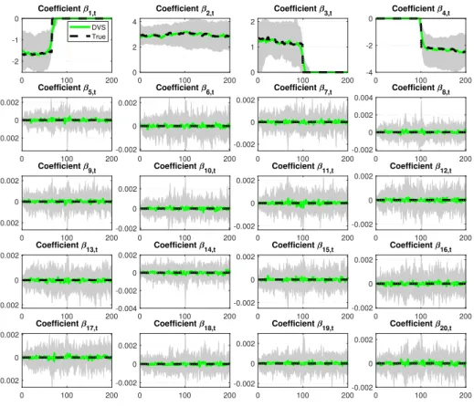
Figure 1: VBDVS coefficient estimates of the first 20 predictors generated from the DGP
with T = 200 and p= 200. Black dashed lines are the true generated coefficients. Posterior
medians (over the 100 Monte Carlo iterations) of VBDVS estimates are shown with green solid lines, and grey areas denote 16th and 84th percentiles.
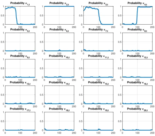
0 100 200 0 0.5 1 Probability 1,t 0 100 200 0 0.5 1 Probability 2,t 0 100 200 0 0.5 1 Probability 3,t 0 100 200 0 0.5 1 Probability 4,t 0 100 200 0 0.5 1 Probability 5,t 0 100 200 0 0.5 1 Probability 6,t 0 100 200 0 0.5 1 Probability 7,t 0 100 200 0 0.5 1 Probability 8,t 0 100 200 0 0.5 1 Probability 9,t 0 100 200 0 0.5 1 Probability 10,t 0 100 200 0 0.5 1 Probability 11,t 0 100 200 0 0.5 1 Probability 12,t 0 100 200 0 0.5 1 Probability 13,t 0 100 200 0 0.5 1 Probability 14,t 0 100 200 0 0.5 1 Probability 15,t 0 100 200 0 0.5 1 Probability 16,t 0 100 200 0 0.5 1 Probability 17,t 0 100 200 0 0.5 1 Probability 18,t 0 100 200 0 0.5 1 Probability 19,t
Time-varying inclusion probabilities
0 100 200
0 0.5 1
Probability 20,t
Figure 2: Time-varying posterior inclusion probabilities (expected value of γj,t estimates) of
the first 20 predictors generated from the DGP withT = 200andp= 200. These probabilities are means over the 100 Monte Carlo iterations.
Figure 1 shows the coefficient estimates from VBDVS for the case T = p = 200. This plot compares the posterior median (green solid lines) versus the true generated coefficients
(black dashed lines). The 16th and 84th percentiles over the 100 Monte Carlo iterations are
also shown as a shaded area around the posterior median. Only the first 20 coefficients, out of the possible 200, are plotted. The first row shows the four coefficients that, at least in some periods, are non-zero, followed by 16 coefficients that are exactly zero. It is impossible to plot the remaining 180 coefficients in the DGP that are exactly zero, but their estimates
are represented fairly well by the estimates of coefficients β5,t - β20,t shown in Figure 1.
Under the assumption of sparsity in the DGP, the VBDVS algorithm is able to recover the true coefficients with accuracy. Not only the coefficients that are zero in the DGP in all periods are correctly estimated to be zero, but also the three coefficients that are zero only in certain subsamples are estimated precisely. When a coefficient is initially zero and later in the sample becomes important (see coefficient β4,t), and vice-versa (see coefficients β1,t
the new state. Figure 2 shows that the true reason why estimation is so precise – even in such a demanding case with 200 time-varying coefficients for only 200 observations – is because the estimates of the time-varying posterior inclusion probabilities (PIPs) of each predictor are recovered with precision in the first instance. By identifying correctly which variables should be excluded from the regression model in each period results in shrinking many coefficients to zero and allowing to preserve enough degrees of freedom for estimation of non-zero coefficients.
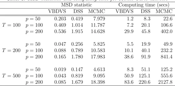
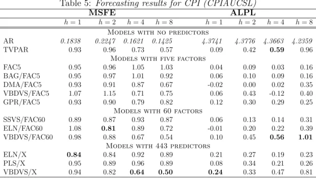
Table 1shows the values of the MSD statistics for the three algorithms under the different
combinations of T and p. Given that the MSD statistics measure deviation from the true
coefficient, lower values imply that a certain estimation algorithm has done better recovery of the coefficients generated by the DGP. In all cases VBDVS has the best performance among all competing algorithms. The estimation error of the MCMC algorithm is quite
large mainly because the algorithm is unable to shrink all p−4 coefficients in the DGP
that are exactly zero. The DSS algorithm provides a better fit since it is also an algorithm that does dynamic variable selection and shrinkage. Its performance is slightly inferior to VBDVS, but the results should not be taken as final evidence. While we have done all effort
to follow the settings suggested byRoˇckov´a and McAlinn(2017), there might be other priors
that could improve the performance of this algorithm.
Another important feature of the VBDVS algorithm is its fast computing time. While it is not surprising that our algorithm is faster compared to MCMC, our algorithm can provide substantial savings in high-dimensional settings compared to the DSS that relies on the EM
algorithm. Columns 6-8 in Table 1 reveals that VBDVS can be multiple times faster than
Table 1: MSD statistics and computing time for Monte Carlo exercise
MSD statistic Computing time (secs)
VBDVS DSS MCMC VBDVS DSS MCMC p= 50 0.203 0.419 7.979 1.2 8.3 22.6 T = 100 p= 100 0.469 1.014 11.787 7.2 20.1 106.6 p= 200 0.536 1.915 14.628 29.9 45.8 402.0 p= 50 0.047 0.256 5.825 5.5 19.9 49.9 T = 200 p= 100 0.088 0.789 10.583 10.1 40.1 232.2 p= 200 0.165 1.780 17.983 38.6 91.9 841.4 p= 50 0.019 0.147 4.613 8.3 51.1 125.2 T = 500 p= 100 0.043 0.819 9.095 50.9 125.1 555.6 p= 200 0.085 1.679 18.398 83.6 220.6 2127.8
Notes: Computing times are based on a Windows 10 laptop running MATLAB 2020a, featuring an Intel i7-8665U processor and 32GB of RAM.
5
Macroeconomic Forecasting with Many Predictors
5.1
A new large dataset for forecasting inflation
Following a large literature on time-varying parameter models in macroeconomics, our primary target is to forecast quarterly US inflation. While there exists mixed empirical evidence about the potential of very large datasets to improve forecasts of inflation, our aim is to demonstrate here that the new dynamic variable selection methodology can successfully extract, period-by-period, predictive information from a large number of predictors. For that reason we build a novel, high-dimensional dataset that brings together predictors from
several mainstream aggregate macroeconomic and financial datasets.12 Our building block
is the FRED-QD dataset of McCracken and Ng (2020), which we augment with portfolio
data used in Jurado et al. (2015), stock market predictors from Welch and Goyal (2007),
survey data from University of Michigan consumer surveys, commodity prices from the World Bank’s Pink Sheet database, and key macroeconomic indicators from the Federal Reserve Economic Data for four economies (Canada, Germany, Japan, UK). All data are quarterly, and span the period 1960Q1-2018Q4. All variables are adjusted from their respective sources
for seasonality (where relevant), and we additionally remove extreme outliers.13
12While one could also think of potential predictors in disaggregated panels obtained in surveys, internet,
or documents (text data), such novel sources are typically proprietary and would make our results hard to replicate.
13Following Stock and Watson (2016), we replace outliers using the median of the preceding five
The dataset has in total 444. Out of these we forecast the series (FRED-QD mnemonics in parentheses): GDP deflator (GDPCTPI), total CPI (CPIAUCSL), core CPI (CPILFESL),
and PCE deflator (PCECTPI). When each of these price series,Pt, is used as the dependent
variable to be forecasted h-quarters ahead we transform it according to the formula yt+h =
(400/h) ln (Pt+h−Pt). We forecast these transformed series one at a time, and the remaining
three price series are included in the list of exogenous predictor variables (443 in total). The predictor variables are transformed using standard norms in the literature (see for example
McCracken and Ng, 2020): i) levels for variables that are already expressed in rates (e.g.
unemployment, interest); ii) first differences of logarithm for variables measuring population (e.g. employment), variables expressed in dollars (e.g. GDP), commodity prices, and some indexes (e.g. Industrial production); and iii) second differences of logarithm for price and consumption indexes, as well as deflator series. The online supplement describes in detail all variables and transformations, and provides links to all sources.
5.2
How the dynamic variable selection algorithm works: An
in-sample assessment
Before we set up a comprehensive out-of-sample forecasting exercise, we first assess in-sample estimates from the VBDVS by doing small sensitivity analysis to various prior choices. This exercise is intended to demonstrate that the new algorithm provides reasonable estimates of trends, volatilities and other parameters. Most importantly it serves as a way to clarify that, despite the fact that our prior is heavily parametrized, prior elicitation in the VBDVS algorithm becomes a reasonably straightforward task. As it is impossible to present estimates of the TVP model using all variables in our dataset as predictors, we focus on a small TVP model where GDP deflator regressed on an intercept, two own lags, and the first five principal components from the 443 exogenous predictors (eight predictors in total).
Out of all parameters and hyperparameters defined in our algorithm it is only a handful that are crucial for inference and forecasting, while others can be fixed to reasonable
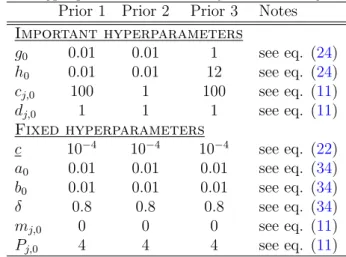
or uninformative values and possibly have little effect on forecasting. Table 2 lists all
hyperparameters one need to choose in the VBDVS algorithm, and does an explicit separation
into “Important” and “Fixed” hyperparameters. Starting from the latter, a0 and b0 are the
initial scale and rate parameters of the initial condition of the precision parameter in equation
(34). Setting a0 =b0 = 0.01 implies that the precision has prior mean one and variance 10,
which is a reasonable uninformative choice for an inverse variance parameter. Next, we set
δ = 0.8 for reasons explained in subsection 3.2. Given that p is very large to allow us to
obtain meaningful prior information about the regression coefficientsβt(e.g. using a training
sample), we allow their initial condition β0 to be fairly uninformative by setting m0 = 0
and P0 = 4Ip. The parameter c in the dynamic variable selection prior has to be small
(see discussion in subsection 3.1) and how small it exactly is, affects the way the algorithm
selects each of the two Normal components in the spike and slab prior – that is, it affects
the choice between a certain βj,t being restricted or not. We prefer to fix this parameter to
c= 0.0001 and allow only τ2
j,t and its prior to determine the ratio of the prior variances of
the two Normal components in the mixture prior.
Table 2: Hyperparameter choices for sensitivity analysis
Prior 1 Prior 2 Prior 3 Notes
Important hyperparameters g0 0.01 0.01 1 see eq. (24) h0 0.01 0.01 12 see eq. (24) cj,0 100 1 100 see eq. (11) dj,0 1 1 1 see eq. (11) Fixed hyperparameters c 10−4 10−4 10−4 see eq. (22) a0 0.01 0.01 0.01 see eq. (34) b0 0.01 0.01 0.01 see eq. (34) δ 0.8 0.8 0.8 see eq. (34) mj,0 0 0 0 see eq. (11) Pj,0 4 4 4 see eq. (11)
The parameters that are important in our high-dimensional setting are the ones affecting
the two prior variances of the time-varying coefficientsβt, namely the hyperparameters ofτ2
j,t
andwj,t. Our first prior choice, denoted as “Prior 1” inTable 2, selectscj,t = 100, dj,t = 1 such
thatwj,thas a prior mean of 0.01 and prior variance 0.0001. This conservative choice restricts
movements βj,t to be very persistent and excludes the case of frequent, noisy jumps. Such
prior is used widely in empirical macroeconomic applications, see for example the “business
as usual” prior motivated inCogley and Sargent(2005) for the case of a vector autoregression
with time-varying parameters. We subsequently set an uninformative prior onτ2
j,t by setting
g0 =h0 = 0.01. The dashed lines inFigure 3represent (posterior mean) coefficient estimates
from our eight-predictor model: coefficientβ1,t is the time-varying intercept (trend inflation),
coefficientsβ2,t, β3,tcorrespond to the first two lagged values of GDP deflator, and coefficients
β4,t to β8,t correspond to the five principal components. As a comparison, we plot posterior
mean estimates from the same time-varying parameter regression estimated with MCMC (using identical settings as in the Monte Carlo comparison). The MCMC-based estimates can be broadly thought of as the unrestricted equivalents of the VBDVS algorithm, since
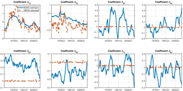
they are not based on any form of dynamic variable selection or hierarchical shrinkage. The intercept and first lag coefficients are virtually identical using the two algorithms. However, all remaining coefficients are penalized heavily by the VBDVS algorithm. Variation over time of these coefficients is very moderate and restricted to be close to zero for many time periods. 1976Q1 1991Q1 2006Q1 -1.5 -1 -0.5 0 0.5 1 Coefficient 1,t MCMC estimate VBDVS estimate 1976Q1 1991Q1 2006Q1 -0.4 -0.2 0 0.2 0.4 0.6 0.8 Coefficient 2,t 1976Q1 1991Q1 2006Q1 -0.4 -0.2 0 0.2 0.4 0.6 0.8 Coefficient 3,t 1976Q1 1991Q1 2006Q1 -0.2 0 0.2 0.4 0.6 Coefficient 4,t 1976Q1 1991Q1 2006Q1 -0.4 -0.2 0 0.2 0.4 Coefficient 5,t 1976Q1 1991Q1 2006Q1 -1 -0.5 0 0.5 Coefficient 6,t 1976Q1 1991Q1 2006Q1 -0.4 -0.2 0 0.2 0.4 0.6 Coefficient 7,t Posterior mean estimate of time-varying coefficients, Prior 1
1976Q1 1991Q1 2006Q1 -0.3 -0.2 -0.1 0 0.1 0.2 Coefficient 8,t
Figure 3: Posterior means of time-varying coefficient estimates from VBDVS (red dashed
lines) using Prior 1. Solid lines are posterior means from a TVP model with the same predictors estimated with MCMC.
In order to examine the effect that the prior has on the time evolution of the coefficients,
we change the initial condition for wj,t to have hyperparameters cj,0 = dj,0 and we leave
the same uninformative prior for τ2
j,t. The posterior mean coefficient estimates in Figure 4
exhibit an interesting pattern. By allowing a looser prior on wt the parameters that are
unrestricted (intercept and first lag), do exhibit larger amount of time-variation compared to the MCMC estimates. However, the remaining coefficients that were previously restricted to be close to zero, are now forced more aggressively towards zero in all time periods. This
demonstrates the fact that our algorithm imposes the state-space model in equation (28),
where the variance of βj,t is a function of both wj,t and vj,t (where the latter, is in turn a
linear function of τ2
j,t). Therefore, allowing for a looserwj,t tends to introduce more noise in
the state-space model, and for that reason the dynamic variable selection prior compensates for this increased noise by shrinking more aggressively. While there is this compensation effect and coefficient estimates won’t explode as quickly as the model without the dynamic
advisable to use such a lose prior on wj,t. 1976Q1 1991Q1 2006Q1 -2 -1 0 1 2 Coefficient 1,t MCMC estimate VBDVS estimate 1976Q1 1991Q1 2006Q1 -1 -0.5 0 0.5 1 Coefficient 2,t 1976Q1 1991Q1 2006Q1 -0.2 -0.1 0 0.1 0.2 0.3 0.4 Coefficient 3,t 1976Q1 1991Q1 2006Q1 -0.2 -0.1 0 0.1 0.2 0.3 0.4 Coefficient 4,t 1976Q1 1991Q1 2006Q1 -0.1 0 0.1 0.2 0.3 0.4 Coefficient 5,t 1976Q1 1991Q1 2006Q1 -0.3 -0.2 -0.1 0 0.1 Coefficient 6,t 1976Q1 1991Q1 2006Q1 -0.4 -0.3 -0.2 -0.1 0 0.1 0.2 Coefficient 7,t
Posterior mean estimate of time-varying coefficients, Prior 2
1976Q1 1991Q1 2006Q1 -0.3 -0.2 -0.1 0 0.1 0.2 Coefficient 8,t
Figure 4: Posterior means of time-varying coefficient estimates from VBDVS (red dashed
lines) using Prior 2. Solid lines are posterior means from a TVP model with the same predictors estimated with MCMC.
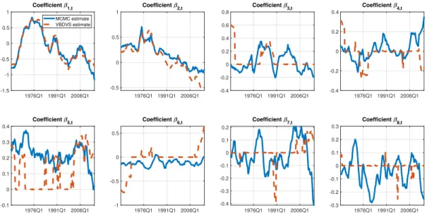
For that reason, our final prior (called Prior 3 in Table 2) returns to the conservative
choice cj,0 = 100 and dj,0 = 1, and sets instead g0 = 1 and h0 = 12. Figure 5 shows
the estimates from this prior. Once again the VBDVS estimates of the intercept and first lag coefficients are identical to the estimates from the MCMC algorithm. The remaining coefficients are again heavily penalized but there are also many time periods where these evolve unrestrictedly. As a matter of fact, this prior allows the time-varying coefficients to exhibit distinct and abrupt jumps between periods where they are zero and periods where they are unrestricted. This pattern of time-variation is more in line with the findings of the previous literature that there are pockets of predictability or, put differently, that economic predictors are short-lived (see discussion in the Introduction).
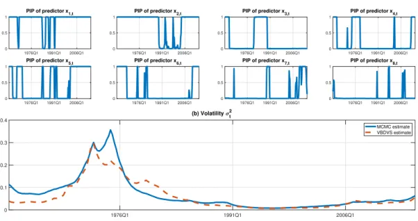
In order to have a visual assessment of the time pattern of dynamic variable selection and
shrinkage, panel (a) of Figure 6 plots the posterior inclusion probabilities of each regressor
associated with the time-varying coefficient estimates presented in Figure 5. These seem to
show the exact periods where each coefficient moves from a state of being restricted to zero to a state where it is not zero. Panel (b) of the same figure shows the posterior mean of the stochastic volatility estimate from VBDVS versus the estimate from MCMC. These two estimates are fairly similar, showing that the specification of time-varying variances in the VBDVS does a good job at capturing known peaks in GDP deflator inflation volatility. Any
differences in volatility estimates reflect the fact that the two algorithms assume different specification of σ2
t and also use different priors in the estimation ofβt.
For all these reason, we build all of our forecasting models in the next subsection based on this last prior.14
1976Q1 1991Q1 2006Q1 -1.5 -1 -0.5 0 0.5 1 Coefficient 1,t MCMC estimate VBDVS estimate 1976Q1 1991Q1 2006Q1 -0.5 0 0.5 1 Coefficient 2,t 1976Q1 1991Q1 2006Q1 -0.4 -0.2 0 0.2 0.4 0.6 0.8 Coefficient 3,t 1976Q1 1991Q1 2006Q1 -0.4 -0.2 0 0.2 0.4 Coefficient 4,t 1976Q1 1991Q1 2006Q1 -0.1 0 0.1 0.2 0.3 0.4 Coefficient 5,t 1976Q1 1991Q1 2006Q1 -1 -0.5 0 0.5 Coefficient 6,t 1976Q1 1991Q1 2006Q1 -0.4 -0.3 -0.2 -0.1 0 0.1 0.2 Coefficient 7,t
Posterior mean estimate of time-varying coefficients, Prior 3
1976Q1 1991Q1 2006Q1 -0.3 -0.2 -0.1 0 0.1 0.2 0.3 Coefficient 8,t
Figure 5: Posterior means of time-varying coefficient estimates from VBDVS (red dashed
lines) using Prior 3. Solid lines are posterior means from a TVP model with the same predictors estimated with MCMC.
14Due to the fact that the choice h
0 = 12 looks in Figure 5 to penalize possibly excessively the small
model with just eight coefficients, in the next subsection we adapt only this hyperparameter depending on the number of predictors we have available. Otherwise, all other hyperparameters are identical to the ones in the column labelled Prior 3 inTable 2.
1976Q1 1991Q1 2006Q1 0 0.5 1 PIP of predictor x1,t 1976Q1 1991Q1 2006Q1 0 0.5 1 PIP of predictor x2,t 1976Q1 1991Q1 2006Q1 0 0.5 1 PIP of predictor x3,t 1976Q1 1991Q1 2006Q1 0 0.5 1 PIP of predictor x4,t 1976Q1 1991Q1 2006Q1 0 0.5 1 PIP of predictor x5,t 1976Q1 1991Q1 2006Q1 0 0.5 1 PIP of predictor x6,t 1976Q1 1991Q1 2006Q1 0 0.5 1 PIP of predictor x7,t
(a) Posterior inclusion probabilities
1976Q1 1991Q1 2006Q1 0 0.5 1 PIP of predictor x8,t 1976Q1 1991Q1 2006Q1 0 0.1 0.2 0.3 0.4 (b) Volatility t2 MCMC estimate VBDVS estimate
Figure 6: Panel (a) shows time-varying posterior inclusion probabilities (PIPs) from VBDVS
algorithm, using Prior 3. Panel (b) shows posterior means of time-varying volatility estimates from VBDVS (red dashed line) versus MCMC (solid blue line).
5.3
Forecasting inflation
We forecast inflation using models of the form
yt+h =αt+φ1,tyt+φ2,tyt−1+xtβt+εt+h, (45)
where yt+h is h-step ahead inflation (see subsection 5.1 for a definition) regressed on an
intercept, two own lags and exogenous predictors. We use a variety of forecasting models.
Some benchmark models are based on equation (45) but assume constant coefficients (i.e.
αt = α, φ1,t = φ1 and so on), while others assume different sets of exogenous predictors.
However, what all models have in common is that they always include an intercept and two own lags of inflation. Given that our dataset is much larger than datasets used before for forecasting inflation, in order to avoid confusion by specifying different combinations or subsets of predictors, we only distinguish four simple categories of models: i) models with no predictors (i.e. only intercept and autoregressive terms); ii) models with first five principal components as predictors; iii) models with sixty principal components as predictors; and iv) models with all 443 predictors. Our list of models representing each category is the following
❼ AR: benchmark AR(2) with intercept, estimated with OLS
estimated with MCMC
❼ FAC5: Builds on benchmark AR specification by augmenting it with first five principal components estimated with OLS
❼ BAG/FAC5: Same predictors as FAC5, estimated as constant parameter regression
using the Bagging algorithm of Breiman (1996)
❼ DMA/FAC5: Same predictors as FAC5, estimated as TVP regression using the
Dynamic Model Averaging algorithm ofKoop and Korobilis (2012)
❼ VBDVS/FAC5: Same predictors as FAC5, estimated as TVP regression using our Dynamic Variable Selection prior with Variational Bayes
❼ GPR/FAC5: Same predictors as FAC5, estimated as a Gaussian Process Regression ❼ SSVS/FAC60: Builds on benchmark AR specification by augmenting it with first
60 principal components, estimated using the SSVS prior with MCMC of George and
McCulloch (1993)
❼ ELN/FAC60: Same predictors as SSVS/FAC60, estimated as a constant parameter
regression using the Elastic Net algorithm of Zou and Hastie(2005)
❼ VBDVS/FAC60: Same predictors as SSVS/FAC60, estimated as a TVP regression using our Dynamic Variable Selection prior with Variational Bayes
❼ ELN/X: Builds on benchmark AR specification by augmenting it with all 443
predictors, estimated using the Elastic Net algorithm of Zou and Hastie(2005)
❼ PLS/X: Same predictors as in ELN/X, estimated as a constant parameter Partial Least Squares regression
❼ VBDVS/X: Same predictors as ELN/X, estimated as a TVP regression using our Dynamic Variable Selection prior with Variational Bayes
The choice of models is based on their simplicity and replicability. In particular, the Gaussian Process Regression, Partial Least Squares, and Elastic Net algorithms are based on built-in
functions in MATLAB’s Statistics and Machine Learning Toolbox (MATLAB,2020), and are
fairly easy to set up. Estimation of these models is done using default settings in MATLAB
or default choices proposed by their respective creators.15 Exact details of these algorithms
and their default settings is provided in the Online Supplement.
In terms of statistical properties, all these models cover a wide spectrum of forecasting specifications. The AR(2) is a standard benchmark in economic time series forecasting, and typically performs better than a random walk (which is the benchmark for financial data). Its time-varying parameter counterpart, our second model on the list, allows for proxying for
similar specifications that have been shown to forecast inflation well, see Stock and Watson
(2007) and Bauwens et al. (2015). Extracting the first few principal components (factors)
is possibly the most popular way of representing parsimoniously the information in a large
dataset, see Stock and Watson (2016). A naive factor model uses least squares estimation
on a model that has the first five principal components as exogenous predictors, while a
second factor model replaces OLS with the Bagging algorithm ofBreiman(1996) that allows
to select the “best” factors in a static way. Next the Dynamic Model Averaging (DMA)
algorithm described in Koop and Korobilis(2012) as well as our VBDVS algorithm allow to
implement dynamic variable selection in a TVP setting using the same first five principal components. The Gaussian Process Regression is a very flexible nonparametric method that allows us to understand whether inflation is better described by time-varying parameters or some more complex form of nonlinearity. Moving on to models with 60 factors, we have
to drop many previous specifications for computational reasons.16 For that reason we use
the SSVS algorithm ofGeorge and McCulloch (1993), which can be thought of as the static
equivalent of our VBDVS algorithm. The Elastic Net ofZou and Hastie (2005) is a popular
penalized likelihood estimator for high-dimensional data. Finally, our VBDVS algorithm is also estimated with a larger number of factors to find out whether its dynamic shrinkage properties are useful relative to the naive selection of the first five factors. Finally, we estimate models using all 443 exogenous predictors. The Elastic Net is again on the list, and we also include Partial Least Squares (PLS) regression. PLS is similar to principal component analysis, with the main difference being that factors are extracted with reference to the variable to be predicted. Principal components instead only explain the variability in the exogenous predictors, and it may be the case that they do not carry predictive information for the predicted variable. Finally, our VBDVS algorithm is applied to this full model with all predictors.
In terms of the prior choices used when forecasting with our VBDVS algorithm, these
are based on Prior 3 described in the previous subsection, see Table 2. We only adapt how
“aggressively” we shrink based on the total number of predictors in each model. For model
VBDVS/FAC5 we set h0 = 1, for VBDVS/FAC60 we set h0 = 12 and for VBDVS/X we set
h0 = 100.
16For example, DMA cannot scale up to these large dimensions, Gaussian Process Regression becomes