On the Identification of Model Error through Observations of
Time-varying Parameters
P.L.Green1, E.Chodora2, S.Atamturktur2
1 Institute for Risk and Uncertainty, School of Engineering,
University of Liverpool, Liverpool, United Kingdom, L69 7ZF
2 Department of Mechanical Engineering, Clemson University,
Clemson, United States, SC 29634
Abstract
When performing system identification, it can be possible to realise a deficient model (i.e. one that will make low fidelity predictions) that is able to closely represent a set of training data. For example, the parameters of linear dynamical models can often be tuned to realise a close match to training data that was generated from a system with strong nonlinearities. Despite this close match to available data, these same models may make very poor-quality predictions when shifted even slightly from the ‘validation domain’ (which could, for example, be a specific time window). In this paper we investigate the hypothesis that, by treating our model’s parameters as being time-varying, we can identify key weaknesses in a model that would have been difficult to establish using other identification methods that do not consider the potentially time-varying nature of the model’s parameters. Specifically, we use an Extended Kalman Filter to ‘track’ the parameters of a dynamical system, as a time history of training data is analysed. We then illustrate that this approach can reveal important information about the potential deficiencies of a model.
1
Introduction
Computational models are crucial to many fields of science and engineering. Before being used to influence decision-making, such models must be validated; it must be established that the model can represent the real world with a level of accuracy sufficient for its intended purpose. Model validation is, as a result, an active research area.
In a broad sense, the current paper considers the situation where:
1. our chosen model structure features a set of parameters that will need to be ‘tuned’ during the validation process.
2. a set of observations, from the system of interest, are available to the user (such that this data can be used to help infer parameter estimates).
While such scenarios are considered by much of the literature, the current paper differs from most in that it explicitly considers the issues associated withextrapolation. Specifically, by ‘extrapolation’ we are referring to a situation where a model will be used to make predictions in a region that is ‘very far’ from current experimental observations - a region where there is no observation data (and it may be difficult to collect data in the future). Using the terminology given in [1], we are essentially considering the situation where a model must be applied outside of its ‘domain of applicability’. Inevitably then, we must ask the question: will the model make valid extrapolations?
Answering such a question is extremely difficult. Furthermore the problem is often confounded by the fact that, in the regions where measurements are available, calibration can mask model error. In other words, a model’s parameters can often be tuned such that the model appears to be sufficiently valid compared to the available data, even if the model will be a poor extrapolator (we show an illustrative example of this in section 4.2 of the current paper). The current work presents an approach that can, in such a scenario, illustrate the flaws in a model; warning us that the model should not be used for extrapolative predictions.
Briefly, our approach is as follows. Firstly, we limit ourselves to situations where we believe our model of interest’s parameters should be time-invariant. We then adopt a calibration procedure that deliber-ately treats these parameters as being time-varying, even though we believe this is not the case. It is by observing that a model’s parameters must vary with time if it is to replicate a set of measurements with a high level of fidelity that we aim to identify key discrepancies in the model that may be hidden by other calibration procedures. We believe that, for future work, the approach can form part of validation frameworks such as those described in [2] [3].
2
Literature Review
The idea that statistical models can be used to emulatemodel discrepancy(see [4] and [5] for example) has influenced a large body of work. This approach accepts that there will always be a discrepancy between a model that is formulated on our best understanding of the system of interest (a model that is based on physical laws, for example) and the system’s true response. A purely data-based model is then trained and used to realise predictions of this discrepancy. Subsequent to calibration, then, predictions are made using a combination of the model that is based on our best understanding of the system and the data-based discrepancy model1.
One of the best-known implementations of this approach is that of Kennedy and O’Hagan [4], where Gaussian Processes (GPs) were used to create statistical models of model discrepancy (as well as em-ulators, for the cases where simulations of the system of interest are expensive). This idea has con-tributed to many works in the field of model validation. These include generalised validation frame-works [6] [7] [8], model validation metrics that consider model discrepancy [1], metrics to establish when sufficient experimental data has been gathered in the model validation process [9] and approaches for resource allocation (between code development and experimental testing [10] or the development of substructures within a model [11]).
While undoubtedly a useful contribution, employing data-based models of discrepancy cannot help im-prove extrapolations that are far from the training data (GPs, for example, will return very quickly to predictions based only on prior knowledge of the discrepancy if used in a region where there is no data). This issue is highlighted by a number of authors. In [12] it is stated that ‘the primary use of engineering models is to extrapolate to a system with new nominals when there are no new field data’
1
This type of approach is sometimes called grey-box modelling, as it utilises a combination of a ‘white box model’ (model based on our understanding of the system) and a ‘black box model’ (a model that is purely data-based).
but that extrapolation, using the approach described in [4], can only be performed if there is a ‘modest’ change in the inputs. The authors of [2] note that ‘such a statistically adjusted engineering model lacks predictive power in the sense that it can be used only in the experimental conditions identical or very similar to those under which the statistical model was fitted’ and in [3] it is stated that ‘...the discrepancy representation ... is highly dependent on calibration against observables and, hence, should not be used in situations in which it cannot be trained and tested’.
At this point it is important to note that the above discussion isn’t a direct critisism of [4] - the authors did not claim that the method will provide reliable extrapolations. In fact, an interesting discussion of the Kennedy and O’Hagan approach is given by Brynjarsdóttir and O’Hagan in [13], which considers how the use of GP emulators of model discrepancy can (1) aid the identification of a system’s ‘true’ parameter values and (2) aid extrapolations. It is concluded that true parameter values can only be un-covered if realistic prior information about the model discrepancy is available and that, even if realistic prior information is available, extrapolation is not advisable. [13] highlights these two issues nicely us-ing a simple case study.
To further clarify the position of our paper in current literature, it is stressed that we are considering the situation where, in the region we wish to make predictions, there is no data (and we don’t expect there to be any data in the future). This consideration separates the current paper from [1] and [9] that (respectively) describe a ‘predictive maturity index’ and a ‘forecasting metric’, as these approaches utilise hold-out experiments (experimental observations, in the application domain, that are deliberately removed from the training data so that they can be used to aid validation at a later stage). Instead, we propose a method that can, potentially, be used to reveal additionalengineering knowledgeabout a par-ticular system. For future work, we aim to utilise this method as part of the frameworks described in [2] and [3], both of which specifically consider extrapolation.
3
Methodology
3.1 General Framework
As stated previously, the current work specifically concerns the analysis of dynamical systems. Using
xi to represent a system’s state at timei∆tthen, generally, we propose that the system’s state evolves according to
xi=f(xi−1,ui) +vi−1, vi−1 ∼ N(vi−1;0,Qi−1) (1)
where∆tis a fixed time increment, ui is a system input, f is a model that predicts the next system state given(xi−1,ui)andvi−1is a ‘noise term’ that reflects the uncertainties in our predictions of the
system’s next state (arising becausef is an approximation of the true system). Equation (1) is typically referred to as the ‘prediction equation’.
Likewise, usingzito represent an observation of some aspect of our system at timei∆t, we also suppose that measurements are made according to
zi =hi(xi) +ni, ni ∼ N(ni;0,Ri) (2)
wherehis a (potentially nonlinear) function of the system’s state andni is used to capture uncertainty in the observation process (measurement noise). Equation (2) is typically referred to as the ‘observation equation’. We note that, in the literature, the prediction and observation equations are often written as potentially nonlinear functions of their noise terms (vi−1andnirespectively) - we have neglected to do so here for notational simplicity later in the paper.
3.2 Extended Kalman Filter
Now consider the situation where the aim is to probabilistically ‘track’ how the state of our system changes with time, as more observations arrive over time. If, in our prediction and observation equa-tions,f andhare linear functions ofxi−1 andxirespectively then it is possible to realise closed-form solutions for this problem. These solutions form the well-known Kalman filter.
Iff andhare nonlinear then, generally, such closed-form solutions are unavailable. One way to address this is to approximatef andhusing linear functions (via first-order Taylor series expansions), before applying the ‘standard’ Kalman filter equations to the new, linearised relationships. This approach is called the Extended Kalman Filter (EKF)2.
Here we give a brief description of an extended Kalman filter, to establish notation used later in the paper. Firstly we define:
Fxˆ ≡ [ ∂f ∂x ] x=ˆx (3) and Hxˆ ≡ [ ∂h ∂x ] x=ˆx (4) Now, say it is currently assumed that
p(xi−1|z1:i−1) =N(xi−1;mi−1|i−1,Pi−1|i−1) (5)
such that the probability density function (PDF) ofxi−1 givenz1:i−1is Gaussian with meanmi−1|i−1
and covariance matrixPi−1|i−1. With an EKF we first use our linearised prediction equation to predict
the next system state. This yields the PDF
p(xi|z1:i−1) =N(xi;mi|i−1,Pi|i−1) (6)
Once a new observation arrives (zi) then, through our observation equation, we can update our estimate of the system state to obtain:
p(xi|z1:i) =N(xi;mi|i,Pi|i) (7) where the parameters of the PDFs in equations (5), (6) and (7) are as follows:
mi|i−1 =f(mi−1|i−1) (8) Pi|i−1 =Qi−1+Fmi−1|i−1Pi−1|i−1F T mi−1|i−1 (9) mi|i=mi|i−1+Ki(zi−h(mi|i−1)) (10) Pi|i =Pi|i−1−KiHmi|i−1Pi|i−1 (11) 2
There are many other ways in which this problem could be tackled. One of the most well-known is theparticle filter- a numerical method that is fundamentally based on importance sampling (see [14] for a tutorial). Here, however, we found that an extended Kalman filter performed acceptably well and that our prediction and measurement equations were not sufficiently nonlinear to warrant use of a particle filter.
and Ki =Pi|i−1HTmi|i−1S −1 i (12) Si=Hmi|i−1Pi|i−1H T mi|i−1 +Ri (13)
3.3 Application to the 4th order Runge-Kutta integration scheme
In the following we consider a dynamical system that may be subjected to a time history of known excitations: δ1,δ2, .... The state of these systems is calculated recursively using the 4th order
Runge-Kutta numerical integration scheme. To help us relate this scheme back to the general ‘prediction equation’ shown in equation (1), we must make some additional notation. Firstly, we write
ui = ( δi−1 δi ) (14) Secondly, we establish the notation
˙ x(xi,δi)≡ [ ∂x ∂t ] x=xi,δ=δi (15) and define k1 = ˙x(xi−1,δi−1) (16) k2= ˙x ( xi−1+ ∆t 2 k1,δint ) (17) k3= ˙x ( xi−1+ ∆t 2 k2,δint ) (18) k4 = ˙x(xi−1+∆tk3,δi) (19)
where∆tis the time-step of our integration scheme andδint= 12(δi−1+δi). Using this notation, the functionf that mapsxi−1toxican be written as
xi =xi−1+
∆t
6 (k1+2k2+2k3+k4) (20)
We now need to find an expression forFxˆ (equation (3)). We note that
Fxˆ =I+ ∆t 6 [ ∂k1 ∂xi−1 ] xi−1=ˆx | {z } Term 1 +2 [ ∂k2 ∂xi−1 ] xi−1=ˆx | {z } Term 2 +2 [ ∂k3 ∂xi−1 ] xi−1=ˆx | {z } Term 3 + [ ∂k4 ∂xi−1 ] xi−1=ˆx | {z } Term 4 (21) Evaluation of terms 1-4 in equation (21) essentially requires the application of some straightforward vector calculus. For the sake of completeness, the required derivatives are shown in detail in Appendix A. Ultimately, we find that
[ ∂k1 ∂xi−1 ] xi−1=ˆx = ˜F(ˆx,δi−1) (22)
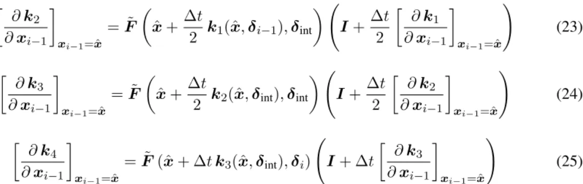
[ ∂k2 ∂xi−1 ] xi−1=ˆx = ˜F ( ˆ x+∆t 2 k1(ˆx,δi−1),δint ) ( I +∆t 2 [ ∂k1 ∂xi−1 ] xi−1=ˆx ) (23) [ ∂k3 ∂xi−1 ] xi−1=ˆx = ˜F ( ˆ x+∆t 2 k2(ˆx,δint),δint ) ( I +∆t 2 [ ∂k2 ∂xi−1 ] xi−1=ˆx ) (24) [ ∂k4 ∂xi−1 ] xi−1=ˆx = ˜F (ˆx+ ∆tk3(ˆx,δint),δi) ( I+ ∆t [ ∂k3 ∂xi−1 ] xi−1=ˆx ) (25) where we have usedF˜(x,δ)to represent the Jacobian ofx˙, with respect toxi−1, evaluated at the points xandδ.
4
Numerical Case Study
4.1 Description
We consider modelling a single degree of freedom nonlinear dynamic system whose equation of motion is
¨
x+cx˙+kx+k∗x3 =δ(t) (26) In equation (26)x is displacement, cis a linear damping coefficient,kis a linear stiffness coefficient andk∗is a nonlinear stiffness coefficient that controls the strength of the system’s ‘hardening’ stiffness nonlinearity. δ(t)is a random excitation that, in this case, consists of samples drawn from a zero-mean unit-variance Gaussian.
To generate a set of ‘observation data’ the nonlinear system was simulated using a time step of∆t = 0.01s. Observations were created by taking the resulting displacement time history and corrupting it with Gaussian noise (variance1×10−5). The model’s parameters were k = 10 N/m,c = 0.1 Ns/m andk∗ = 50N/m3. Observation data was generated over a time period of 200 seconds. The full set of
observation data is shown in Figure 1 while a zoomed-in portion is shown in Figure 2.
0 20 40 60 80 100 120 140 160 180 200 Time (s) -0.2 -0.15 -0.1 -0.05 0 0.05 0.1 0.15 0.2 Displacement (m) Observed True
Figure 1: 200 seconds of displacement time history observations from the numerical case study. Black shows the true response of the system while red shows noisy observations.
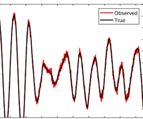
10 12 14 16 18 20 22 24 26 Time (s) -0.06 -0.04 -0.02 0 0.02 0.04 0.06 0.08 0.1 0.12 Displacement (m) Observed True
Figure 2: Numerical case study. A close-up view of the data shown in Figure 1.
In the following we will first consider the case where we are incorrectly attempting to fit a linear model to data that is obtained from the nonlinear system. We will also consider that, after calibration, the model will be used to predict the response of the system to a much greater amplitude excitation than that used to generate the data in Figure 1.
We have deliberately considered a situation where the excitation used to generate the observation data is relatively low, such that the nonlinearity is difficult to detect. Before exploring our methodology for detecting model deficiencies we will illustrate that, by tuning its parameters, this is a situation where we can make our linear model represent the data from the nonlinear system fairly accurately (Section 4.2), potentially giving false confidence in the model’s ability to extrapolate. Our potential solution is then demonstrated in Section 4.3.
4.2 Highlighting the Problem
Here we adapt a common Bayesian approach to the calibration of the model, where it is assumed that the model’s parameters are time-invariant. The results highlight some of the issues that can arise when the model is required for extrapolation. The approach begins with Bayes’ theorem:
p(θ|D)∝p(D|θ)p(θ) (27) whereθis the vector of parameters to be calibrated andDrepresents training data (in this caseDis a time history of the excitation and the observed displacement response of our system). The likelihood, p(D|θ), is defined based on the assumption that each of our observations are equal to the response of the model, corrupted by the addition of Gaussian noise. This noise is assumed to be zero-mean, have varianceRand be independent of the noise that corrupted previous observations. Furthermore, we treat Ras a time-invariant parameter that also requires calibration. Consequently, we haveθ= (k, c, R)T.
By defining the likelihood in this way we are treating any differences between what we observe and what the model predicts (i.e. errors that arise because of both measurement noise and model discrep-ancy) as independent Gaussian noise3. Moreover, by allowingR to be calibrated, we are also tuning the variance of this noise while simultaneously tuning the model’s stiffness and damping parameters. This framework means that the maximum likelihood set of model parameters are those that make the discrepancy between the model and the observations most closely approximate a Gaussian distribution with varianceR. This way of treating uncertainty in the calibration procedure has been applied by many (including the author’s of the current manuscript) and is referred to in [13] as a ‘traditional approach’.
3
This assumption is often justified by the principle of maximum entropy [15], although [16] highlights examples where prediction errors can be spatially and/or temporally correlated.
In the academic example discussed herein, prior distributions over the calibration parameters were cho-sen to be
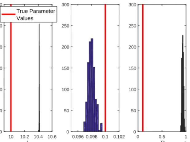
p(k) =N(k; 10,32), p(c) =N(c; 0.1,0.12), p(R) =Gamma(R; 1,100) (28) (such that the prior overR is a Gamma distribution whose shape and rate parameters are equal to 1 and 100 respectively). Using the first 50 seconds of data for training, the Markov chain Monte Carlo (MCMC) algorithm detailed in [17] was used to generate 1000 samples from the posterior,p(θ|D). Histograms of the resulting samples are shown ‘close up’ in Figure 3 while, in Figure 4, histograms are plotted alongside the true parameter values. These results highlight two things. Firstly the posterior distribution overkis concentrated over values that are larger than the true stiffness. This illustrates how khas been calibrated to overcome the model discrepancy (the lack of the nonlinear term). Secondly, the distribution overRis also concentrated on values that are larger than the true measurement noise vari-ance. From these results we can see that this particular approach has attempted to describe the model discrepancy present in the problem as additional noise on our observations (in other words, the errors present in the model has increased the most probable value ofR).
10.4 10.41 10.42 0 50 100 150 200 250 300 Frequency of Samples 0.096 0.098 0.1 0 50 100 150 200 250 8 9 10 10-5 0 50 100 150 200 250
Figure 3: Histograms of samples from the posterior parameter distribution of the linear model in the numerical case study. All parameters in SI units.
10 10.2 10.4 10.6 0 50 100 150 200 250 300 Frequency of Samples True Parameter Values 0.096 0.098 0.1 0.102 0 50 100 150 200 250 300 0 0.5 1 10-4 0 50 100 150 200 250 300
Figure 4: Histograms of samples from the posterior parameter distribution of the linear model in the numerical case study. True parameter values are marked by red lines. All parameters in SI units.
An illustration of the problem that motivates the current paper comes when the MCMC samples are used to propagate our parameter uncertainties into future model predictions. Recalling that we only have data in a relatively low amplitude regime, Figure 5 shows the model’s predictions relative to (1) the training data and (2) data that was ‘held back’ for validation purposes. Figure 6 shows a close-up of the model’s
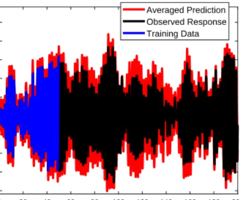
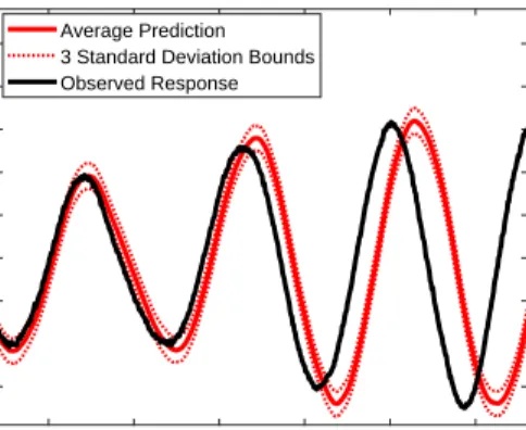
ability to replicate previously unseen data. These results illustrate that, for low amplitude excitations, the model is able to closely replicate data that was not used in training. This then, highlights the prob-lem: the model has been tuned to work effectively in the region where we have data, however, because we have not included the hardening-stiffness nonlinearity, it will perform badly if used to predict the system’s response at high amplitudes. To demonstrate this degradation in performance, the model was used to predict the response of the system to a higher amplitude excitation, wherebyδ(t)consisted of samples drawn from a zero-mean Gaussian whose standard deviation was equal to 2. Figure 7 illustrates that, for this higher amplitude excitation, the model is not able to accurately replicate the response of the system (or accurately quantify the uncertainties involved in the predictions). Our main argument here is that, without the high amplitude response data, it is difficult to diagnose the errors in the model and infer that this model would be a poor extrapolator.
0 20 40 60 80 100 120 140 160 180 200 Time (s) -0.2 -0.15 -0.1 -0.05 0 0.05 0.1 0.15 0.2 0.25 Displacement (m) Averaged Prediction Observed Response Training Data
Figure 5: Propagating parameter uncertainties of the linear model into predictions (numerical case study). Blue represents training data, black represents previously unseen data and red represents the average model predictions. Bounds on model predictions are 3 standard deviations from the mean.
69 70 71 72 73 74 75 Time (s) -0.15 -0.1 -0.05 0 0.05 0.1 0.15 0.2 0.25 Displacement (m) Average Prediction 3 Standard Deviation Bounds Observed Response
Figure 6: Propagating parameter uncertainties of the linear model into predictions of previously unseen, ‘low amplitude’ data. Bounds on model predictions are 3 standard deviations from the mean.
15 16 17 18 19 20 Time (s) -0.3 -0.2 -0.1 0 0.1 0.2 0.3 0.4 0.5 Displacement (m) Average Prediction 3 Standard Deviation Bounds Observed Response
Figure 7: Propagating parameter uncertainties of the linear model into predictions of previously unseen, ‘high amplitude’ data. Bounds on model predictions are 3 standard deviations from the mean.
Below, we outline our proposed approach to the same situation, using the same observation data.
4.3 Proposed Approach
We now consider two separate model structures: M1 and M2. M1 represents the linear model i.e.
the model discussed in the previous section. M2includes the nonlinear stiffness term - it has the same
structure as equation (26) and so, by consideringM2, we are deliberately addressing a situation where
there is no model error. The calibration parameters of M1 and M2 are now written as θ1 and θ2
respectively, such that
θ1= (k, c, R)T, θ2 = (k, c, k∗, R)T (29)
To treat our model’s parameters as being time-varying, we include them in the definition of the system’s state. This allows them to be ‘tracked’, alongside the system’s displacement and velocity, using the EKF (see [18] for a similar approach that utilised particle filtering techniques). Here we illustrate how the approach can be implemented forM2(the model that includes the nonlinear stiffness term), where
the state at timei∆twould bexi = (xi,x˙i, ki, ci, k∗i)T. Implementation of this approach toM1is very
similar and, as such, is not discussed in detail here.
In order to implement the EKF, we must define a model that predicts how our parameters may vary through time i.e. we need to define f in equation (1). As with [18], we assume that each system parameter is equal to its preceeding value, such that
˙ x= ˙ x δ−kx−cx˙−k∗x3 0 0 0 (30)
Consequently, the JacobianF˜ is given by
˜ F(x, δ) = 0 1 0 0 0 −(k+ 3k∗x2) −c −x −x˙ −x3 0 0 0 0 0 0 0 0 0 0 0 0 0 0 0 (31)
We must also quantify the uncertainty in this predictive model (in other words we must define the covariance matrixQi−1in equation (1)). Here, we select
Qi−1 = [ 02×2 02×3 03×2 Gi−1 ] (32) whereGi−1is a diagonal matrix that, for modelM2, is of size3×3. Our approach assumes that there is
zero uncertainty associated in the prediction of displacement and velocity, and that all of the uncertainty manifests itself in the prediction of how our parameter estimates vary through time. This is deliberate - it is the tracking of these parameter estimates that, we hope, will give us subtle indications of model error. Following on from [18], we choose the diagonal elements ofGsuch that the coefficient of vari-ation in the drift of each parameter is fixed. For the numerical case study shown here the coefficient of variation was set equal to 0.1 %.
0 20 40 60 80 100 120 140 160 180 8 10 12 Predicted True 0 20 40 60 80 100 120 140 160 180 0.05 0.1 0.15
Figure 8: Tracking time varying parameters for the linear model. Black lines show true parameter values, red lines show estimated parameter values. Bounds on parameter estimates are 3 standard deviations from the mean.
Figure 8 shows the results that were obtained when the parameters of the linear model were treated as time varying, and tracked using the EKF. As we would expect, this method allows the displacement and velocity to be tracked very accurately - a comparison between the observed and predicted is not shown here because the two are essentially indistinguishable. Figure 8 shows that, relatively speaking, the system’s damping value converges while the linear stiffness varies with time.
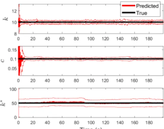
Figure 9: Tracking time varying parameters for the nonlinear model. Black lines show true parameter values, red lines show estimated parameter values. Bounds on parameter estimates are 3 standard deviations from the mean.
0 20 40 60 80 100 120 140 160 180 Time (s) 6 7 8 9 10 11 12 13 14
Without Model Error With Model Error
Figure 10: Tracking the stiffness for the nonlinear model (red) and linear model (blue). Bounds on parameter estimates are 3 standard deviations from the mean.
To aid comparison this analysis was repeated for the nonlinear model. These results are shown in Figure 9 while Figure 10 shows the comparison between the stiffness values that were identified, as a function of time, for both the linear and nonlinear models. To achieve an excellent fit to the observation data we can see that the stiffness of the linear model had to vary significantly more than the stiffness of the nonlinear model. Recall that we are deliberately studying systems whose parameters, we believe, should not be varying with time.
5
Discussion and future work
The question is: do the results in Figure 10 tell us that the linear model would extrapolate poorly if used at high amplitudes? The answer is not straightforward and it is clear that these results would require a significant amount of interpretation. However, we argue that allowing the parameters to vary with time provides a different type of information relative to the more traditional approach shown in Section 4.2. We believe it is conceivable that, by studying the results in Section 4.3, a practitioner may lead to a different set of conclusions about the suitability of the linear model for extrapolations compared to if they had studied the results in Section 4.2 (i.e. the more traditional approach). For future work it seems sensible to combine the proposed approach with a sensitivity analysis. This would help to establish, in a more rigorous manner, whether the witnessed variations in parameter values are truly significant. In particular, combining our approach with a sensitivity analysis of the model in the region where it is to be extrapolated could be an important part of an overall validation framework.
A
Evaluating terms 1-4 in equation (21)
[ ∂k1 ∂xi−1 ] xi−1=ˆx = [ ∂x˙(xi−1,δi−1) ∂xi−1 ] xi−1=ˆx ≡F˜(ˆx,δi−1) (33) Defining s2 =xi−1+ ∆t 2 k1(xi−1,δi−1) (34) then [ ∂k2 ∂xi−1 ] xi−1=ˆx = [ ∂x˙(s2,δint) ∂s2 ∂s2 ∂xi−1 ] xi−1=ˆx (35)
= [ ∂x˙(s2,δint) ∂s2 ] s2=ˆx+∆2tk1(ˆx,δi−1) ( I+∆t 2 [ ∂k1 ∂xi−1 ] xi−1=ˆx ) (36) = ˜F ( ˆ x+∆t 2 k1(ˆx,δi−1),δint ) ( I +∆t 2 [ ∂k1 ∂xi−1 ] xi−1=ˆx ) (37) Likewise, defining s3 =xi−1+ ∆t 2 k2(xi−1,δint) (38) allows us to write [ ∂k3 ∂xi−1 ] xi−1=ˆx = [ ∂x˙(s3,δint) ∂s3 ∂s3 ∂xi−1 ] xi−1=ˆx (39) = [ ∂x˙(s3,δint) ∂s3 ] s3=ˆx+∆2tk2(ˆx,δint) ( I +∆t 2 [ ∂k2 ∂xi−1 ] xi−1=ˆx ) (40) = ˜F ( ˆ x+∆t 2 k2(ˆx,δint),δint ) ( I +∆t 2 [ ∂k2 ∂xi−1 ] xi−1=ˆx ) (41) Finally, writing s4 =xi−1+∆tk3(xi−1,δint) (42) we have [ ∂k4 ∂xi−1 ] xi−1=ˆx = [ ∂x˙(s4,δi) ∂s4 ∂s4 ∂xi−1 ] xi−1=ˆx (43) = [ ∂x˙(s4,δi) ∂s4 ] s4=ˆx+∆tk3(ˆx,δint) ( I+ ∆t [ ∂k3 ∂xi−1 ] xi−1=ˆx ) (44) = ˜F (ˆx+ ∆tk3(ˆx,δint),δi) ( I+ ∆t [ ∂k3 ∂xi−1 ] xi−1=ˆx ) (45)
References
[1] F. Hemez, H.S. Atamturktur, and C. Unal. Defining predictive maturity for validated numerical simulations.Computers & structures, 88(7-8):497–505, 2010.
[2] V.R. Joseph and H. Yan. Engineering-driven statistical adjustment and calibration.Technometrics, 57(2):257–267, 2015.
[3] T.A. Oliver, G. Terejanu, C.S. Simmons, and R.D. Moser. Validating predictions of unobserved quantities.Computer Methods in Applied Mechanics and Engineering, 283:1310–1335, 2015. [4] M.C. Kennedy and A. O’Hagan. Bayesian calibration of computer models. Journal of the Royal
Statistical Society: Series B (Statistical Methodology), 63(3):425–464, 2001.
[5] M. Goldstein and J. Rougier. Probabilistic formulations for transferring inferences from mathe-matical models to physical systems.SIAM journal on scientific computing, 26(2):467–487, 2004.
[6] M.J. Bayarri, J.O. Berger, R. Paulo, J. Sacks, J.A. Cafeo, J. Cavendish, C.H. Lin, and J. Tu. A framework for validation of computer models.Technometrics, 49(2):138–154, 2007.
[7] M.J. Bayarri, J.O. Berger, M.C. Kennedy, A. Kottas, R. Paulo, J. Sacks, J.A. Cafeo, C.H. Lin, and J. Tu. Predicting vehicle crashworthiness: Validation of computer models for functional and hierarchical data.Journal of the American Statistical Association, 104(487):929–943, 2009. [8] C. Unal, B. Williams, F. Hemez, S.H. Atamturktur, and P. McClure. Improved best estimate
plus uncertainty methodology, including advanced validation concepts, to license evolving nuclear reactors.Nuclear Engineering and Design, 241(5):1813–1833, 2011.
[9] S. Atamturktur, F. Hemez, B. Williams, C. Tome, and C. Unal. A forecasting metric for predictive modeling.Computers & Structures, 89(23-24):2377–2387, 2011.
[10] S. Atamturktur, J. Hegenderfer, B. Williams, M. Egeberg, R.A. Lebensohn, and C. Unal. A re-source allocation framework for experiment-based validation of numerical models. Mechanics of Advanced Materials and Structures, 22(8):641–654, 2015.
[11] J. Hegenderfer and S. Atamturktur. Prioritization of code development efforts in partitioned anal-ysis.Computer-Aided Civil and Infrastructure Engineering, 28(4):289–306, 2013.
[12] M.J. Bayarri, J.O. Berger, J. Cafeo, G. Garcia-Donato, F. Liu, J. Palomo, R.J. Parthasarathy, R. Paulo, J. Sacks, and D. Walsh. Computer model validation with functional output. The An-nals of Statistics, pages 1874–1906, 2007.
[13] J. Brynjarsdóttir and A. OHagan. Learning about physical parameters: The importance of model discrepancy.Inverse Problems, 30(11):114007, 2014.
[14] M.S. Arulampalam, S. Maskell, N. Gordon, and T. Clapp. A tutorial on particle filters for online nonlinear/non-Gaussian Bayesian tracking. IEEE Transactions on signal processing, 50(2):174– 188, 2002.
[15] E.T. Jaynes. Probability theory: the logic of science. Cambridge university press, 2003.
[16] E. Simoen, C. Papadimitriou, and G. Lombaert. On prediction error correlation in Bayesian model updating. Journal of Sound and Vibration, 332(18):4136–4152, 2013.
[17] P.L. Green. Bayesian system identification of dynamical systems using large sets of training data: A MCMC solution.Probabilistic Engineering Mechanics, 42:54–63, 2015.
[18] J. Ching, J.L. Beck, and K.A. Porter. Bayesian state and parameter estimation of uncertain dy-namical systems.Probabilistic engineering mechanics, 21(1):81–96, 2006.