MPRA
Munich Personal RePEc Archive
Bayesian Estimation of the GARCH(1,1)
Model with Normal Innovations
David, Ardia
University of Fribourg Switzerland
September 2006
Online at
http://mpra.ub.uni-muenchen.de/12985/
Bayesian Estimation of the GARCH(1,1) Model
with Normal Innovations
∗
David Ardia
<[email protected]>
University of Fribourg Switzerland
First version: March 13, 2006
Last version: September, 2006
Abstract:In this article, we propose the Bayesian estimation of the parsi-monious but effective GARCH(1,1) model with Normal innovations. We sample the parameters joint posterior distribution using the approach sug-gested by Nakatsuma [8]. As a first step, we fit the model to foreign ex-change log-returns time series and compare the Maximum Likelihood and the Bayesian estimates. Next, we illustrate some appealing aspects of the Bayesian approach through interesting probabilistic statements made on the parameters.
JEL Classification: C11, C15, C22, C52.
Keywords: GARCH model, Bayesian estimation, Markov Chain Monte Carlo.
1
Introduction
Volatility plays a central role in financial risk management and lies at the heart of any model for pricing derivatives securities. Research on changing volatility using time series models has been active since the pioneer paper by Engle [4]. From there, ARCH and GARCH type models grew rapidly into a rich family of empirical models for volatility forecasting during the 80’s. These stochastic processes, unconditionally non-Gaussian and possibly non-stationary, have been extensively applied to financial data in the econometric literature. Reasons for that lying in their ability to reproduce het-eroscedasticity, volatility clustering and unconditional heavy-tailed distribution, both salient features for reproducing financial returns.
Whilst apparently simple by nature, we may encounter many difficulties when deal-ing with GARCH models; the model’s parameters must be positive, and sometimes the model is required to be covariance stationary, which can complicate the optimization procedure. In addition, the finite sample evidence on the performance of GARCH Maximum Likelihood estimates and test statistics is still fairly limited. Reliable in-ference from the LM, Wald and LR test statistics generally require moderately large sample sizes of at least two hundred or more observations. However, most of these deficiencies break down when taking a Bayesian point of view. Any constraints on the
parameters can easily be integrated in the Markov Chain Monte Carlo (MCMC) proce-dure, exact inference in small samples is possible and non-nested models can be tested using Bayes factors. Furthermore, distributions of complex functions of the parameters can be obtained by simulation at low cost in contrast to the bootstrap approach.
In this article, we propose the Bayesian estimation of the parsimonious but effective GARCH(1,1) model with Normal innovations. We sample the parameters joint poste-rior distribution using the approach suggested by Nakatsuma [8]. As a first step, we fit the model to foreign exchange log-returns time series and compare the Maximum Likelihood and the Bayesian estimates. Next, we illustrate some appealing aspects of the Bayesian approach through interesting probabilistic statements made on the param-eters.
The plan of this article is as follows: we set up the model in Section 2. The MCMC scheme is detailed in Section 3. The empirical results are presented in Section 4 while we give some illustrative applications of the Bayesian approach in Section 5. We con-clude in Section 6.
2
The model and the priors
A GARCH(1,1) model with Normal innovations may be written as:
yt=εth 1/2 t for t= 1, . . . , T εt iid ∼N(0,1) ht:=α0+α1yt2−1+βht−1 (2.1)
whereα0 > 0, α1 > 0 andβ > 0; N(0,1) is the standard Normal distribution.
In this setting, the conditional variance ht is a linear function of the squared past
observation and the past variance. Positivity restrictions on the parameters ensure a positive conditional variance. In order to write the likelihood function, we define the following vectors: y := (y1· · ·yT)0, α := (α0 α1)0 and we regroup the
pa-rameters into Θ := (α, β). In addition, we define the (T ×T) diagonal matrix
Σ := Σ(Θ) =diag({ht(Θ)}Tt=1)where:
ht(Θ) =α0+α1yt2−1+βht−1(Θ) .
From there, the likelihood function ofΘcan be written as:
l(Θ|y)∝(det Σ)−1/2exp −1 2y 0Σ−1y (2.2)
where, for convenience, we use the first observation as an initial condition and the initial variance is fixed toα0. This likelihood refers to the conditional likelihood of
the GARCH process given in (2.1). We propose the following proper priors on the parametersαandβof the preceding model:
p(α) ∝N2(α|µα,Σα)I[α>0]
p(β) ∝N(β|µβ,Σβ)I[β>0]
whereµ• andΣ• are the hyperparameters,I[•]is the indicator function which equals
unity if the constraint holds, and zero otherwise, andNdis thed-dimensional Normal
which implies thatp(Θ) =p(α)p(β). Then, we construct the joint posterior distribu-tion via Bayes’ rule:
p(Θ|y)∝l(Θ|y)p(Θ) .
(2.3)
3
Simulating the joint posterior
The recursive nature of the variance equation in (2.1) does not allow for conjugacy between the likelihood function and the prior distribution in (2.3). Therefore, we rely on the Metropolis-Hastings (M-H) algorithm to draw samples from the joint posterior distribution. The algorithm in this section is a special case of the algorithm described by Nakatsuma [8]. We draw an initial valueΘ[0] := (α[0], β[0])from the joint prior
distribution and we generate iterativelyJ passes forΘ. A single pass is decomposed as follows:
α[j] ∼ p(α|β[j−1],y)
β[j] ∼ p(β|α[j],y) .
Since no full conditional distribution is known analytically, we sampleαandβ from two proposal distributions. These distributions are obtained by noting that the GARCH(1,1) model can be written as an ARMA(1,1) model for{yt2}. In effect, by definingwt:=
y2t−ht, we can transform the expression of the conditional variance as follows:
ht=α0+α1yt2−1+βht−1
⇔yt2=α0+ (α1+β)yt2−1−βwt−1+wt
(3.1)
wherewtcan be written as:
wt:=yt2−ht= y2 t ht −1 ht= χ21−1 ht .
By construction,{wt}is a Martingale Difference process with variance2h2t since the
conditional expectation of wt with respect to Ft−1 (the natural filtration up to time
t−1) is zero and theχ2
1variable has a unit mean and a variance equal to 2. However,
as noted by Nakatsuma [8], it is difficult to generateΘdirectly from equation (3.1). Hence, we approximatewtby a variableztwhich is Normally distributed with a mean
of zero and a variance of2h2t. This leads to the followingauxiliarymodel:
yt2=α0+ (α1+β)yt2−1−βzt−1+zt .
By noting thatztandhtare both functions ofΘ, respectively given by:
zt(Θ) =yt2−α0−(α1+β)yt2−1+βzt−1(Θ)
ht(Θ) =α0+α1yt2−1+βht−1(Θ)
(3.2)
and by defining the(T ×T)diagonal matrixΛ := Λ(Θ) =diag({2h2
t(Θ)}Tt=1)and
the vectorz:= (z1· · ·zT)0we can approximate the likelihood function ofΘfrom the
auxiliary model as follows:
l(Θ|y)∝(det Λ)−1/2exp −1 2z 0Λ−1z . (3.3)
As will be shown hereafter, the construction of the proposal distribution forαandβis based on this likelihood function.
3.1
Generating
α
: ARCH coefficients
Recursive transformations initially proposed by Chib and Greenberg [3] allow to ex-press the functionzt(Θ)in (3.2) as a linear function ofα. Let us definevt :=y2t for
notational convenience. The recursive transformations are defined as follows:
l∗t := 1 +βl∗t−1 vt∗ := vt−1+βvt∗−1
where the initial values l∗0 andv0∗ are set to zero. Let us regroup the terms within vectors: v := (v1· · ·vT)0,ct := (lt∗v∗t)and construct the(T ×2)matrixCwhere
thetth row isct. It turns out thatz=v−Cαand that we can express the likelihood
function ofαas follows: l(α|β,y)∝(det Λ)−1/2exp −1 2(v−Cα) 0Λ−1(v−Cα) .
The proposal distribution to sampleαis obtained by combining this likelihood function and the prior distribution by the usual Bayes update:
qα(αe,α) ∝ N2(α|µbα,Σbα)I[α>0] b
Σ−α1 := C0Λe−1C+ Σ−α1 b
µα := Σbα(C0Λe−1v+ Σ−α1µα)
where the(T×T)diagonal matrixΛ :=e diag({2eh2t}Tt=1)with: e
ht:=αe0+αe1y2t−1+βeht−1 .
The valueαeis the previous draw ofαin the M-H sampler. A candidateα?is sampled
from this proposal distribution and accepted with probability:
min p(α?, β|y) p(αe, β|y) qα(α?,αe) qα(αe,α ?),1 .
3.2
Generating
β
: GARCH coefficient
The function zt(Θ) in (3.2) could be expressed, in the previous section, as a linear
function ofα but can not be expressed as a linear function ofβ. To overcome the problem, we linearizezt(β)by the first order Taylor expansion at pointβe, that is:
zt(β)'zt(eβ) + dzt dβ β= e β ·(β−βe)
whereβeis the previous draw ofβin the M-H sampler. Furthermore, let us define the
following: rt := zt(eβ) +βe∇t ∇t := − dzt dβ β= e β
where the terms∇tcan be computed by the following recursion:
with the initial value ∇0 := 0. Then, we regroup these terms into vectors: r :=
(r1· · ·rT)0,∇:= (∇1· · · ∇T)0and we approximate the exponential in (3.3) by:
exp −1 2(r−β∇) 0Λ−1(r−β∇) .
The proposal distribution to sampleβis obtained by combining the approximated like-lihood and the prior distribution by Bayes’ update:
qβ(β, βe ) ∝ N(β|µbβ,Σbβ)I[β>0] b Σ−β1 := ∇0Λe−1∇+ Σ−β1 b µβ := Σbβ(∇0Λe−1r+ Σ− 1 β µβ)
where the(T×T)diagonal matrixΛ :=e diag({2eh2t}Tt=1)with: e
ht:=α0+α1yt2−1+βeeht−1 .
A candidateβ?is sampled from this proposal distribution and accepted with
probabil-ity: min ( p(β?,α|y) p(β,e α|y) qβ(β?,βe) qβ(eβ, β?) ,1 ) .
We end this section with some comments regarding the implementation of the MCMC scheme. The program is written in the Rlanguage with some subroutines written inCin order to speed up the simulation procedure. The validity of the algo-rithm as well as the correctness of the computer code are verified by a variant of the method proposed by Geweke [7]. We sampleΘfrom a proper joint prior and generate some passes of the M-H algorithm; at each pass, we simulate the dependent variable
y from the full conditionalp(y|Θ) (given by the conditional likelihood). This way, we draw a sample from the joint distributionp(y,Θ). If the algorithm was correct, the resulting replications ofΘshould reproduce the prior. The Kolmogorov-Smirnov comparison test does not reject this hypothesis at the 1% level.
4
Empirical analysis
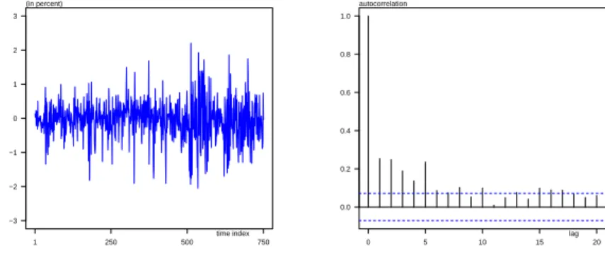
We apply our Bayesian estimation to daily observations of the Deutschmark vs British Pound foreign exchange log-returns. The sample period is from January 3, 1985, to December 31, 1991, for a total of 1974 observations. The nominal returns are expressed in percent. This data set has been promoted as an informal benchmark for GARCH time series software validation and is available from the Journal of Business and Economic Statistics (JBES). From this time series, the first 750 observations, which is somewhat less than three financial years, are used to illustrate the Bayesian approach. The number of data is large enough to perform classical Maximum Likelihood (ML) estimation and apply asymptotic justifications. Hence, we have an interesting point of view from which to compare classical and Bayesian approaches.
The observation window excerpt from our data set is plotted on the left-hand side of Figure 1. We test for autocorrelation in the times series by testing the joint nullity of autoregression coefficients for{yt}. We estimate the regression with autoregression
Thep-valueof the Wald test is 0.377 which does not support the presence of autocorre-lation. However, from Figure 1 we clearly observe clusters of high and low variability in the time series. This phenomenon is well known in financial data and is referred to as volatility clustering. This effect is emphasized on the right-hand side of Figure 1 where the sample autocorrelogram of squared observations is displayed. In this case, the first autocorrelations are large and significant, indicating GARCH effects; the Wald test strongly rejects absence of autocorrelation in the squares. As an additional data
1 250 500 750 −3 −2 −1 0 1 2 3 daily log−returns (in percent) time index 0 5 10 15 20 0.0 0.2 0.4 0.6 0.8 1.0 sample autocorrelation lag
Figure 1:Daily log-returns (left) and sample autocorrelogram (right)
analysis, we test for unit root using the Phillips and Perron [10] test. The test strongly rejects theI(1)hypothesis. From this preliminary analysis, we conclude that the time series is not integrated and does not exhibit autocorrelation. However, we strongly suspect the presence of GARCH effects in the data.
4.1
Model estimation
We fit the parsimonious GARCH(1,1) model to the data for this observation win-dow. As a prior distribution for the Bayesian estimation we choose a truncated tri-dimensional Normal distribution with a zero mean vector and a diagonal covariance matrix. The variances are set to 10’000 so we do not introduce tight prior information into our estimation. We run two chains for 10’000 passes each. We emphasize the fact that only positivity constraints are implemented in the M-H algorithm; no stationarity conditions are imposed in the simulation process.
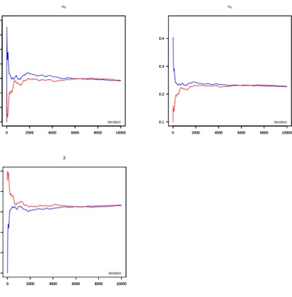
In Figure 2, the running mean is plotted over iterations. For all parameters, we no-tice a convergence of the two chains toward a constant value after something like 5’000 iterations. The diagnostic test by Gelman and Rubin [5] does not reject convergence of the chain after 5’000 passes (values ranging from 1.04 to 1.05 for the 97.5th percentile of the potential scale reduction factor). The one lag autocorrelations in the chains range from 0.75 forα1to 0.95 forβ which is reasonable. The sampling algorithm allows to
reach very high acceptance rates ranging from 89% forαto 95% forβ. From the over-all MCMC output, we discard the first 5’000 draws as aburn inperiod and merge the
two chains to get a final sample’s length of 10’000. In addition, we estimate the model by the usual Maximum Likelihood technique for comparison purposes.
0 2000 4000 6000 8000 10000 0.02 0.03 0.04 0.05 0.06 0.07 0.08 0.09 0 2000 4000 6000 8000 10000 0.02 0.03 0.04 0.05 0.06 0.07 0.08 0.09 α0 iteration 0 2000 4000 6000 8000 10000 0.1 0.2 0.3 0.4 0 2000 4000 6000 8000 10000 0.1 0.2 0.3 0.4 α1 iteration 0 2000 4000 6000 8000 10000 0.3 0.4 0.5 0.6 0.7 0.8 0 2000 4000 6000 8000 10000 0.3 0.4 0.5 0.6 0.7 0.8 β iteration
Figure 2:Running means of the chains over iterations (up to 10’000). The sampler generatesαandβfrom the candidate distribution derived in Section 3. The acceptance rate ranges from 89% forαto 95% forβ. The autocorrelations range from 0.75 for
α1to 0.95 forβ. The convergence diagnostic indicates convergence of the chains from iteration 5’000. The 97.5th percentile of the potential shrink factor ranges from 1.04 to 1.05.
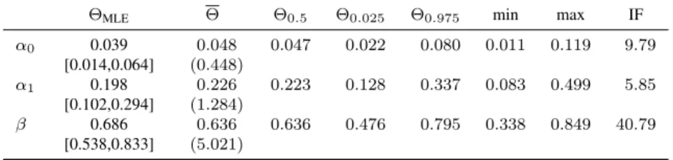
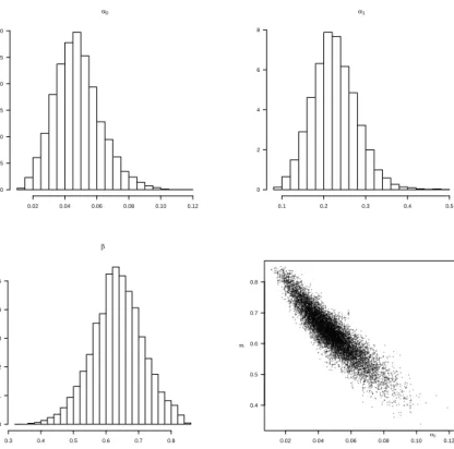
The posterior statistics as well as the ML results are presented in Table 1. First, we note that even if the number of observations is large, the ML estimates and the Bayesian posterior means are different; the ML estimation is lower forαand higher forβ. We also notice a difference between the 95% confidence intervals. Whereas the confidence band is symmetric in the ML case due to the asymptotic Normality assumption, this is not true for the posterior confidence intervals. The reason can be explained trough Figure 3 where the posterior distributions for the parameters are displayed. Indeed, we clearly notice the asymmetric shape of the histograms forα0 andα1. The skewness
values are 0.46 and 0.39, both significantly different from zero. Therefore the ML con-fidence band has a tendency to underestimate the right boundary of the 95% concon-fidence interval for these parameters. In the case ofβ, the skewness is -0.09, also significant; in this case, the Maximum Likelihood overestimate the left boundary of the 95% con-fidence band. Furthermore, as shown in the bottom right-hand side of Figure 3, the joint distribution for the parametersα0andβ is slightly different from the ellipsoid
ΘMLE Θ Θ0.5 Θ0.025 Θ0.975 min max IF α0 0.039 0.048 0.047 0.022 0.080 0.011 0.119 9.79 [0.014,0.064] (0.448) α1 0.198 0.226 0.223 0.128 0.337 0.083 0.499 5.85 [0.102,0.294] (1.284) β 0.686 0.636 0.636 0.476 0.795 0.338 0.849 40.79 [0.538,0.833] (5.021)
Table 1:Estimation results for the GARCH(1,1) model. ΘMLE: Maximum
Likeli-hood estimate.Θ: posterior mean.Θφ: estimated posterior quantile at probabilityφ.
IF: inefficiency factor (ratio of the variance of mean relative to aiidsequence).[•]: Maximum Likelihood 95% confidence interval.(•): numerical standard error (×103).
we should obtain under the multivariate Normal assumption. Therefore, these results warn us against the abusive use of asymptotic justifications; in the present case, even 750 observations do not suffice to assume the asymptotic Normal distribution for the parameters.
Finally, the last column of Table 1 gives the inefficiency factors for the different parameters. Their values are computed as the ratio of the squared numerical standard error of the MCMC simulations and the variance estimate divided by the number of iterations (i.e. the variance of the sample mean from a hypotheticaliidsampler). The numerical standard errors are estimated by the method of Andrews [1], using a Parzen kernel and AR(1) pre-whitening as presented in Andrews and Monahan [2]. This en-sures easy, optimal, and automatic bandwidth selection. Using 10’000 simulations out of the posterior distribution seems appropriate if we require that the Monte Carlo er-ror in estimating the mean is smaller than one percentage of the variation of the erer-ror due to the data. The larger inefficiency factor reported forβ is reflected in a larger autocorrelation in the simulated values.
4.2
Sensitivity analysis
The Bayesian approach is often criticized by the fact that the prior distribution for the parameters can have a significant impact to the posterior distribution, and as a consequence, bias the results. It is therefore important to determine the extend of this impact trough a sensitivity analysis. As noted by Geweke [6, Section 2], it is possible to approximate the Bayes factor between two models differing only by their prior densities using the posterior simulation output from just one of the models. This approach provides an attractive way of performing sensitivity analysis since it does not require the estimation of the alternative model.
We test the sensitivity by considering four alternative prior distributions; either by modifying the mean or/and increasing the variances relative to our initial prior. The Bayes factors are then estimated as explained in the previous paragraph and ranked with the Jeffrey’s scale of evidence. In all cases, we conclude to a weak evidence for our initial specification relative to the alternative prior, indicating that our initial prior is vague enough. The results are not shown to save space but can be obtained from the author upon request.
α0 0.02 0.04 0.06 0.08 0.10 0.12 0 5 10 15 20 25 30 α1 0.1 0.2 0.3 0.4 0.5 0 2 4 6 8 β 0.3 0.4 0.5 0.6 0.7 0.8 0 1 2 3 4 5 + + + + + + +++ + + + + + + + + + + + + + + + + + + + + + + + + + + + + + + + + + + + + + + + + + + + + + + + + ++ + + + + + + + + + + + + + + + ++ + + + + + ++ + + + + ++ + + + + + + + + + + + + + + + + + + + + + + + + + ++ + + + + + + + + + + + + + + + + + + + + + + + + + + ++ + + + + + + + + + ++ + + ++ +++ + + + + + + + + + + + + + + + + + + ++ + + + + + + + + + + + + + + + + + + + + + + + + + ++ + + + ++ + ++ + + + + + + + + + + + + + + + + + + + + + + + + + + + + + + + + + + + + + + + + + + + + + ++ + + + ++ + + + + ++ + + + + + + + + ++ ++ + + + + + + + + + + + + + + + ++ + +++ + + + +++ + + + ++ + + + ++ + + + + + + + + + ++ + + + + + + + + ++ + + + + + + + + + + + ++ + ++ + + + + + + + + + + + + + + + + + + + + + + + + + + + + + + + + + + + + + + + + + + + + + + + + + + + ++ + ++ + + + + + + + + + + + + + + + + + + + + + + + + + + + + + ++ + + + + + ++ + + + + + + + + + + + + + + + +++ + + + + + + + + + + + + + + + + + ++ + ++ ++ + + + + + + + + + + + + + + + + ++ + + + + + + + + + ++ + + + + + + + + + + + + + ++++ + + + + + + + + + + + + + + + + + + + + + + + + + + + + ++ + + + + + + + + + + + + + + + + + + + + + + + + ++ + + + + + + + + + + + + + + + + + + + + + + + + + + + + + + + + + + + + + + + + + + + ++ + + + + + + + + + + + + + + + + + + ++ + + + + ++ + ++ + + + + + + ++ + + + + + + + + ++ + + + + + + + + + + + + + + + + + + + + + ++ + + + + + + ++ ++ + + + ++ + ++ + + + + + ++ + + + + + + + + + + + ++ + + + + + + + + + + + + + + + + + + + ++ + + + + ++ + + + + + + + + + + + + + + + + + + + + + ++ + + + + + ++ + + + + + + + + + + + + + + ++ + + + + + + + + + + + + + + + ++ + + + + + + + + + + + + + + + + + + + + + + + + + + + + + + + + + + + + + + + + + + + + + + + + + + + + + + + + + + + + + + + + + + + + + + ++ + + + + + + + + + + + + + + + + + + + + + ++ + ++ + + ++ + + + + + + + + ++ ++ ++ + + ++ + + + + + + ++ + + + + + + + + + + + + + + ++ + + + + + + + + + ++ + + + + + + + + + + + + + + + ++ + + + + + + + + + + + + + + + + + + + + + + + + + + + + + + + + + + + ++ + + + + + + + + + + +++ + + + + + + + + + + + + + + + + + ++ + + + + + + + + + + + + + + + + + + + + + + + ++ + + + + ++ + + + ++ + + + + + + + + + + + + + + + + + + + + + + + + + + ++ + + + + + + + + + + + + + + + + + + + ++ + + + + + + + + + + + + + + + + + + + ++ + + + + + + + + + + + + + + + + + + + + + + + + + + + + + + + + + + ++ + + + ++ + + + + + + + + + + + + + + + + + + + + + + ++ + + + + + + + + + + + + + + + + + + + + + + + + + + + + + + + + + + + + + + + + + + + ++ + + + + + ++ + + + + + + + + + + + + + + + + + ++ + ++ + + +++ + + ++ + + + + + + + + + + + + + + ++ + +++ + + + ++ + + + + + + + + + + + + + + + + + + + + + + + ++ + + + + ++ + + + + + + + + ++ + + + + + + + ++ + + + + + + + + + ++ + + + + + + + + + ++ ++ + ++ + + + + + + + + + ++ + + + + + + + + + + + + + + + + + + + + + + + + + + + + + + + + + + + + + + + + ++ + + + + + + + + + ++ + + + + + + + + ++ + + + ++ + + + + + ++ ++ + + + + + + + + + + + + + + + + + + ++ + + + + + + + + + ++ + + + ++ + + + + + + + +++ + + + + + ++ ++ + + + + + + + + + + + + + + + + + + + + + + + + + + + + + + + + + + + + + + + + + + + + + + + + + + + + + ++ + + + + + + + + + + + + + + + + + + + + + + + + + + + + + + + + + + + + + + + + + ++ + + + + + + + + ++ + + + + + + + + + + + + + + + ++ + + + + + + + + + + + + + + +++ + + ++ + + + + + + + + + + + + + + + + + ++ + + + + + + + + + + + + + + + + + + + ++ + + + + + + + + + + + + + + + + + + + ++ + + + + + + + + + + + + + + + + + + + + + ++ + + + + + + + + + + + + + + + + + + + + + + + + + + + + + + + ++ + + + + + + + + + + + + + + + + + + + + + + + + + + + + + + + + + + + ++ + + + + ++ + + ++ + ++ + + + + + + + + ++ ++ ++ ++ + + + + + + ++ + + + + + + + ++++ + + + + + + + + + + ++ + + + + + + + + + ++ ++ + ++ + + + + + + + + + + + + + ++++ + + + + ++ + + ++ + +++ + + + ++ +++ + + + + + + + + + + + + + + + + + + + + + + + + + + + + + + + + + + + + + + + + + + + + + + + ++ + + + + + + + + + + + + + + + + + + + + ++ + + + + + + + + + ++ + + + + + + + + + + + + + + + + + + + + + + + + + + + + + + + + + + + + + +++ +++ + + + + + + + + + ++ + + + + + + + + + + + + + + + + + + + + + + + ++ + + + + + + + ++ + + + + + ++ + + + + + + + + + + + + + + + + + + + + + + + + ++ + + ++ + + + + + + + + + + + + + + + + + + + + + + + + + + + + + ++ + + + + + + + + + + + + ++ ++ + + + ++ ++ + + + + + + + + + + + + + + + + + + + + + + + + + + + + + + + + + + + + + + + + + + + + + + + + + + + + + + + + + + + +++ + + + + + + + + + + + + + ++ + + + + + + ++ + + + + + ++ + + + + + + + + + + + + + + + + + + + + + + + + + ++ + + + + + + + + + + + + + + + ++ + + + + + + + + + + + + + + + + + + + + + + + + + + + + + + + + + + + + + + + + + + + + + + + + + + ++ + + + + ++ + + + + + + + + ++ + + + + + + + + + + + + + + + + + + + ++ + + + + + + + + + + + + + ++ + + ++ ++ + + + + +++ + + + + + + + + + + + + + + + + + + ++ + + + + + + + + + + + ++ ++ +++ ++ + + + + + + + + ++ + + + + + + + + + + + + + + + + + + + + + + + + + + + + + + + + + + + + + + + + + ++ + + + + + + + + + + + + + + + + + + ++ + + + + ++++ + + ++ + + + + + + + + + + + + + + + + + + + ++ + + + + +++ + + + + + + + + + + + + + + + + + + + + + + + + + + + + + + + + + + + + + + + + + + + + + ++ + + ++ + + + ++ + + + + ++ ++ + + + ++ + ++ + + + + + + + + + + + + + + + + + + + ++ + + + ++ + + + + + + + + + + + + + + + + + + + + + + + + + + + ++ + + + + + + ++ + + + + ++ + + + + + + + + + + + + + + + + + + + + + ++ + + + + + + + + + + + + ++ + + + + + ++ + + + + ++ + + + + + + + + + + + + + + + + + + + + + + + + + ++ + + + + + + + + + + + + + + + + + + + +++ + + + + + + + + + + + + + ++ + + + +++ + + + + + + +++ ++ + + + + + + + +++ + + ++ + + + + + + + + + + + + + + + + + + + + + + + + + + + + + + + + + + + + + + + + + + + + + ++++ + + + + + + + + + + + + ++ + + + + + + + + + + + + + + + + + + + + + + + + + + + + + + + + + + ++ + + + + + + + + + + + + + + + ++ + + + + + + + + + + + + + + + + + + + + + + + + + + + + + + + + + + + + + + + + + + + + + + + + + + + + + + + + + + + + + + + + + + + + + + + + + + + + + + + + ++ + + + + + + ++ + + + + + + + + + + + + + + + + + + ++ + ++ + + + + ++ ++ + ++ + + + + ++ + + + + + + + + + ++ + + + + + + + + + + + + + + + + + + + ++ ++ + + + + + + + + ++ + + + + + + + + + + + + + + + + + + + + + + + + + + + + ++ + + + + + + + + + + + + + + + + + + + + + + + + + + + + + + + + + + + + + + + + + + + + + + + + ++ + + + + + + + + + + + + + + + + + + + + + + + + + + + + ++ + + + + + + + ++ + + + + ++ + + + + + ++ + + + + + + + + + + + + + + + + + + + + + + + + + + + + + + + + + + + + ++ + + + + + + + + + + + + + + + + ++ + + + + + + + ++ + + + + + + + + + ++ + + + + + + + ++ + + + ++ + + + + + + + ++ + + ++ + + + + + ++ + ++ + + + + + + + + + + + + + + + + ++ + + + + + + + + + + + + + + + ++ + + + + + + + + + +++ + +++ + + + + + + ++ + + ++ + + + + + + + + + + + + + ++ + + + ++ + ++ +++ + + + + + + + + + + + + + + + + + + + + + + + + + ++ + + + +++ + + + ++ + + + + + + ++ + + + + + + + + + + + ++ + + + + + + ++ + + + + + + + + + + + + + + + + + + ++ + + + + + + + + + + + + + + + + + + + + + + + + ++ + + + + + + + + + + + + + ++ + ++ + ++ + + + + + + + + + + + + + + + + + + + + ++ + + + + + + + + + + + ++ + + + + + + + ++ + + + + + + + + + ++ + + + + + + + + + + + + + + + + + + + + + + +++ + + + + + + + + + + + + ++ + + + + + + + + + + + + + + + + + + + ++ + + + + + + + + + + + + + + + + + + + + + + + + + + + + + + + + + ++ + + + + + + + + + + + + + ++ + + ++ + + + ++ + + + + + + + + + + + + + + + + + + ++ + ++ + + + + + + + ++ + + + + + + + ++ + + + + ++ + + + + + + + + + + + + + + + + + + + + + ++ + + + ++ ++ ++ + + + + + + + + + +++ ++ + + + + + + + + + + + + + + ++ + + + + + + + + + + ++ + + + ++ ++ + + + + + + + ++ ++ + + + + + + + ++ + + + + + ++ + + + + + + + + + + +++ + ++ + + + + + + + + + ++ + + ++ + + + + + + + + + + + + + + + + + + + + + + ++ + + + + + + + + + + + + + + + + + + + ++ + ++ ++ ++ +++++ ++ + + + + + + + + + + + + ++ + + + + + + +++ + + + + + + + + + + + + + + +++ + + + + + ++ + + + + + + + + + + ++ + + + + + + + + + + + + + + + + + + + + ++ + + + + + ++ + + + + + + + + + + + + + + + + + + + ++ + ++ + + + + + + + + + + + + + + + + + + + ++ + + ++ + + + + + + + + + + + + + + + + ++ + + + + + + + + + + + + + + + + + + + + + + + + + + + + ++ + + + + + + + + + + + + + + + + + + + + + + + + + + + + + + + + + + + + + + + + + + + + + + + + + + + + + + + + + + + + + + + + + + + + + + + + ++ + + + + ++ ++ + + + + + + + + + + + + + + + + + + + + + + + + + + + + + + + + + ++ + + + + + + + + + + ++ + ++ + + + + + + + + + +++ + + + + + + + + + + +++ + + + + + + + + + + ++ + + + + ++ + + + + + + + + + +++ + + + ++ + + + + + + + + + + + + + + + + + + + + + + + + + + + + + + + + ++ + + + ++ + + + + + + + + + + + + + + + + + + + ++ + + + + + + + + + + + + + + + + + + + + + ++ + + + + + + + + + + + + + + + ++ + + + + + + + + + + + + + + ++ + + + + + ++ + + + + + + + + + + ++ + + + + + + + + + + ++ + + ++ + + + + + + + + + + + + + + ++ + + + + + + + + + + + + + ++ +++ + + + + ++ ++ + + + + + + + + + + ++ + + ++ ++ + + ++ + + + + ++ + ++ + + + + + + + + + + + + + + + + + + + + + + + + + + + + + + + + + + ++ + + + + + + + + + + + + + + + ++ + +++ + + + +++ + + + ++ + + + + + + ++++ + + + + + + + + + + + + + + + + ++ ++ + + + + ++ + + + + + + + + + + + + + + + + + + + + + + + + + + + + + + + + + + + + + + + + + + + ++ + + + + + + + + + + + + + + + + + + ++ + + + + + + + + + + + + + + + + + + + + + + + + + + + + + + + + + + + + + + + + + + +++ + + + + + + ++ + + + + ++ ++ + + ++ ++ + ++ + + + + + + + + + + + ++ + + + + +++ + + + + + + + + + + + + + + + + + + + + + + + + + + + + + + + + + + + + ++ + ++ ++ ++ + + + + + + + + + + + + + + + + + + + + + + + + + + + + + + + + + ++ + + + + + + + + + + + + + + ++ + + + + + + ++ + + + + + + ++ + + + + + + + + + + + + + + + + + + + + + + + + + + + + + + + ++ + + + + + + + + + + + + + + + + + + + + + + + + + + + + + + + + + + + + + + + + + + + + + + + ++ ++ + + + + + + + + + + + + + + + + + ++ + + + + + + + + + + + + + + ++ + + + + + + + + + + + + + + + + + ++ + + + ++ + + + + + ++ + + + + + + + + + + + + + ++++ + + ++ + + + + ++ + + + + + + + + + + + + ++ + + + + + + + + + + + + ++ + + + + + + + + ++ + + + ++ + + + + + + + + + + + + + + + + + + + + + + + + + + + + + + + + + ++ + + ++ +++ + + + + + + ++ + + + + + + ++ + + + + + + + + + + + ++ + + + + + + + + + + + + ++ + + + + + + + + + + + + + + + + + + + + + + + + + + + + + + + + + + + + + + + + + + + + + + + ++ + + ++ + + + + + + + + + + + + + + + + + + + ++ + + + + + + + ++ ++++++ + + + + + + + + + + + + + + + + + + + + + + + + + + + + + + + + + + + + ++ + + ++ + + + + + + + + + + + + + + + + + + + + + + + + + + + + ++ + + + + + + ++ + + + + + + + + + + + + + + + + + + + + + + + + + + + + + + + + + + + + + + + + + + + ++ + + + + + + ++ + + + + + + + + + + + + + + + + + + + + + + + ++ + + + + + + + + + + + + + + + + + + + + + + + + + + + + + + + + + + + + + ++ + + + + + + + + ++ + + + + + + + + + + + + + + + + + + + + + + + + + + + + + + + ++ + + + + + + + + + + + + + + + + + + ++ + + + + + + + + + + + + + + + + + + + + + + + + + + + + + + + ++ + + + + + + + + + + + ++ + + + + + + + + ++ + +++ + + + + + + + + + + + + + + + + + + + + + + ++ ++ + + ++ + + + + + ++ + + + + + + ++ ++ + + + + + + + + + + + ++ + + + + ++ ++ + + + + ++ + ++ + + + + + + + + + + + + ++ + + + + + + + + + + + + + ++ + + + + + + + + + + ++ + + + + + + + ++ + + + + + + + + + + + + + + + + + + + + + + + + + + + + + + + + + + + ++ + + + + + + + + + + + + + + + + + + + + + + + + + ++ + + + ++ + + + + + + + ++ + + + ++ + + + + + + ++ + + + + + + + ++ + + + + ++ + + + + + + + + + + + + + + + + + + + + +++ + + ++ + + + + + + + + + + ++ + + + + + + + + + + + + + + + + + + + + + + + + + + + + + + + + + + + + + + + + + + + + + + + + + + ++ + + + + + + + + ++ + + + ++ + + + + + ++ + + + + + + + + + + + + + + + ++ + + + + + + ++ + + + + + + ++ + + + + + + + + + + + + + + + + + + + + ++ + + + + + + + + ++ + + ++ + + + + + + + ++ + + ++ + + + ++ + + + + + + + + + + + + + + + + + + + + + + + + + + + + + ++ + + + + + + + + + + + + + ++ + + + + + ++ + + + + + + + ++ + + + ++ + + + + + + +++ + + + + + + + + + + + + + + ++ + + + +++ + + ++ + + + + + ++ +++ + + + + + + + + + + ++ + + + + + + + + + + ++++ ++ + + + + + + + + + + + + + ++ + + + + + + ++ + + + + ++ + + + + + + + + + + + + + + + + + + + ++ + + + + + + + + + + + + ++ + + + + + + + + ++ + + + + ++ + + + + + + + + + + + + + + + + + + + + + + + + + + + + + + + + + + + + + + + + + + + + + + + + + + + + + + + + + + + + + ++ + + + + + + + + + + + + + + + + + + + + + + + + + + + + + + + + + + + + + + + + + + + + + + + + + + + + + + + + + + + + + + + + ++ + + + + + + + + ++ + + ++ + + + + + + + + + + + + + + + + + + + + + + + + + + + + + + + ++ + + + + + + + + + + + + + + ++ + + + + + + + + ++ + + + + + + + ++ + + + + + + ++++ + + + + + + + ++ + + ++ + + + ++ + + + + + + + + + + + + + + ++ ++ ++ + + + + + + + + + + + + + + + + + + + + + + ++ + + + + + + + + + + + + + + + + + + + + + + + + + + + + + + + + + + + + + + ++ + + + + + + + + + + + + + + + + + + + + + + + + + ++ + + + + + + + + + + + + + + + + + + + + + + + + + + + + + + + + + + + + + + + + + + + + + + + + + + + + + + + + + + + + + + + + + + + + + + + ++ + + + + + + + + + + + + + +++ + + + + ++++ ++ + + + + + + + + + + + + + + + + + + + + ++ + + + + ++ + + + + + + + + + ++ + + + ++ ++ + + + + + + + + + + + + + + + + + + + + + + + + + + + + + + + + + + + ++ + + + + + + + + + ++ + + + + + ++ + + + + + + + + + + + + + + + + + + + + + + + + + + ++ + + + + + + + + + + + + + + + + + + + + + + + + + + ++ + + + + + + + + + + + + + + + + + + + + + + ++ ++ + + + + + + + + + + + + + + + + + + + + + ++ + + + + + + + + + ++ + + + ++ + + + + ++ + + + + + + + + + + + ++ + + ++ + + + + + + + + + + + + + + + + + + + + + + ++ + + + + + + + + + + + + + + ++ + + + + + + + + + + + + + + ++ + + + + + + + + + + + + + + + + + + + + + ++ + + + + + + + + + + ++ + + + ++ + + + + + + + + + + + + + + + + + + + + ++ + ++ + + + + + + + + + + + + + + + + + + + + + + ++ + + + + + + + + + + + + +++++ ++ + + + + + + + + + + + + + + ++ + + + + + + + + + + + + + + + + + + + + + + + + + + + + + + + + + + + + + + + + + + + + + + + + + + + + + + + + ++ + + + + + + + ++ + + + + + + + + + + + + + + + + + + + + + + + + + + + + + + + + + + + + + + + + + + + + + + + + + + + + + + + + + + + + + ++ + + + + + + + + + + + + + + + + + ++ + + + + + + + + + + + + + + + + + + + ++ + + + + + + + + + + + + + + + + + + + + + + + ++ + + + + + + + + + + + + + ++ + ++ + + + + + + + + + + + + + + + + + + + + + + + + + + + + ++ + + + + + + + + + + + + + + + + + + + + + + + + + + ++ + + + ++ ++ + + + + + + + + + + + ++ + + + + + ++ + ++ + + + ++ + + + + + + + + + + + + ++ + + + + + + + + + + + + + + + ++ + + + + + + + + + + + + + + + + +++++ ++++ + + + + ++ + ++ + + + + + + + + ++ + + + + + + + +++ + + + + + + + + + + + + + + + + + + + + ++ + + + + + + + + + + + + + + + ++ + + + + + + + + + + + + ++ + + + + + + ++ + + + + + + + + + +++ + + + + + + + + + + + + + + + + + ++ + + + + + + ++ + + + + + + + + + + + + + + + + + + ++ + ++ + ++ + + + + + ++ + + + + + + + + + + + + + + + + + + + + + + ++ + + + + + + + + + + + + + + + + + + + + + + + + + +++ + + + + + + + + + + + + + + + + ++ + + + + + + + + + ++ ++ + ++ + + + + + + + + + + + + + + + + + + ++ + + + + + + + + + + + + + + + + +++ + + + + + + + + + + + + + + + + + + + + + + + + ++ + + + + + + + ++ + + + + + + + + + + + ++ + + + + + + + + + + + + + + + + + + + + + + + + + + + + + + + + + + + + + + + + + + + + + + + + + + + + + + + + + + + + + + + + + + + + + ++ + + + + + + + + ++ + + + + + ++ + + + + + + + + + + + + + + +++++ + + +++ + + + + + ++ + + + + ++++ + + + + + + + + + + + + + + + + + + + + + ++ + + + + + + + + + + + + + + + + ++ + + + + + + + + + ++ ++ + + + + + + + + + + + + + + + + + + + + + + + + + + + + + ++ + + + ++ + + + + + + + ++ + + + + + + + + ++ + + + + + + + + + + + + + + + + + + + + + + + + + + + + + + + + + + + + + + +++ + + + + + + + + ++ + + + + + + + + ++ + +++ + + + + + + + ++ + + + + + + + + + + + + + ++ + + + + + + + ++ ++ + + +++ + + + + ++ + + + + + + ++ + + + ++ + + + + + + + + + + + + + + + + + + +++ + + + + + + + + + + + + + + + + + + + + + + + + + ++ + + + + + + + + + + + + + + + + + + + + + + + + + + ++ + + + ++ + + + + + + + + + + + + + + + + + + ++ + + + + + + + + + + + + + + + + + + + + + + + + + + + + + + + + + + + + + + + + + + + + + + + + + + + + + + + + + + + +++ +++ + + ++ + + + + + ++ + + + + + + + + + + + + + + + +++ ++ + +++ + ++ + +++ + + + + +++ + + + + + + + ++ + + + + + + + + ++ + + + + + + ++ + + + + + + + + + + + + + + + + + + + + + + + ++ + ++ + + + + + + + + + ++ + + + + + + + + + ++ + + + + + +++ + + + + + + + + + + + + + + + +++ + + + + + + + + + + + ++ + + + + + + + + + + + + + + + + + ++ + + + + + + + + + + + + ++ + + ++ + + + + + + + + + + + + + + + + ++ + + + + + + + + + + + + + + + + + + + + + + + + + + + + ++ + + + + + + ++ + + + + + + + + + + + ++ + + + + + + + + + + + + + + + + + ++ + + +++ + + + + + + + + + + + + + + + + + + + + + ++ + + + + + + + + + + + + + + ++ + + + + + + + + + + + + + + ++ ++ + + + +++ + + + + + + + + + + + + + + + + + + + + + + + + + + + + + + + ++ + + + + + + + + + + + + ++ + + + ++ + + + + + + + + + + + + + + + + + + + + + + + + + + + ++ + + + + + + + + + + + + + + + + + + + + + + + + + + + + + + + + + + + + + + + + + + + + + + + + + + + + + + + + + ++ + + + + + + + + + + + + + + + + + + + + + + + + + + + ++ + + + + + + + + + + + + ++ + + + + + + + + + + + + + + + + + + + + + + + + + + + + + + ++ + + + + + + + + + + + + + + + ++ ++ + + + + + + + + + + + + + + + + + + + ++ + + + + + ++ + + + + + + + + + + ++ + + + + + + +++ + + + + + + + + + + + + + + + + + + + + + + + + + + + + + + + + + + ++ + + + + + + + + + + + + + + + + + + + + + + + + + + + + + + + + + + + + + + + + + ++ + + + + + + + + + + + + + + + + + + + + + + + + + ++ + +++ + + + + + ++ + + + ++ + + + + + + + + ++ + + + + + + + +++ + + + ++ ++ + + + + + + + + + + + + + + ++ + + + + ++ + + + + + + + + + + + + ++ + +++ + + ++ + + + + +++ +++ ++ ++ + + ++ + + + + + + ++ ++ + ++ + + + + ++ + + + ++ + + + + + + ++ + + + + + + + + + + + + + + + + + ++ ++ + +++ + + + + ++++++ + + + ++ + + + + ++ + + + + + + + + + + ++ + + + + + + + + + + + + + + ++ + + + + + + + + + + + + + + + ++ + + + ++ + + + + + + + + + + + + + + + + + + + + + + ++ + + + + + ++ ++ + + + + + + + + + + + + + + + + ++ + + ++ + + + + + + ++ + + + + + + + + + + + + ++ + + + + + ++ + + + ++ + + + + + + + + + + + + + + + + + + + + + + + + + + + + + + + + + + + + + + + + + + + ++ + ++ + + ++ + + + + ++ + + ++ + + + + + + + + + + + + + + ++ + + + + + + + + + + + + + + + ++ + ++ + + + + + + + + + + + + + + + + + + + + + + + + + + + + + + + + + + +++ + + + + + + + + + + + + + + + + + + + + + + + + + + + + + + + + + ++ + + + + + + + + + + + + + + + + + + ++ + + + +++ + + ++ + + + + ++ + + + + + + + + + + + + + + + + + + + + + + + + + + + + + + + + + + + + + + + + + + + + + + + + + + + + + ++ + + + + ++ ++ ++ + + + + + + + + + + + + + + + + + + ++ + + + + ++ + ++ + + + + + + + + + + + + + + + ++ + + + + + + + + +++ + + + + + + + + + + + + + ++ + + + + + + + + + + + + + + + + + + + + + + ++ + 0.02 0.04 0.06 0.08 0.10 0.12 0.4 0.5 0.6 0.7 0.8 β α0
Figure 3:Posterior distributions for the GARCH(1,1) parameters based on 10’000 draws. In the lower-right graphic, we present a scatter plot of posterior(α0, β)
4.3
Model diagnostic
We check for model misspecification by testing the standardized residuals.1 They are
defined by:
b
εt:=ytbh −1/2
t
fort = 1, . . . ,750wherebhtis the conditional variance computed withΘ0.5(the
me-dian of the posterior sample). If the statistical assumptions in (2.1) are satisfied, these residuals should be independent and Normally distributed.
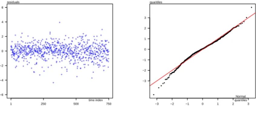
On the left-hand side of Figure 4 we display the residuals over time. No autocor-relation or heteroscedasticity are visually apparent. We test for autocorautocor-relation using the Ljung-Box test up to lag 20. The test does not reject the null at the 5% level (p -value= 0.652). This is also true for the squared residuals (p-value= 0.961). Hence, the GARCH(1,1) process has been able tofilterthe heteroscedastic nature of the data. We form a quantile-quantile plot of the residuals against the Normal distribution on the right-hand side of Figure 4. The distribution is almost Normal at its center whereas the tails are slightly fatter, especially the left one. The Kolmogorov-Smirnov Normality
1An alternative would be to test the predictive performance of the model over an out-of-the-sample
win-dow (i.e. specification test). This approach is however not pursued in this article since we consider a single model and we focus on the estimation instead of the forecasting performance. A misspecification test is simpler and certainly sufficient in this context.
test rejects the null hypothesis at the 5% level (p-value= 0.008). The tails of the in-novations’ distribution are not fat enough to fully capture the distributional nature of the data. This point is recurrent with financial data and heavy tails distributions for the innovations are sometimes useful to overcome this problem.
+ ++ + + + + + + + +++ + + +++ + + + + + + + + + + + + + + + + + + + + ++ + + + + + + + + + + + + + + + + + + + + + + + + + + + + + + + ++ + + ++ + + + + + + + + + + + + + + + + + + + + + + + + + + + + + + + ++ + + + + + + + ++ + + + ++ + + + + + + + + + + + ++ + + + + + + + + ++++ + + + + + + + + + + + + + + + + + + + ++ + + + ++ + + + + + + + + + + + ++++ + ++ + + + ++ + + + + + + + ++ + + + + + + + ++ + + + ++ + + + + + + + +++ + + + + + + + + + + + + + + + + ++ + + + + + + + + + + + + ++ + + ++ + + + ++ + + + + + + + + + + + + + + + + + + + + + + + + + + + + + + + + + + + ++ + + + +++ + ++ + + + ++ + + + + + + + + + + + + + + + + + + + + + ++ + + + ++ + + ++ + + + + + + + + + + + + ++ + + + + + + + ++ + + + + + + + + + + + + + + + + + + + + + + + + + + + + + + + + + + + + + + + + + + + + + ++ + + + + + + + + + + + + +++ + + + + + + + + + + + + + + + + + + + + + + + + + + + + + + + + + + + + + + + + + + + + + + + + ++ + + + + + + + + + + + + + + + + + + + + + + + + + + + + + + ++ + + + + + + + + + + + + + + + + + + + + + + + + + + + + + + + + + + + + + + + + + + + + + + + + + + + + + + + + + + ++++ + + + + + + ++ + + + + + + + + + + + + ++ + + + + + + + + + + + + + + + + + + + + + + + + + + + + + + + + + + + + + + + + + + + + + + + + + + + + + + + + + + ++ + + + + + + + + + + + + + + + + + + + + + + + + + + + + + + + + + + + ++ + + + + + + + + + + + + +++ + + + + + + + + + + + + + + + ++ + + + + + + + + + + + + + + + −6 −4 −2 0 2 4 6 1 250 500 750 time index residuals −3 −2 −1 0 1 2 3 −3 −2 −1 0 1 2 3 Normal quantiles sample quantiles
Figure 4:Residuals (left) and quantile-quantile plot (right)
5
Illustrative applications
In this section, we illustrate some interesting probabilistic statements made possible under the Bayesian framework. The joint posterior sample is used to simulate complex functions of the parameters.
5.1
Persistence
As pointed out in Section 3, a GARCH(1,1) process for{yt}is equivalent to an ARMA(1,1)
process for{y2
t}with an autoregressive coefficient(α1+β), and a moving average
co-efficient−β. The autocorrelation function (ACF) comes from the standard formulae for the ARMA(1,1) model. It is recursively given byρi:= (α1+β)·ρi−1for(i >2)
with the first order autocorrelation given by:
ρ1:=α1
1−β2−α1β
1−β2−2α 1β
.
The term(α1+β)is the degree of persistence in the autocorrelation of the squares. It
controls the intensity of the clustering in the variance process. With a value close to one, past shocks and past variances will have a longer impact on the future conditional variance. An autoregressive coefficient(α1+β) = 1corresponds to a unit root process
for squared observations.
To make inference on persistence and ACF, we simply use the posterior sample
Θ[j]and generate(α[j]+β[j])andρ[j]
graphic of the posterior distribution of the persistence(α1+β)is plotted on the
left-hand side of Figure 5. The histogram is slightly left-skewed with a median value of 0.865 and a maximum value of 0.992. In this case, the integration for the variance process is not supported by the data. On the right-hand side of Figure 5 we display the posterior ACF with its 95% and 99% confidence bands together with the sample autocorrelations. Although a single observation (at lag 11) lies outside the confidence bands, the autocorrelation structure of the estimated GARCH(1,1) model is in line with the data. α1+ β 0.7 0.8 0.9 1.0 02468 5 10 15 20 0.0 0.2 0.4 0.6 0.8 5 10 15 20 0.0 0.2 0.4 0.6 0.8 5 10 15 20 0.0 0.2 0.4 0.6 0.8 5 10 15 20 0.0 0.2 0.4 0.6 0.8 5 10 15 20 0.0 0.2 0.4 0.6 0.8 ++ + + + + ++ + + + + ++ ++ + + ++ 5 10 15 20 0.0 0.2 0.4 0.6 0.8 theoretical and sample autocorrelations lag + median 95% confidence band 99% confidence band sample autocorrelation
Figure 5: Posterior distribution for the persistence (left) and posterior autocorrel-ogram (right). The solid line is the posterior median, the dashed lines the 95% con-fidence bands and the dotted lines the 99% concon-fidence bands. The cross symbols are values of the sample autocorrelation of the squared log-returns up to lag 20.
5.2
Stationarity
In the case of the GARCH(1,1) process, Nelson [9] gave the conditions for covariance stationarity (CSC) and strict stationarity (SSC). These conditions are given by:
CSC := α1+β−1<0
SSC := E[ln(α1ε2t+β)]<0
where the error termεtis Normally distributed. As pointed out in Section 4, the
co-variance stationary condition has not been imposed in the M-H algorithm. The joint posterior sample can be used to estimate the posterior distribution of these functions:
CSC[j] := α1[j]+β[j]−1 SSC[j] := 1 K K X k=1 ln(α[1j](η[k])2+β[j])
forj = 1, . . . ,100000, whereη[k] is a draw from a standard Normal distribution and
K is set large enough (in our application we chooseK = 10000). In Figure 6 we present the posterior distributions forCSC andSSC. None of these values exceed zero in our simulation study. The estimated model is therefore covariance stationary and strictly stationary. Other probabilistic statements on interesting functions can be
−0.5 −0.4 −0.3 −0.2 −0.1 0.0 02468 1 0 −0.5 −0.4 −0.3 −0.2 −0.1 0.0 02468 1 0 covariance stationarity strict stationarity
Figure 6: CSCandSSCposterior distributions. Gaussian kernel density estimates with bandwidth selected by the ’Silver-man’s rule of thumb’ criterion (Silverman [11, page 48]).
obtained using the joint posterior sample. For example, the posterior median is 0.341 for the marginal variance and 4.54 for the marginal kurtosis. They approximately cor-respond to the sample estimations of 0.323 and 4.63.
6
Conclusion
This paper has proposed the estimation of the Bayesian GARCH(1,1) model with Nor-mal innovations. The MCMC scheme has been derived in order to simulate the joint posterior distribution for the model’s parameters. The GARCH(1,1) model has been applied to foreign exchange log-returns time series and comparison with the traditional Maximum Likelihood has been performed. It has been shown that even if the sam-ple size is fairly large (in our case 750 observations), point estimates differ slightly between the two approaches. In addition, the posterior distribution for some param-eters is skewed which warn us against the abusive use of the Normal approximation. A sensitivity analysis has been performed in order to robustify the estimation results. Finally, we have illustrated some appealing aspects of the Bayesian approach through interesting probabilistic statements made on the parameters.
As a final comment, we note that some financial models might use GARCH param-eters as input quantities. This is the case for instance with the Black-Scholes formula in options pricing, which is a function of the marginal variance of the underlying finan-cial asset. Under GARCH(1,1) dynamics, this marginal variance isα0/(1−α1−β)
if the process is covariance stationary, and this value can be simulated to obtain a full distribution. Then, the posterior distribution of the marginal variance could be used to simulate the option price’s distribution. Furthermore, subjective constraints on the parameters could be integrated in the MCMC procedure; for instance, an option trader could set prior lower or/and upper boundaries for the unconditional variance and then run the estimation process to estimate the GARCH parameters.
References
[1] D. W. K. Andrews. Heteroskedasticity and autocorrelation consistent covariance matrix estimation.Econometrica, 59(3):817–858, May 1991.
[2] D. W. K. Andrews and J. C. Monahan. An improved heteroskedasticity and au-tocorrelation consistent covariance matrix estimator. Econometrica, 60(4):953– 966, July 1992.
[3] Siddhartha Chib and Edward Greenberg. Bayes inference in regression models with ARMA(p,q) errors.Journal of Econometrics, 64:183–206, 1994.
[4] Robert F. Engle. Autoregressive conditional heteroscedasticity with estimates of the variance of United Kingdom inflation.Econometrica, 50(4):987–1008, 1982. [5] Andrew Gelman and Donald B. Rubin. Inference from iterative simulation using
multiple sequences.Statistical Science, 7(4):457–472, 1992.
[6] John F. Geweke. Simulation methods for model criticism and robustness analysis. In J. O. Berger, J. M. Bernardo, A. P. Dawid, and A. F. M. Smith, editors,Bayesian Statistics, volume 6, pages 275–299. Oxford: Oxford University Press, 1999. [7] John F. Geweke. Getting it right: Joint distribution tests of posterior
simula-tors.Journal of the American Statistical Association, 99(467):799–804, Septem-ber 2004.
[8] Teruo Nakatsuma. A markov-chain sampling algorithm for GARCH models.
Studies in Nonlinear Dynamics and Econometrics, 3(2):107–117, 1998.
[9] Daniel B. Nelson. Conditional heteroskedasticity in asset returns: A new ap-proach.Econometrica, 59(2):347–370, 1991.
[10] P. C. B. Phillips and Pierre Perron. Testing for a unit root in time series regression.
Biometrika, 75:335–346, 1988.
[11] B. W. Silverman. Density estimation for statistics and data analysis. Lon-don:Chapman and Hall, first edition, 1986.

![Figure 6: CSC and SSC posterior distributions. Gaussian kernel density estimates with bandwidth selected by the ’Silver-man’s rule of thumb’ criterion (Silverman [11, page 48]).](https://thumb-us.123doks.com/thumbv2/123dok_us/9037762.2801567/13.892.355.537.264.436/posterior-distributions-gaussian-estimates-bandwidth-selected-criterion-silverman.webp)
