Theses and Dissertations
May 2013
Three Essays on Quantile Regression
Liang Wang
University of Wisconsin-Milwaukee
Follow this and additional works at:https://dc.uwm.edu/etd
Part of theEconomics Commons
This Dissertation is brought to you for free and open access by UWM Digital Commons. It has been accepted for inclusion in Theses and Dissertations by an authorized administrator of UWM Digital Commons. For more information, please [email protected].
Recommended Citation
Wang, Liang, "Three Essays on Quantile Regression" (2013).Theses and Dissertations. 175.
by
Liang Wang
A Dissertation Submitted in Partial Fulfillment of the Requirements for the Degree of
Doctor of Philosophy in
Economics
at
The University of Wisconsin-Milwaukee May 2013
THREE ESSAYS ON QUANTILE REGRESSION
by
Liang Wang
The University of Wisconsin-Milwaukee, 2013
Under the Supervision of Professor Antonio F. Galvao
The first chapter studies identification, estimation, and inference of general uncon-ditional treatment effects models with continuous treatment under the ignorability assumption. We show identification of dose-response functions under the assump-tion that selecassump-tion to treatment is based on observables. We consider estimaassump-tion of dose-response functions through moment restriction models with generalized resid-ual functions which are possibly non-smooth, and propose a semiparametric two-step estimator. This general formulation includes average and quantile treatment effects as special cases. The asymptotic properties of the estimator are derived. We also de-velop statistical inference procedures and show the validity of a bootstrap approach to implement these methods in practice. Monte Carlo simulations demonstrate that the test statistics have good finite sample properties. Finally, we apply the proposed methods to estimate unconditional average and quantile effects of mothers’ weight gain and age on birthweight.
The second chapter develops a new minimum distance quantile regression (MD-QR) estimator for panel data models with fixed effects. We establish consistency and derive the limiting distribution of the MD-QR estimator for panels with a large number of cross-sections and time-series. The limit theory allows for both sequential and joint limits. The proposed estimator is efficient in the class of minimum distance estimators. In addition, the MD-QR estimator is computationally fast, especially
sample performance. Finally, we illustrate the use of the estimator with a simple application to the investment equation model.
The third chapter proposes tests for slope homogeneity across individuals in quan-tile regression fixed effects panel data models. The tests are based on the Swamy statistic. We establish the asymptotic null distribution of the tests under large panel data, with sequential and joint limits. Monte Carlo experiments show good perfor-mance of the proposed tests in finite samples in terms of size and power. Finally, we test and reject the hypothesis of homogeneous speed of capital structure adjustment across firms using a panel dataset.
1 Uniformly Semiparametric Efficient Estimation of Treatment
Ef-fects with a Continuous Treatment 1
1.1 Introduction . . . 1
1.1.1 Literature and Outline . . . 4
1.2 The Model, Identification, and Estimation . . . 6
1.3 Asymptotic Properties . . . 13
1.3.1 Consistency . . . 13
1.3.2 Weak Convergence . . . 17
1.3.3 Semiparametric Efficiency of the Two-Step Estimator . . . 20
1.3.4 Estimation of π0 . . . 21
1.3.5 Inference on the DRF . . . 23
1.4 Monte Carlo . . . 26
1.5 Applications to the Study of Dose-Birthweight Functions . . . 28
1.5.1 Data . . . 29
1.5.2 Estimation of Nuisance Parameter π0 . . . 32
1.5.3 Empirical Results . . . 33
1.6 Conclusion . . . 40
2 Efficient Minimum Distance Estimator for Quantile Regression Fixed Effects Panel Data 42 2.1 Introduction . . . 42
2.2 The Model and the Estimator . . . 46
2.3 Asymptotic Theory: i.i.d. within Individuals . . . 50
2.4 Asymptotic Theory: Extensions to Dependent Data . . . 55
2.5 Monte Carlo Simulations . . . 58
2.5.1 Bias and SD Results . . . 59
2.5.2 The Estimators of SD . . . 60 2.5.3 Estimation Speed . . . 62 2.6 Application . . . 66 2.6.1 Data Description . . . 70 2.6.2 Estimation Results . . . 71 2.7 Summary . . . 73
3 Testing Individual Slope Homogeneity in Quantile Regression Panel Data Models with an Application to Firm Capital Structure 75 3.1 Introduction . . . 75
3.2 The Null Hypothesis and the Proposed Tests . . . 78
3.3 Asymptotic Properties of the Tests . . . 81
3.4 Extensions to Dependent Data . . . 83
3.5 Finite Sample Simulations . . . 84 iv
3.5.2 Dynamic Model . . . 88 3.6 An Application: Target Capital Structure Adjustment . . . 95 3.7 Conclusion . . . 107
Bibliography 108
Appendix A 121
Appendix A1: Asymptotic Results for Generic Z-Estimators . . . 121 Appendix A2: Proofs of the Results in Appendix A1 . . . 126 Appendix A3: Long Proofs of the Results in Chapter 1 . . . 131
Appendix B 142
Appendix B1: Proofs of the Theorems in Chapter 2, Section 3 . . . 142 Appendix B2: Proofs of the Theorems in Chapter 2, Section 4 . . . 158
Appendix C 162
Appendix C1: Proofs of the Theorems in Chapter 3 . . . 162 Appendix C2: The Definitions of the Variables in the Dataset . . . 168
Curriculum Vitae 169
1.1 Distribution of the Months of First Prenatal Care Visit . . . 31 1.2 Mothers’ Weight Gain during Pregnancy and Level of Birthweight . . 34 1.3 Mothers’ Weight Gain during Pregnancy and Level of Birthweight
with 90% Confidence Bands . . . 35 1.4 Mothers’ Age and Level of Birthweight . . . 38 1.5 Mothers’ Age and Level of Birthweight with 90% Confidence Bands . 39 2.1 MD Estimators of the Quantile and Mean Regression . . . 72 3.1 The Histograms of ˆρi(τ) of All the Firms . . . 98
3.2 The Histograms of ˆρi(τ) of All the Firms with 0<ρˆi(τ)<0.97 . . . . 102
3.3 The Histograms of ˆρi(τ) of All the Firms with 0 <ρˆi(τ) <0.97 and
T = 31 . . . 105
1.1 Summary Statistics . . . 32 1.2 Treatment Effects of Mothers’ Weight Gain During Pregnancy . . . . 36 1.3 Treatment Effects of Mothers’ Age . . . 41 2.1 Bias and SD of the QR Estimators of the Location Shift Model When
the Innovations Are N(0,1) . . . 60 2.2 Bias and SD of the QR Estimators of the Location Shift Model When
the Innovations Are t(3) . . . 61 2.3 Bias and SD of the QR Estimators of the Location Shift Model When
the Innovations Are χ2(3) . . . 62
2.4 Bias and SD of the QR Estimators of the Location-Scale Shift Model When the Innovations Are N(0,1) . . . 63 2.5 Bias and SD of the QR Estimators of the Location-Scale Shift Model
When the Innovations Are t(3) . . . 64 2.6 Bias and SD of the QR Estimators of the Location-Scale Shift Model
When the Innovations Are χ2(3) . . . 65
2.7 Average of the Estimated SD of the Location Shift Model When the Innovations Are N(0,1) . . . 66 2.8 Average of the Estimated SD of the Location Shift Model When the
Innovations Are t(3) . . . 66 2.9 Average of the Estimated SD of the Location Shift Model When the
Innovations Are χ2(3) . . . 67
2.10 Average of the Estimated SD of the Location-Scale Shift Model When the Innovations Are N(0,1) . . . 67 2.11 Average of the Estimated SD of the Location-Scale Shift Model When
the Innovations Are t(3) . . . 68 2.12 Average of the Estimated SD of the Location-Scale Shift Model When
the Innovations Are χ2(3) . . . 68
2.13 Duration of the Estimations . . . 69 2.14 Descriptive Statistics . . . 70 3.1 Empirical Size and Power for Static Location Model withN(0,1) and
B(2,6) Innovations across Quartiles. Estimation with Nonsandwich Form and True Sparsity Function. . . 86 3.2 Empirical Size and Power for Static Location Model with N(0,1)
and B(2,6) Innovations for Median Regressions. Estimation with Nonsandwich Form and Estimated Sparsity Function. . . 87 3.3 Empirical Size and Power for Static Location and Location-Scale
Models with N(0,1) and B(2,6) Innovations across Quartiles. Es-timation with Sandwich Form and True Sparsity Function. . . 89
Estimation with Sandwich Form and Estimated Sparsity Function. . . 91 3.5 Empirical Size and Power for Dynamic Location Model with N(0,1)
and B(2,6) Innovations across Quartiles. Estimation with Nonsand-wich Form and True Sparsity Function. . . 93 3.6 Empirical Size and Power for Dynamic Location Model with N(0,1)
and B(2,6) Innovations for Median Regressions. Estimation with Nonsandwich Form and Estimated Sparsity Function. . . 94 3.7 The Summary Statistics of ˆρi(τ) for All Firms . . . 99
3.8 The Test Statistics for All the Firms . . . 100 3.9 The Summary Statistics of ˆρ(τ) for All Firms with 0<ρˆi(τ)<0.97 . 101
3.10 The Test Statistics for All the Firms with 0<ρˆi(τ)<0.97. . . 103
3.11 The Summary Statistics of ˆρi(τ) for All Firms with 0 <ρˆi(τ)<0.97
and T = 31. . . 104 3.12 The Test Statistics for All the Firms with 0<ρˆi(τ)<0.97 andT = 31.106
First, I would like to thank Dr. Antonio F. Galvao for advising me on this project.
Also, I would like to thank the committee members Dr. Scott Adams, Dr. Chuan Goh, Dr. Suyong Song, and Dr. Zhijie Xiao.
Finally, I would like to thank Dr. Ted Juhl for valuable discussions.
Chapter 1
Uniformly Semiparametric Efficient Estimation of
Treatment Effects with a Continuous Treatment
1.1
Introduction
This chapter studies identification, estimation, and inference of general uncondi-tional treatment effect (TE) models with a continuous dose of treatment. We con-sider estimating the parameters of interest, dose-response functions (DRF), through moment restriction models in which generalized residual functions are possibly non-smooth. In this general formulation, the DRF include mean and quantile functions as special cases, and consequently average treatment effects (ATE) and quantile treatment effects (QTE) are direct applications of the methods developed in this chapter.
In this chapter, the ignorability assumption is used to achieve identification of parameters of interest. The ignorability assumption states that “given a set of observed covariates, each individual is randomly assigned either to the treatment group or to the control group”; see Firpo (2007). This condition has been largely employed in TE literature, see e.g. Rubin (1977), Barnow et al. (1980), Heckman et al. (1998), Dehejia and Wahba (1999), Firpo (2007), Flores (2007), Angrist and Pischke (2009), and Cattaneo (2010) for a review.
Based on the identification condition, we construct a two-step estimation proce-dure. The implementation of the estimator in practice is simple. In the first step, one estimates a ratio of two conditional distributions, which is similar to a propen-sity score. In the second step, an optimization problem is solved. It is important
to note that, once the identification is achieved and a DRF is estimated, other pa-rameters of interest based on these functions can be estimated with little additional effort. For example, one can easily estimate TE, which are defined as differences of the DRF evaluated at different levels of treatment. In addition, one could estimate the entire curve of potential outcomes or the DRF.
Mild sufficient conditions are provided for the two-step estimator to have desired asymptotic properties, namely, consistency, weak convergence, and semiparametric efficiency. In particular, we show that the two-step estimator of a DRF is uniformly consistent over a set of treatment. Different from the binary or multi-valued treat-ment models, in which case pointwise results are equivalent to uniform results, when treatment levels are an interval T, the uniform results are stronger than pointwise results, and consequently, only pointwise results are often not adequate for infer-ences. In addition, we show that the estimator converges weakly to a Gaussian process, and that it is uniformly semiparametric efficient. For the latter derivation we use the method of Bickel et al. (1993).
Technically, the derivations of the asymptotic properties for the proposed esti-mator are independently interesting. Because the semiparametric model considered encompasses continuous treatment levels and nuisance parameters, both of which are infinit dimensional, existing results available in the literature are not directly applicable. Therefore, an additional contribution of this chapter is to provide suffi-cient conditions for consistency and weak convergence of generic moment restriction estimators (Z-estimators) with possibly non-smooth functions and a nuisance param-eter, when both the parameter of interest and the nuisance parameter are possibly infinite dimensional. These general results are used to prove the asymptotic prop-erties of the two-step estimator discussed above. In this general setting, the data need not be independent and identically distributed (i.i.d.). These results extend those of Chen et al. (2003) in that the parameter of interest is not in a Euclidean
space but in a generic Banach space. Moreover, the results extend Theorem 3.3.1 of van der Vaart and Wellner (1996) in that a possibly infinite dimensional nuisance parameter needs to be estimated in the first step. This is an important innovation because it facilitates the derivation of the limiting results for general Z-estimators, and can be utilized in future works for other statistical models.
In addition, we develop statistical inference procedures based on the two-step es-timator. In particular, we conduct inference on a DRF uniformly over the treatment levels. We propose testing procedures for the hypothesis of the equality of a DRF and any given function. The test statistics used are Kolmogorov and Cram´er-von Mises types, which detect any deviation of the null hypothesis. Since the parameter of interest is infinite dimensional and the weak limit of these statistics are not stan-dard, we compute critical values using a bootstrap method. We provide sufficient conditions under which the bootstrap is valid, and discuss an algorithm for practical implementation. The proof of the validity of the bootstrap is also an extension of that in Chen et al. (2003).
We conduct Monte Carlo simulations to evaluate finite sample performance of the test statistics. The simulations show that the Cram´er-von Mises type test statistic has good empirical size and high power against a few alternatives. In addition, the result is improved when the sample size increases, and is not sensitive to the selected numbers of bootstrap.
To illustrate the proposed methods, we consider an empirical application to a birthweight study using data from the National Vital Statistics System of Centers for Disease Control and Prevention. We estimate unconditional average and quantile dose-birthweight function for mothers’ weight gain during pregnancy as well as age separately. The empirical results document important heterogeneity in the dose-birthweight functions for mothers’ weight gain during pregnancy and age across quantiles. The findings provide evidence that, in general, more weight gain during
pregnancy leads to higher birthweight. However, the treatment effects differ at different levels of weight gain. For a given quantile of interest, positive impacts are larger for low and high weight gains while relatively lower in the middle range of weight gain. The quantile dose-birthweight functions of the mother’s age on birthweight is downward-sloping. In addition, for a given age, this impact becomes more severe for lower parts of the distribution of birthweight. Although intuitive, this result complements the existing results in the literature.1
1.1.1
Literature and Outline
There is large and growing literature on unconditional TE, most of which focuses on models with discrete (usually binary) treatment levels. Hahn (1998), Heckman et al. (1998), and Imbens et al. (2006) study efficient estimation of the average treatment effect nonparametrically. To estimate the average treatment effect, Hirano et al. (2003) estimate propensity scores nonparametrically first while Abadie and Imbens (2006) apply matching methods. In addition, Li et al. (2009) propose “efficient es-timation of average treatment effects with mixed categorical and continuous data.” The study of unconditional average TE has been extended to the quantile frame-work by Firpo (2007) with a two-step estimator that is semiparametric efficient. This method, as that of Hirano et al. (2003), is based on nonparametric estima-tion of propensity score in the first step. There is also literature on multi-valued treatment effect models. Imbens (2000) shows that the multi-valued counterpart of the propensity score theorem of Rosenbaum and Rubin (1983) still holds. Imbens (2000) and Lechner (2001) discuss the unconditional mean treatment effect. Catta-neo (2010) extends the literature and proposes semiparametric efficient estimation 1Previous approaches to estimating birthweight outcome using quantile regressions have
em-ployed reduced form models and, therefore, cannot be interpreted as causal effects. For instance, Abrevaya (2001) (see also Koenker and Hallock (2001) and Chernozhukov and Fernandez-Val (2011)) used “federal natality data and found that various observables have significantly stronger associations with birthweight at lower quantiles of the birthweight distribution.”
of a family of multi-valued DRF which are implicitly defined by sets of possibly over-identified non-smooth moment conditions under the ignorability condition.
However, literature on study of continuous TE is relatively sparse. Among oth-ers, Hirano and Imbens (2004) and Imai and van Dyk (2004) develop the generalized propensity score for continuous treatment models, and Flores (2007) develops non-parametric estimators for the ADRF, its maximizer, and its global maximum under the ignorability assumption. Also, Florens et al. (2008) consider the identification of average TE using control functions. More recently, Lee (2012) studies unconditional distribution of potential outcomes with continuous treatments as a partial mean pro-cess with generated regressors. Despite this sparsity, many questions of interest in applied research involve continuous treatments. For example, in the study of TE of mothers’ weight gain during pregnancy as well as mother’s age on birthweight, the weight gain in pounds and age are continuous variables.
This chapter contributes to the existing TE literature by studying continuous treatments and considering general forms of dose response for TE models, which include both ATE and QTE as special cases. Thus, this chapter extends the liter-ature on ATE and QTE for discrete and multi-valued doses of treatment (see e.g. Heckman and Vytlacil (2005), Firpo (2007), Cattaneo (2010)) to continuous doses of treatment. We point out that the extension from the finite to continuous treatment levels is non-trivial. In fact, since the parameters of interest are now infinite dimen-sional, the results need to be uniform on the set of treatment levels. In addition, we extend the literature on continuous treatments, which, to our knowledge, only allows for ATE (see, e.g., Flores (2007)), to general (possibly non-smooth) DRF, with QTE being an important example. This is a important innovation because the extension to the non-smooth cases are important in practice and technically challenging.
iden-tification conditions of the continuous treatment model and proposes a two-step estimator. Section 1.3 studies the asymptotic properties of the two-step estimator. Section 1.4 provides Monte Carlo simulation results and Section 1.5 illustrates the two-step estimator with an application to the estimation of dose-birthweight func-tions. Section 1.6 concludes the chapter. The proofs of the main results are collected in the Appendix A3.
Notations: Let E and E denote the expectation and sample average, respec-tively. Let ,→p , and p
∗
→ denote weak convergence, convergence in probability, and convergence in outer probability, respectively.
1.2
The Model, Identification, and Estimation
In this chapter, we assume that a random sample of sizenis available. The objective is to learn how an outcome variable of an agent changes as the dose of some treatment variable varies. The dose is denoted by t, where t ∈ T, an interval in R, and the outcome variable is denoted by Y(t). More specifically, for each t ∈ T, Y(t) is the outcome when the dose of treatment ist. Whentvaries inT, a random processY(t) is defined. The random process Y(t) indexed by t∈ T denotes potential outcomes under treatment levels in T. However, one cannot observe the random processY(t) for all t∈ T. Rather, only a singleY(t0) can be observed, wheret0 is the realizationof a random variable T. Therefore, the observed outcome is the random variable
Y =Y(T) =
Z
t∈T
Y(t)d1{t ≥T},
where 1{·} is the indicator function.
Ideally we would like to estimate the value of the DRF at t0 using the sample with T = t0. However, in general, due to the self-selection problem, bias can be
To illustrate this point, we consider the estimation of average treatment effects as an example. For any t1 < t < t2, since
E[Y|T =t2]−E[Y|T =t1]
| {z }
Observed difference in birthweight
= E[Y(t2)−Y(t1)|T =t]
| {z }
Average treatment effect on the treated
+ E[Y(t2)|T =t2]−E[Y(t2)|T =t] | {z } Selection bias 1 + E[Y(t1)|T =t]−E[Y(t1)|T =t1] | {z } Selection bias 2 , we have E[Y|T =t2]−E[Y|T =t1] | {z }
Observed difference in birthweight
= E[Y(t2)−Y(t1)]
| {z }
Average treatment effect on the treated
+ Et[E[Y(t2)|T =t2]−E[Y(t2)|T =t]
| {z }
Average of selection bias 1
]
+ Et[E[Y(t1)|T =t]−E[Y(t1)|T =t1]
| {z }
Average of selection bias 2
].
This simple example indicates that, due to the existence of averages of the selection biases 1 and 2, it is impossible to directly use the sample counterparts to calculate treatment effects. To solve this problem, it is common in the literature to assume the existence of a set of random variables X conditional on which Y(t) is independent from T for all t∈ T. In such a case,
E[Y|X, T =t2]−E[Y|X, T =t1] = E[Y(t2)|X, T =t2]−E[Y(t1)|X, T =t1]
= E[Y(t2)|X]−E[Y(t1)|X]
= E[Y(t2)−Y(t1)|X],
which has a causal interpretation. This is the ignorability condition and it is dis-cussed in more detail below. Finally, we need to combine the results for each X
and obtain an unconditional treatment effect. In this case, using the law of iterated expectation, this unconditional expectation can be recovered.
The objective of this chapter is to study ADRF and QDRF. From the corre-sponding DRF it is straightforward to recover the average treatment effect (ATE) and quantile treatment effect (QTE), respectively. To accomplish this aim we de-velop a general framework for generic moment restriction estimators (Z-estimators) with possibly non-smooth functions. For each t ∈ T, the parameter of interest
β(t)∈B ⊂R is assumed to uniquely solve the identifying conditions as
E[m(Y(t);β(t))] = 0,
where m(·) is a generalized residual function, which we discuss in more details in condition I.I stated below. Then the DRF is defined as the parameters of interest,
β(t), that solve the moment condition. As we will see below, ADRF and QDRF result from choosing specific forms of m(·).
Now we state assumptions on the general model to achieve identification of the parameters of interest.
I.I For eacht∈ T,β0(t) uniquely solves E[m(Y(t);β(t))] = 0, wherem:R×B 7→R
is measurable.
I.II For all t∈ T, we have 1 Y(t)⊥T|X;
2 f0T|X,Y(t|x, y)>0 fort∈ T,x∈ X and y ∈ Y.
1 There exists a function e(y) with R e(y)dy <∞ such that
|m(y;β(t0))fT ,Y|X(t0+ ∆t, y|x)| ≤e(y);
2 E[m(Y;β(t0))|X, T =t0] = lim∆t↓0E[m(Y;β(t0))|X, T ∈[t0, t0+∆t]]. Also
the intervalT is right open.
Condition I.I is an identification condition were Y(t) observable. The parame-ter of inparame-terest, β(t), is defined by this moment condition. However, this condition cannot be used directly to estimateβ(t) because our data are not experimental and
Y(t) are not observable for allt ∈ T. Therefore, conditionI.II.1, the assumption of ignorability, is fundamental. According to conditionI.II.1, although the assignment of the treatment level is not random, it is random within subpopulations character-ized by X. This assumption has been used, among others, by Dehejia and Wahba (1999) and Heckman et al. (1998). Condition I.II.2 states that for all x∈ X and
y∈ Y, the density of treatment levels is positive. In our model the triple (X, Y, T) is observable, and a random sample of sizencan be obtained. ConditionI.IIIallows us to change orders of a limit and an integral. Also, that the set T is right open is without loss of generality. If we would like to have T to be right closed, we shrink the interval [t0−∆t, t0] to obtain t0.
The following two examples show that ADRF and QDRF are special cases of
β(t) in condition I.I.
Example (Average). We first discuss the identification of the ADRF. Setting
m(Y(t);µ(t)) = Y(t)−µ(t) and letting the first moment to equal to zero, we can obtain µ0(t) = E[Y(t)], the unconditional ADRF. From this it is easy to recover the ATE, which is given by AT E(t, t0) = µ0(t)−µ0(t0).
Example (Quantile). QDRF is another special case of our general model. Let
unconditional τth QDRF, whereFY(t) is the distribution function of Y(t). From the
QDRF, one can estimate the QTE as QT E(t, t0) = qτ0(t)−qτ0(t0). Note that, as
is in Firpo (2007) and Cattaneo (2010), in this chapter the QTE is defined as the difference of the τth quantile at different levels of treatment. This definition does not require the assumption of rank preservation, and it is regarded as “a convenient way to summarize interesting aspects of marginal distributions of potential outcomes. However, if rank preservation holds, then the simple differences in quantiles turn out to be the QTE.” (Firpo (2007))
The identification result is presented in the following theorem. For notational convenience, denote u:= (x>, y)> and U := (X>, Y)>.
Theorem 1. Under conditions I.I–I.III, we have
E[m(Y(t);β(t))] = E [m(Y;β(t))π0(U;t)] (1.1)
for each t∈ T, where π0(u;t) := fT|X,Y(t|x,y)
fT|X(t|x) . Consequently,
E [m(Y;β(t))π0(u;t)] = 0 (1.2)
if and only if β(t) =β0(t).
Proof. See Appendix A3.
The result in equation (1.1) allows identification of the DRF. The left hand side of equation (1.1) is used to define β(t), which involves the unobservable Y(t). Consequently, it cannot be used to estimate β(t). Nevertheless, the right hand side of equation (1.1) is expressed in terms of observable (X, Y, T), and therefore, can be used to estimateβ(t). Note that Y(t) is not observable while Y is. The intuition behind the result is that the existence of X delivers identification the parameter of
interest. That is, conditional on observed covariates X, each individual is randomly assigned to a treatment level.
Remark 1. The result in Theorem 1 indeed has a similar format as the equation in (2) of Cattaneo (2010) after we transform the latter. We begin with
E 1{T =t}m(Y;β(t)) pt(X) = 0.
By the law of iterated expectation, the left hand side of the previous equation equals
E m(Y;β(t)) pt(X) E [1{T =t} |X, Y] . (1.3) Noting that E [1{T =t} |X, Y] = P (T =t|X, Y)
and, by definition, pt(X) = P (T =t|X), equation (1.3) equals
E m(Y;β)P (T =t|X, Y) P (T =t|X) .
Thus, our result simply “replaces” the conditional probabilities by conditional den-sities.
Given the identification condition in equation (1.2) of Theorem 1, we are able to estimate the parameters of interest. We propose a Z-estimator that involves two steps estimation as follows.2
Step 1 Estimate π0(U;t) parametrically or nonparametrically and obtain an
esti-mator ˆπ.
2We work directly with the estimating equations. However, estimation could be carried with
Step 2 Find a zero ˆβ(t) for each t∈ T 1 n n X i=1 m(Yi;β(t))ˆπ(Ui;t) = 0. (1.4)
The estimator ˆβ(t) is defined as the zero of the equation above3.
The identification conditions and the estimator are illustrated below using the previous two examples.
Example (Average, continued). The identification condition for µ0(t) is
E[(Y −µ0(t))π0(U;t)] = 0. An estimator of µ0(t) is ˆ µ(t) = 1 n n X i=1 ˆ π(Ui;t) !−1 1 n n X i=1 ˆ π(Ui;t)Yi. (1.5)
Example (Quantile, continued). The identification condition for qτ0(t) is
E[(τ −1{Y < qτ0(t)})π0(U;t)] = 0. An estimator of qτ0(t) is ˆ qτ(t) = arg min q 1 n n X i=1 ˆ π0(Ui;t)ρτ(Yi−q), (1.6)
where ρτ(u) := u(τ −1{u < 0}) is the check function as in Koenker and Bassett
(1978).
3The zero does not have to be exact. We only need a solution that approximately solves the
1.3
Asymptotic Properties
In this section, we first derive the uniform consistency and the weak limit, and show the uniform semiparametric efficiency of the general two-step estimator described above. Second, we apply the general results and derive the corresponding asymptotic properties of ADRF and QDRF. In addition, we discuss estimation of the nuisance parameter, π0, and inference based on the two-step estimator.
To establish these results, we first extend existing theoretical results on moment condition restriction estimators (Z-estimators). Lemmas 1and 2 in Appendix A1 show consistency and weak convergence of the two-step estimator of the infinite dimensional parameters; the function in the moment condition defining the param-eter does not need to be continuous. These results are an extension of Chen et al. (2003) in that the parameter of interest is not in a Euclidean space but in a generic Banach space. Moreover, the results extend Theorem 3.3.1 of van der Vaart and Wellner (1996) in that a possibly infinite dimensional nuisance parameter needs to be estimated in the first step.
We then proceed by applyingLemmas 1and2to show uniform consistency and weak convergence of the estimator of DRF, ˆβ(t), in `∞(T). Applications of these results to the specific cases of ADRF and QDRF are also provided. The uniform semiparametric efficiency is based on the pointwise semiparametric efficiency and the weak convergence of the estimator to a tight random process. We then provide ways of estimating the nuisance parameter π0. As for the inference, we focus on
hypothesis testing based on a Kolmogorov and a Cram´er-von Mises statistic.
1.3.1
Consistency
Consistency is a desired property for most estimators. In this chapter, different from the discrete or multi-valued treatment models, the treatment levels take values on an interval T. Therefore, the consistency results are established uniformly over the
set T. For the general two-step estimator given in equation (1.4) to be uniformly consistent, we state the following sufficient conditions.
C.I |E[m(Y; ˆβ(t))ˆπ(U;t)]|∞ =op(1).
C.II |E[m(Y;βn(t))π0(U;t)]| → 0 implies |βn(t)−β0(t)|∞ → 0 for any sequence
βn(t).
C.III supβ∈B|E[m(Y;β(t))]|∞ < M <∞ for some M >0. C.IV |πˆ−π0|∞=op(1).
C.V supβ(t)∈`∞(T),π∈Π
δn|E[m(Y;β(t))π(U;t)]−E[m(Y;β(t))π(U;t)]|∞=op∗(1) for
δn↓0, or
C.V’ {ψ1,β,t : β ∈ `∞(T), t ∈ T } and {ψ2,π,t : π ∈ Πδn, t ∈ T } are Glivenko-Cantelli with respective envelopes F1 and F2 such that EF1F2 < ∞, where
ψ1β,t =m(Y;β(t)) and ψ2,π,t =π(U;t).
Conditions C.I defines the Z-estimator and C.II is an identification condition for the Z-estimator. Pakes and Pollard (1989) and Chen et al. (2003) have similar assumptions. For a detailed discussion of this type of identification condition, see p. 45 of van der Vaart (1998). Condition C.III only requires the moment of the estimating equation to be finite. This is a standard assumption and analogous to condition 4 (b) in Cattaneo (2010). ConditionC.IVimposes consistency estimation of the nuisance parameter. This is also a usual requirement, which is appears in equation (2.1) of Theorem 2 and equation (3.1) of Theorem 3 of Cattaneo (2010). We will discuss estimations of the nuisance parameter in Section 3.4 below. Condition C.V is a uniform law of large numbers, which is implied by condition C.V’. These conditions correspond to assumption 4 (a) of Cattaneo (2010), and are high level conditions, and we will provide more primitive conditions for specific cases, i.e.,
average and quantile. Now we state the consistency result for the estimator of the DRF.
Theorem 2. Suppose that E[m(Y, β0(t))π0(U;t)] = 0, and that conditions C.I–
C.V are satisfied. Then
sup
t∈T
|βˆ(t)−β0(t)|=op∗(1).
Proof. See Appendix A3.
Now we discuss the consistency of the two-step estimators of ADRF and QDRF given in equations (1.5) and (1.6), respectively. To establish the result for the ADRF, the following conditions are imposed.
AC.I There exists 0 < MY < ∞ such that E[Y(t)] < MY. Also, the parameter
space for µis a bounded sub-Banach space M of `∞(T).
AC.II The function class {ψ2,π,t : π ∈Πδ, t ∈ T } is Glivenko-Cantelli, and has an
envelope F2(y) such that yF2(y) that is integrable.
Condition AC.I requires that the expectation of Y(t) be finite. Also the diameter of the parameter space is finite, which is a common condition for M-estimators, see e.g., Theorem 3 of Chen et al. (2003) or Wooldridge (2010). Hirano et al. (2003) assume the second moment of Y(1) and Y(0) to be finite, which is slightly stronger than our condition. This mainly is because they do not explicitly describe conditions for the consistency of their estimator. Cattaneo (2010) has the same second moment restriction as well. Condition AC.II is a high level condition on the nuisance parameters, and will be discussed in more detail below. Nevertheless, there are many functional classes satisfiy this condition. Examples include the smooth function class in Example 19.9 of van der Vaart (1998) for sufficiently smooth
functions and sufficiently small tail probabilities. Uniform consistency for the two-step estimator of the ADRF is summarized in the following corollary.
Corollary 1(Average). The two-step estimator of ADRF is consistent, i.e.,|µˆ(t)−
µ0(t)|∞=op∗(1), provided conditions AC.I–AC.II and C.IV are satisfied.
Proof. See Appendix A3.
For the uniform consistency of the QDRF estimator over t ∈ T, the following conditions are imposed.
QC.I Uniformly in t, the densities fY(t)(y) is bounded above and fY(t)(qτ0(t))>0.
Also, for any δ > 0, inf|q−qτ0|∞>δ|E[(τ −1{Y < q})π0(U;t)]∞ > δ fir some
δ >0.
QC.II There exists 0< Mπ <∞such that π0(u;t)< Mπ.
QC.III The function class {ψ2,π,t : π ∈ Πδ, t ∈ T } is Glivenko-Cantelli, and have
an envelope F2(y) such that F2(y) that is integrable.
ConditionQC.Iis an identification condition on the parameter of interest. This condition is the analogue to the general conditionC.I, and it is similar to A.2 and A.3 of Angrist et al. (2006), and corresponds to Assumption 2 of Firpo (2007). Cattaneo (2010) uses a similar assumption for the quantile estimation. Condition QC.II is a boundedness condition of the joint density of (U, T), and is the continuous treatment version of Assumption 1 (ii) of Firpo (2007). ConditionQC.IIIis weaker than condition AC.II since only F2(y) is required to be integrable. This is because τ −1{·} is already uniformly bounded. The consistency result for the estimator of QDRF is provided in the following corollary.
Corollary 2 (Quantile). For a given quantile of interest, the two-step estimator of the QDRF is consistent, i.e., |qˆτ(t)−qτ0(t)|∞=op∗(1), provided conditions QC.I–
Proof. See Appendix A3.
1.3.2
Weak Convergence
In this section, we apply the general results of Lemma 2 to derive the limiting distribution of the general two-step estimator in (1.4). Later, we demonstrate the results for ADRF and QDRF estimators. To this end, we impose the following sufficient conditions.
G.I |E[m(Y; ˆβ(t))ˆπ(U;t)]|∞ =op(1/ √
n).
G.II The map β 7→ E[m(Y;β)π0(U;·)] is Fr´echet differentiable at β0 with a
con-tinuously invertible derivative Z1(β0, π0).
G.III E[m(Y;β(t))] is Lipschitz continuous at β0(t). In addition,
supβ∈B|E[m(Y;β(t))2]|∞< M <∞ for some M >0.
G.IV |πˆ−π0|∞=op(n−1/4).
G.V The functional classes{ψ1,β,t :β ∈`∞δ (T), t∈ T } and {ψ2,π,t :π ∈Πδ, t∈ T }
are uniformly bounded Donsker classes.
G.V’ The functional classes {ψ1,β,tψ2,π,t : β ∈`∞δ (T), π ∈ Πδ, t ∈ T } is a Donsker
classes.
G.VI √n E[m(Y;β0(t))(π(U;t)−π0(U;t))]|π=ˆπ+E[m(Y;β0(t))π0(U;t)]
converges weakly to a tight random element G(t) in `∞(T).
ConditionG.I defines the Z-estimator, which is slightly stronger than condition C.I but still allows the right hand size to be zero only approximately. This type of op(n−1/2) condition is also assumed in (i) of Theorem 3.3 of Pakes and Pollard
(1989) and (2.1) of Theorem 2 of Chen et al. (2003). Condition G.II requires the model to be differentiable in β and the derivative is invertible, and corresponds to
(ii) of Theorem 3.3 of Pakes and Pollard (1989) and (2.2) of Theorem 2 of Chen et al. (2003). Condition G.IIIcorresponds to assumption 6 (b) of Cattaneo (2010). ConditionG.IVstrengthens conditionC.IVsuch that the estimator of the nuisance parameter converges at a rate faster than n−1/4. A similar condition appears in
equation (4.1) of Theorem 4 and equation (5.1) of Theorem 5 of Cattaneo (2010). Conditions G.V and G.V’ are similar conditions to Assumption 6 (a) of Cattaneo (2010). Those conditions are high level ones and will be discussed below. Now we present the weak convergence result.
Theorem 3. Suppose that |E[m(Y;β0(t))π0(U;t)]|∞ = 0, that |βˆ−β0|∞ = op∗(1),
and that conditions G.I–G.VI are satisfied. Then
√
n( ˆβ(t)−β0(t)) Z−11(β0(t), π0(U;t))G(t)
in `∞(T).
Proof. See Appendix A3.
The result given in Theorem 3 shows that the limiting distribution of the two-step DRF estimator is nonstandard. This result is due to the presence of the set of continuous treatments. However, if one fixes the treatment at ¯t, then the limiting distribution collapses to a simple normal distribution. In spite of this, below we provide inference methods for DRF over the set of treatments that are simple to implement in practice. In addition, this result has important applications to the two leading examples of ADRF and QDRF. For the weak convergence of the two-step estimator of the ADRF, we impose the following conditions.
AG.I The parameter space forµ0 is a bounded sub-Banach spaceMof `∞(T). In
addition, E[Y(t)2]< M
AG.II The function class {ψ3,π,t : π ∈ Πδ, t ∈ T } is Donsker, where ψ3,π,t(u) =
yπ(u;t).
AG.III √nE[(Y −µ0(t))(π(U;t)−π0(U;t))]|π=ˆπ converges weakly.
Condition AG.I is standard and requires the parameter space to be bounded. Also the second moment ofY(t) is bounded, which is used in Hirano et al. (2003) and Cattaneo (2010). Many function classes satisfy condition AG.II, i.e., the smooth function class discussed above. Condition AG.III is a high level condition on the nuisance parameter, and we provide an estimator that satisfies this condition. Corollary 3 (Average, continued). The two-step estimator of the ADRF is √n -consistent and converges weakly in `∞(T), provided conditions AG.I–AG.III and G.IV.
Proof. See Appendix A3.
To obtain the weak convergence of the QDRF estimator, equation (1.6), we impose the following conditions.
QG.I The function class {ψ2,π,t :π∈Πδ, t∈ T } is Donsker with a uniform bound.
QG.II √nE[(τ −1{Y < qτ0(t)})(π(U;t)−π0(U;t))]|π=ˆπ converges weakly.
Examples satisfying conditionQG.Iinclude smooth function classes. Condition QG.IIis a high level condition and will be discussed in the section of the estimation of the nuisance parameter. This assumptions is similar to AG.III and is a version of condition G.VI. Now we state the weak convergence result for the estimator of QDRF.
Corollary 4 (Quantile, continued). The two-step estimator of QDRF is √n -consistent and converges weakly in`∞(T), provided conditions QC.I–QC.II,QG.I– QG.II, and G.IV.
1.3.3
Semiparametric Efficiency of the Two-Step Estimator
In this subsection we first calculate the efficient influence function of the parameterβ(t) in the following semiparametric model
F ={Fβ,π :β ∈`∞(T), π∈Π},
where Fβ0,π0 is the distribution function of the observed data. Then we provide
sufficient conditions under which the proposed two-step estimator is uniformly semi-parametric efficient.
Claim 1. Suppose Γ0(t) := ∂E[m(∂βY((tt);)β0(t))] exists. For each t ∈ T, the efficient
influence function of the parameter β(t) is
Ψβ(y, t,x) = −Γ−01(t)ψ(y,x, t, β0, π0, e0),
where ψ(y,x, t, β0, π0, e0) =m(y;β0(t))π0(u;t)−e0(x, β0(t))(π0(u;t)−1) with e0(x, β(t)) = E[m(Y;β(t))|X =x].
Proof. See Appendix A3.
Based on the efficient influence function of β(t), we show that the two-step estimator is uniformly semiparametric efficient provided the following condition E. √nE[m(Y;β0(t))ˆπ(U;t)] =
√
nE[ψ(Y,X, t, β0, π0, e0)] +op(1).
Condition E is critical to the efficiency of the two-step estimator, and it is sim-ilar to its corresponding condition for the multi-valued model is condition (4.2) of Cattaneo (2010).
Theorem 4. Assume that the conditions of Theorem 3 and condition E hold. Then the two-step estimator is uniformly semiparametric efficient.
This result guarantees that the two-step estimator is uniformly semiparametric efficient. Hypothesis testings based on this estimator are expected to be optimal.
1.3.4
Estimation of
π
0We have been assuming that the estimator ˆπ of the nuisance parameter π0
satis-fies various conditions. In this subsection we discuss the estimation of the nuisance parameter π0, i.e.,
fT|X,Y(t|x,y)
fT|X(t|x) . The estimation of the nuisance parameter is a very important step for implementation of the proposed estimator in practice. It is com-mon in literature to estimate nuisance parameters in two-step estimators by using a parametric model, see, e.g., Newey (1984), Murphy and Topel (1985), Newey and McFadden (1994), Chernozhukov and Hong (2002) and Wei and Carroll (2009). For estimators of π0 to have the desirable properties, we impose the following
assump-tions.
N.I Assume π = π(u;t;ϑ), where ϑ ∈ Rdϑ with d
ϑ being a positive integer.
π(u;t;ϑ) is a smooth function of ϑ with uniformly continuous, bounded, and square integrable first derivative, π0(u;t;ϑ), with respect to ϑ.
N.II There exists ˆϑ such that √n( ˆϑ−ϑ)→d N(0,=−1
ϑ ) with =ϑ being nonsingular.
Condition N.I is a smoothness and boundedness condition for the function to be estimated, and condition N.II assumes that there is an estimator of the param-eter that is asymptotically normal. Examples which satisfy condition N.II include maximum likelihood estimator.
Claim 2. Under conditions N.Iand N.II, conditions C.IV–C.V and G.IV–G.VI hold.
Claim 2 can be applied to verify the conditions on the nuisance parameters for the average and quantile examples. Now we provide a few examples to demonstrate the estimation of π0 in practice.
Example. We estimate fY|X,T(y|x, t)andfY|X(y|x)separately. For fY|X,T(y|x, t),
assume the relationship
Y =g(X, T;b) +,
and |X, T ∼ N(0, σ2
), where g(·) is some known function and b is an unknown
parameter to be estimated. Using Nonlinear Least Square Estimation, we obtain es-timators of the conditional mean and variance, and therefore, the conditional density of Y given X and T. Similarly, we estimate fY|X(y|x).
Example. To estimate the conditional density fY|X,T(y|x, t), we can also assume
the following model
Λ(Y, λ) = Λ(g(X, T), λ) +,
where |X, T ∼ N(0, σ2), g(·) is some known function, and Λ(·) is the Box-Cox transformation function, which is defined as Λ(Z, λ) = logZ if λ = 0 and = Zλ−1
λ
otherwise. Using Maximum Likelihood Estimation, we obtain the unknown param-eter λ and therefore the conditional density fY|X,T(y|x, t). Similarly, we estimate
fY|X(y|x).
Example. A simple approach to estimate π0 is to assume that (t, x, y) follow a
known multivariate distribution, as a Normal distribution for instance. Then, Max-imum Likelihood Estimation can be applied and the estimator fˆT ,X,Y(t, x, y)
1.3.5
Inference on the DRF
Inference is carried uniformly over the set of treatment levels, T. Given the formu-lation for inference of DRF, inference for the treatment effects is straightforward. In particular, it is possible to derive manifold tests from the weak convergence results in Theorem 3.
Kolmogorov and Cramer-von Mises type tests can be used to test general hy-potheses on β(t), i.e., H01 :β(t) = r(t) when r ∈ `∞(T) is known. Thus, from the result in Theorem 3, under the null hypothesis H01,
Vn(t) :=
√
n( ˆβ(t)−r(t)) G(t).
More precisely, we propose the following test statistics:
T1n := sup t∈T |Vn(t)|, T2n := Z t∈T |Vn(t)|dt.
They are a Kolmogorov type and a Cram´er-von Mises type statistic, respectively. Now we present the limiting distributions of the test statistics under the null hy-pothesis.
Corollary 5. Assume the conditions of Theorem 3 hold. Under H01 :β0(t) =r(t),
as n→ ∞, T1n sup t∈T |G(t)|, T2n Z t∈T |G(t)|dt.
Proof. The assertion holds by Theorem 3 and the continuous mapping theorem. In addition to testing the hypothesis β0(t) = r(t) with known r ∈ C(T), we could also test the hypothesis with unknown r, in which case, the estimation of
r is needed. Often, a √n-consistent estimator ˆr is available, and under the null hypothesis H02 β0(t) =r(t), the test statistic becomes
¯
Vn(t) :=
√
n( ˆβ(t)−rˆ(t)) G−Gr,
where Gr is the weak limit of √
n(ˆr(t)−r(t)). Therefore, due to the estimation of
r(t), a drift component is introduced. We propose the following test statistics:
¯ T1n := sup t∈T |V¯n(t)|, ¯ T2n := Z t∈T |V¯n(t)|dt.
Now we display the limiting distributions of the test statistics under the null hypothesis.
Corollary 6. Assume the conditions of Theorem 3 hold. Under H02 :β0(t) =r(t),
as n→ ∞, ¯ T1n sup t∈T |G(t)−Gr|, T2¯n Z t∈T |G(t)−Gr|dt.
Proof. The assertion holds by Theorem 3 and the continuous mapping theorem. The weak limits in Corollaries 5 and 6 are not standard. Therefore, to make practical inference we suggest the use of bootstrap techniques to approximate the limiting distribution. A formal justification for our simulation method, discussed below, is stated in Lemma 3, in Appendix A1. It is also an extension of that in Chen et al. (2003). A simple application of Corollaries 5 and 6 produces the bootstrap procedure for the ADRF or QDRF.
Given the above framework, inference for the treatment effects is simple. Using the inference of ATE from treatment level t1 tot2 as an example, the point estimate
of the ATE is ˆµ(t2)−µˆ(t1), which has an asymptotic normal distribution with mean µ(t2)−µ(t1) and variance calculable from the weak limit of ˆµ(t). Therefore, the inference can be done using standard method.
Implementation of Testing Procedures
Implementation of the proposed tests in practice is simple. To test H01 with known r(t), one needs to compute the statistics T1n or T2n. Analogously, to test H02 one
computes ¯T1n or ¯T2n. The steps for implementing the tests are as following.
First, the estimates of β(t) are computed by solving the problem in equation (1.4). For special cases of DRF, as ADRF and QDRF, one replaces equation (1.4) with (1.5) and (1.6) respectively. Second, T1n or T2n are calculated by centralizing
ˆ
β(t) at r(t) and taking the maximum over t (for T1n) or summing over t (for T2n).
For the general case, H02 with unknown r(t), the tests can be implemented in the
same fashion. The only adjustment is after estimatingβ(t) one uses ˆr(t) to compute ¯
T1n or ¯T2n.
After obtaining the statistic of test, it is necessary to compute the critical values. We propose the following scheme. We use the statistic of test ¯T1n as an example,
but the procedure is the same for the other cases. Take B as a large integer. For
each b= 1, . . . , B:
(i) Obtain the resampled data {(Yb
i ,Uib), i= 1, . . . , n}.
(ii) Estimate the DRF ˆβb(t) and set Vb
n(t) :=
√
n( ˆβb(t)−r(t))
(iii) Compute the test statistic
b
T1bn = max
t∈T |V
b
n(t)|
Let ˆcB1−α denote the empirical (1−α)-quantile of the simulated sample
if T1n is larger than ˆcB1−α. In practice, the maximum in step (iii) is taken over a
discretized subset of T.
1.4
Monte Carlo
In this section we conduct Monte Carlo simulations. Our data generating process has treatment level t ∈[0,1]. A sample of n i.i.d. random elements (Xi, i(t), vi(t))
whose components are mutually independent are generated, where the independent white Gaussian noisesi(t) andvi(t) are represented by (i(0), i(0.01),· · ·, i(0.99), i(1))
and (vi(0), vi(0.01),· · ·, vi(0.99), vi(1)), respectively. The observed individual
char-acteristicsXi ∼U nif[−0.5,0.5] andYi(t) = 0.5−|0.5−t|+Xi+vi(t) where
indepen-dent innovations vi(0), vi(0.1), · · ·, vi(1) ∼ N(0,1). The treatment assignment is
generated byTi = arg maxt∈{0,0.01,···,0.99,1}Ht,i, where Ht,i = sin(2πt)Xi+i(t) where
independent innovationsi(0), i(0.1), · · ·, i(1)∼N(0,1). We generate the data in
such a way that the mean and median functions are 0.5− |0.5−t|, an up-side-down symmetric check function. The level is highest in the middle range and decreases as
t deviates from the middle. The number of replications is 2,000. Our null and alternative hypotheses are summarized below.
Hm0 : µ0(t) = 0.5− |0.5−t| for t∈[0.2,0.8] Hq0 : q0.5,0(t) = 0.5− |0.5−t| for t∈[0.2,0.8] Hm1 : µ0(t) =t fort ∈[0.2,0.8] Hq1 : q0.5,0(t) =t fort ∈[0.2,0.8] Hm2 : µ0(t) =t2 fort ∈[0.2,0.8] Hq2 : q0.5,0(t) =t2 fort ∈[0.2,0.8] Hm3 : µ0(t) = 0.25−(t−0.5)2 for t∈[0.2,0.8] Hq3 : q0.5,0(t) = 0.25−(t−0.5)2 for t∈[0.2,0.8]
On the one hand, the first alternative is a linear function while the second is an asymmetric quadratic function, which are quite different from the null. On the
other hand, the third alternative is a quadratic function symmetric around 0.5 and attains its maximum at 0.5.
We use the Cram´er-von Mises test for the simulations. Also, we use the method of Hall et al. (2004), a nonparametric method to estimate the conditional densities. We first show the biasedness of the estimator when sample sizes are 150 and 300. The bias is defined as the supreme of the pointwise biases and presented below.
n=150 n=300
Mean 0.071 0.059
Median 0.068 0.056
As expected, the bias decreases as sample size increases. Now we present the em-pirical size and power below.
Size Power for H1 Power for H2 Power for H3
n=150 Mean 0.03 1.00 1.00 0.93 B=150 Median 0.02 1.00 1.00 0.55 n=150 Mean 0.03 1.00 1.00 0.93 B=300 Median 0.02 0.99 1.00 0.53 n=300 Mean 0.02 1.00 1.00 1.00 B=150 Median 0.01 1.00 1.00 0.88 n=300 Mean 0.02 1.00 1.00 1.00 B=300 Median 0.01 1.00 1.00 0.87 n=300 Mean 0.02 1.00 1.00 1.00 B=500 Median 0.01 1.00 1.00 0.88
In the simulations, we evaluate the empirical size and power for a variety of sample sizes and numbers of bootstrap. We observe that the sizes are close to the level of significance, 5%, and the power is high for the alternative hypotheses H1
and H2. To study the impact of sample size and number of bootstrap on the power
there is power gain from increasing the sample size. However, the power is not sensitive to the number of bootstrap, implying that smaller number of bootstrap is satisfactory and using larger number of bootstrap is not necessary.
The simulations show that, although we cannot show the weak convergence of the Z-estimator if we use kernel estimation in the first step, in practice, we nevertheless can use the kernel estimation as one of a few alternative methods in the first step.
1.5
Applications to the Study of Dose-Birthweight
Functions
In this section, we illustrate the use of the two-step estimator with a study of dose-birthweight functions. Recently dose-birthweight has been shown to be the foremost telltale of infant health. Unhealthy births have large economic costs in both imme-diate medical costs and longer care costs.
Infants are classified as low birthweight (LBW) when weighing less than 2.5 kilograms at birth. There is empirical evidence showing that the direct medical costs of LBW are rather high. Almond et al. (2005) document that the hospital costs for newborns are elevated: “the expected costs of delivery and initial care of a baby weighing one kilogram at birth can exceed $100,000 (in year 2000 dollars). The costs remain elevated even among babies weighing 2–2.1 kilograms; an additional pound (454 grams) of weight is still associated with a $10,000 difference in hospital charges for inpatient services.”4 Also, at lower birthweights, the infant death rate
is higher.
On the other hand, problems associated with high birthweight have become more recognizable. Abrevaya and Dahl (2008) state “babies weighing more than 4 kilograms (defined as high birthweight (HBW)) and especially those weighing 4Appurtenant expenditures, such as radiological, pharmaceutical, respiratory, and laboratory
more than 4.5 kilograms (classified as very high birthweight) are more likely to re-quire cesarean-section births, have higher infant mortality rates, and develop health problems later in life.” Recent research also suggests giving birth to infants over 4.5 kilograms carries significant risks to both the infant and the mother; see, e.g., Cesur and Kelly (2010) and Webb (2011) for more detailed discussions. Fetal disorders such as shoulder dystocia, stillbirth, Erb’s palsy, jaundice, and respiratory distress have been found to be more common in HBW infants in addition to greater levels of obesity later.
Other studies on QTE include Abadie et al. (2002) and Chernozhukov and Hansen (2005), which study treatment effects when they may not be monotonic along the outcome distribution. Chernozhukov and Hansen (2006, 2008) investigate a class of instrumental quantile regression methods for structural and TE models. Imbens and Newey (2009) extend Newey et al. (1999), Pinkse (2000), and Blun-dell and Powell (2003) to identification and estimation of a family of parameters, termed structural quantile functions, and apply to the continuous treatments case. Moreover, there is emerging literature on average treatment effects for continuous variables, which includes Hirano and Imbens (2004) and Flores (2007).
1.5.1
Data
The United States natality data from the National Vital Statistics System (NVSS) of Centers for Disease Control and Prevention (CDC) document nearly all births in registered areas. The data in this study are the 2004 public use natality data of Wisconsin.
For this study, we consider only live, singleton births (without missing values of any characteristics used in the study) to new, white mothers that are not older than 45, with less than five years of college, whose counties of occurrence (birthing) and residence are the same. Birthweights have been found to differ across different
ethnicities, numbers of babies at delivery, and so on. By using a more homogeneous sample, we can focus more on the effects of birth inputs on the birthweights. This results in a sample of 13,581 births. We emphasize that all the inferences done using the sample should be applicable only for the subpopulation represented by the sample choice.
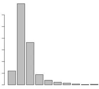
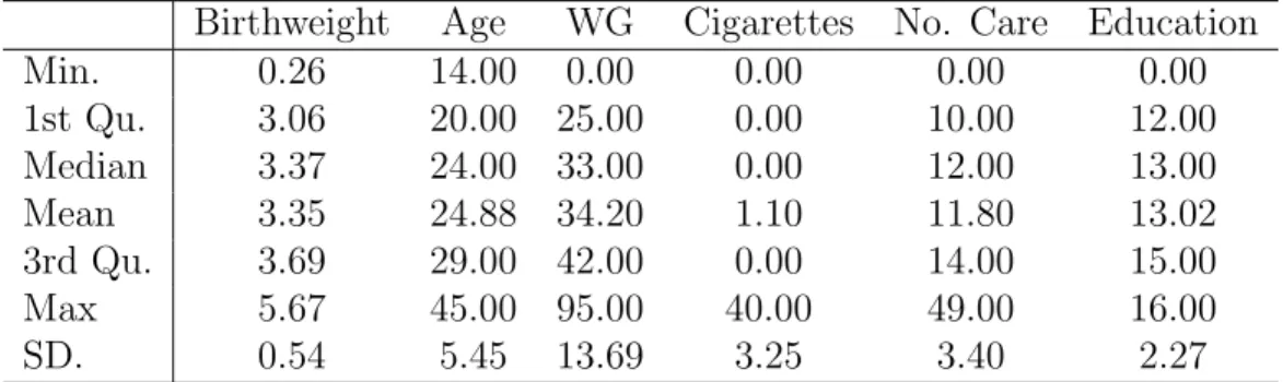
Now we summarize the variables of interest. Out of 13,581 births, there are 6,508 females (proportion 0.4792), and 7,732 mothers are married (proportion 0.5693). Table 1.1 displays statistics for birthweight (measured in kilograms), the mother’s age, the mother’s weight gain during pregnancy (WG), number of cigarettes per day (Cigarettes), number of prenatal care visits (No. Care), and the mother’s years of education for the sample. And Figure 1.1 shows the distribution of the month of first time prenatal care visits.
Our dataset is similar to “1st child” Washington and Arizona datasets of Abre-vaya and Dahl (2008) for the variables that are directly comparable. The number of observations are 45,067 and 56,201 for Washington and Arizona, respectively. For example, the averages of the birthweights of Washington and Arizona data are 3.44 and 3.34 kilograms, respectively, while the average of the birthweights in Wisconsin is 3.35 kilograms. The averages of the ages of Washington and Arizona are 25.27 and 25.23, respectively, while that of Wisconsin is 24.88. The averages of number of prenatal care visits and education in Wisconsin are slightly lower than those of Washington and Arizona. The proportion of male infants are similar for all the births in the three states, but the proportion of married mothers in Wisconsin is much lower than those of Washington and Arizona.
Figure 1.1: Distribution of the Months of First Prenatal Care Visit
1 2 3 4 5 6 7 8 9 10
Month of First Prenatal Care Visit
Frequency
0
1000
3000
5000
Table 1.1: Summary Statistics
Birthweight Age WG Cigarettes No. Care Education
Min. 0.26 14.00 0.00 0.00 0.00 0.00 1st Qu. 3.06 20.00 25.00 0.00 10.00 12.00 Median 3.37 24.00 33.00 0.00 12.00 13.00 Mean 3.35 24.88 34.20 1.10 11.80 13.02 3rd Qu. 3.69 29.00 42.00 0.00 14.00 15.00 Max 5.67 45.00 95.00 40.00 49.00 16.00 SD. 0.54 5.45 13.69 3.25 3.40 2.27
1.5.2
Estimation of Nuisance Parameter
π
0The estimation strategy of nuisance parameters π0(u;t) :=
f0T|X,Y(t|x,y)
f0T|X(t|x) in (1.5) and (1.6) is the same for both the treatment effects of the mother’s age and weight gain during pregnancy. In this section, we describe the details of the estimation procedure using the first treatment effect model, i.e., the mother’s age, as an example.
The mothers’ ages in our sample range from 14 to 45 years old. Therefore, it is natural to treat the mother’s age as a continuous variable in the interval [13,46]. For the estimation of conditional distribution, we assume the relationship logTi−13
46−Ti
=
Xi>θ0 +i, where i is independent of Xi and has density N(0, σ20). The choice of
X is described in the following subsections. The log-ratio form of the dependent variable makes mothers’ age to be limited to [13, 46]. This strategy is similar to the one in the logit model where the probability is confined to [0, 1]. Therefore,
Ti−13
46−Ti =:ηi follows log-normal distribution log-N(X >
i θ0, σ02). The density of T|X is
obtained by calculating the distribution function,
F0T|X(t|x) = P(T ≤t|X =x) = P η ≤ t−13 46−t|X =x =Fη|X t−13 46−t|x = Φ log t−13 46−t−x >θ 0 σ0 ! f0T|X(t|x) =φ logt46−−13t−x>θ0 σ0 ! 1 σ0 1 t−13 + 1 46−t ,
where Φ and φ are distribution and density functions of a standard normal ran-dom variable. For the conditional density of T|X, Y, we assume the relationship log
Ti−13
46−Ti
= Ui>ϑ0+εi, where εi is independent of Ui and has density N(0, ς0).
Therefore, the conditional distribution function
f0T|U(t|u) =φ logt−13 46−t−u >ϑ 0 ς0 ! 1 ς0 1 t−13+ 1 46−t . Hence, we have f0(u, t) = f0T|U(t|u) f0T|X(t|x) = φlog t−13 46−t−u >ϑ 0 ς0 σ0 φlog t−13 46−t−x >θ 0 σ0 ς0 .
1.5.3
Empirical Results
Mothers’ Weight Gain during Pregnancy
The results regarding the mothers’ weight gain during pregnancy show evidence that, after controlling for a mother’s characteristics chosen (i.e., age, marital status, years of education, number of cigarettes per day, and the month of first prenatal care visit), in general, greater weight gain during pregnancy leads to higher birthweight. Figure 1.2 reports the estimates of the average and selected quantiles of the birthweight for different levels of the mother’s weight gain during pregnancy. From the figure, we see that the slopes are relatively larger for low or high weight gain. The shape of the curves resembles a simple cubic function with steeper slopes at the extremes. This implies weight gaining generates higher birthweights at low and high levels of weight gain. For low weight gains, the impact on the birthweight is higher for upper quantiles and relatively mild for low quantiles. However, for the middle range of weight gain, all the curves are relatively parallel. The disaggregated plots with 90% confidence bands are shown in Figure 1.3. The confidence bands in general are relatively wider at the extremes of weight gain due to the sparsity of the data at
Figure 1.2: Mothers’ Weight Gain during Pregnancy and Level of Birthweight 0 20 40 60 80 1 2 3 4 5
Weight Gain During Pregnancy (in pounds)
Bir
thw
eight (in kilogr
ams)
The top and bottom horizontal lines represent the thresholds of high and low birth-weight, respectively. The solid curve is the average of birthweights and the dashed curves are the 90%, 75%, 50%, 25%, and 10% quantiles of birthweights.
the extremes.
Table 1.2 describes treatment effects for selected weight treatment effects. It is divided according to the weight gain interval effects. The first part contains 20 pound effects. The second contains 40 pound effects, and so on until an 80 pound interval. The results show that the impact of gaining weight is positive.
In summary, to produce an infant with healthy birthweight, mothers should gain weight between approximately 20 to 40 pounds. The average birthweight is below 2.5 kilograms for mothers with weight gain less than around 10 pounds and is above 4 kilograms for mothers with weight gain more than around 80 pounds. It seems optimal for pregnant women to gain between 20 to 40 pounds to lower the chances of having LBW or HBW infants.
Figure 1.3: Mothers’ Weight Gain during Pregnancy and Level of Birthweight with 90% Confidence Bands (a) 10% Quantile 0 20 40 60 80 0 1 2 3 4 5
Weight Gain During Pregnancy (in pounds)
Bir
thw
eight (in kilogr
ams) (b) 25% Quantile 0 20 40 60 80 0 1 2 3 4 5
Weight Gain During Pregnancy (in pounds)
Bir
thw
eight (in kilogr
ams) (c) 50% Quantile 0 20 40 60 80 0 1 2 3 4 5
Weight Gain During Pregnancy (in pounds)
Bir
thw
eight (in kilogr
ams) (d) 75% Quantile 0 20 40 60 80 1 2 3 4 5 6
Weight Gain During Pregnancy (in pounds)
Bir
thw
eight (in kilogr
ams) (e) 90% Quantile 0 20 40 60 80 1 2 3 4 5 6
Weight Gain During Pregnancy (in pounds)
Bir
thw
eight (in kilogr
ams) (f) Average 0 20 40 60 80 0 1 2 3 4 5
Weight Gain During Pregnancy (in pounds)
Bir
thw
eight (in kilogr
ams)
The top and bottom horizontal lines represent the thresholds of high and low birth-weight, respectively.
Table 1.2: Treatment Effects of Mothers’ Weight Gain During Pregnancy WG change 10% Qt. 25% Qt. 50% Qt. 75% Qt. 90% Qt. Average 0–20 2.23 2.52 2.68 2.77 2.72 2.53 SD. 0.05 0.07 0.05 0.08 0.07 0.05 20–40 0.37 0.28 0.23 0.25 0.25 0.30 SD. 0.04 0.07 0.06 0.08 0.08 0.06 40–60 0.21 0.20 0.20 0.20 0.23 0.22 SD. 0.05 0.07 0.06 0.09 0.09 0.07 60–80 0.25 0.25 0.28 0.31 0.37 0.30 SD. 0.05 0.08 0.07 0.10 0.11 0.08 0–40 2.59 2.80 2.91 3.03 2.98 2.83 SD. 0.03 0.02 0.02 0.02 0.02 0.02 20–60 0.57 0.48 0.43 0.46 0.48 0.52 SD. 0.04 0.03 0.03 0.03 0.03 0.03 40–80 0.45 0.45 0.48 0.51 0.60 0.51 SD. 0.05 0.05 0.05 0.05 0.07 0.05 0–60 2.80 3.00 3.11 3.23 3.20 3.04 SD. 0.02 0.02 0.01 0.02 0.02 0.01 20–80 0.82 0.74 0.71 0.77 0.85 0.81 SD. 0.03 0.03 0.03 0.04 0.06 0.03 0–80 3.05 3.25 3.39 3.54 3.57 3.34 SD. 0.02 0.02 0.02 0.02 0.05 0.02 Mothers’ Age
The QDRF of the mother’s age on birthweight is downward sloping. For a given age, this negative impact becomes more severe for lower parts of the distribution of birthweights. Although intuitive, this result complements existing results in the literature with three advantages. First, our results can be interpreted as causal effects. Second, we estimate the unconditional quantile and mean of the birthweight for a range of the mothers’ age. Third, unlike using regression framework, our results show that the treatment effects are not confined to be constant or a linear function of ages.
In the current study of the mothers’ age, we control for marital status, years of education, and number of cigarettes per day during pregnancy. It is important to
note that although we are controlling for some characteristics of mothers, we are estimating the unconditional treatment effects. The empirical results for treatment effects of the mother’s age on birthweight reveal that the treatment effect is negative; that is, as expected, the birthweight decreases as the mother’s age increases. Figure 1.4 plots the point estimates for the mean, 10%, 90%, and the three quartiles of birthweights for mothers’ ages from 14 to 45. This impact of the mother’s age on birthweight is negative for all the quantiles. However, for a given age, this impact becomes more severe for lower parts of the distribution of birthweight. In particular, the impact is very prominent for the 10% quantile of mothers after 40 years old. The estimated average birthweight is downward sloping, and more negative at high ages, which is different from the median and is probably capturing the effect of the low quantile. On the other hand, the median birthweight is robust to this feature.
From the disaggregated figures (Figure 1.5) one can see that the 90% confidence bands are narrower in the middle ages because there are more data for that age range. In contrast, we can see that the confidence interval for 10% quantile at the age of 45 is relatively wide.
Table 1.3 describes the treatment effects for selected age treatment effects. The table is divided according to the age interval effects. The first part contains 5 year effects. The second part contains 10 year effects, and so on, until a 30 year interval. Most of them are statistically significant, and negative values show evidence that aging is negatively related to birthweight. Finally, the effect is larger (in absolute values) for the low part of the distribution of birthweights; for example, for a mother aged 25 to 35 years the treatment effect is -0.08 at 10% and -0.05 at 90%.
In general, there are certain risks of having a baby when the mother is too young or too old. Although on average the birthweight is within the “healthy range” between 2.5 and 4 kilograms, our estimates show that mothers younger than 20 years are likely to have HBW infants, while mothers older than 44 years are likely
Figure 1.4: Mothers’ Age and Level of Birthweight 15 20 25 30 35 40 45 2.5 3.0 3.5 4.0 Age Bir thw
eight (in kilogr
ams)
The top and bottom horizontal lines represent the thresholds of high and low birth-weight, respectively. The solid curve is the average of birthweights and the dashed curves are the 90%, 75%, 50%, 25%, and 10% quantiles of birthweights.
Figure 1.5: Mothers’ Age and Level of Birthweight with 90% Confidence Bands (a) 10% Quantile 15 20 25 30 35 40 45 1.8 2.0 2.2 2.4 2.6 2.8 3.0 Mother's Age Bir thw
eight (in kilogr
ams) (b) 25% Quantile 15 20 25 30 35 40 45 2.6 2.8 3.0 3.2 3.4 Mother's Age Bir thw
eight (in kilogr
ams) (c) 50% Quantile 15 20 25 30 35 40 45 3.0 3.2 3.4 3.6 Mother's Age Bir thw
eight (in kilogr
ams) (d) 75% Quantile 15 20 25 30 35 40 45 3.2 3.3 3.4 3.5 3.6 3.7 3.8 3.9 Mother's Age Bir thw
eight (in kilogr
ams) (e) 90% Quantile 15 20 25 30 35 40 45 3.6 3.8 4.0 4.2 4.4 Mother's Age Bir thw
eight (in kilogr
ams) (f) Average 15 20 25 30 35 40 45 3.0 3.2 3.4 3.6 Mother's Age Bir thw
eight (in kilogr
ams)
The thresholds for low and high birthweights are 2.5 kilograms and 4 kilograms, respectively.
to have LBW infants. Therefore, it may be prudent for women who plan to have a baby to do so approximately between 20 and 44 years of age. To prevent female teenagers from having unexpected babies, more education and other forms of help may be needed.
1.6
Conclusion
In this chapter, we first study the identification of a dose-response function with continuous treatment levels. In empirical studies, we usually have observational data. Agents can choose the levels of treatment they desire. Under the ignorabil-ity assumption, we derive moment conditions by which parameters of interest are identified with observational data. Based on the moment conditions, we propose a two-step estimator. Sufficient conditions are provided for the estimator to be consis-tent, converge weakly, and be semiparametric efficient. We study hypothesis testing procedures based on the two-step estimator. More specifically, we are interested in testing the null hypothesis that a DRF β(t) = r(t) with t ∈ T for known or unknown r(t). Because the parameters are infinite dimensional and the weak limits of test statistics are not standard, we use the bootstrap method when conducting inferences. Finally, we apply our estimation methods to the study of unconditional effects of mothers’ weight gain during pregnancy and age on infants’ birthweight, illustrating the usefulness of the new estimator.