STABILITY OF HIGH-SPEED, THREE-DIMENSIONAL BOUNDARY LAYERS
A Dissertation by
STUART ALEXANDER CRAIG
Submitted to the Office of Graduate and Professional Studies of Texas A&M University
in partial fulfillment of the requirements for the degree of DOCTOR OF PHILOSOPHY
Chair of Committee, William S. Saric Committee Members, Helen L. Reed
Rodney D. W. Bowersox Simon W. North
Eli Reshotko
Head of Department, Rodney D. W. Bowersox
May 2015
Major Subject: Aerospace Engineering
ABSTRACT
Boundary-layer experiments are performed in the low-disturbance, Mach 6 Quiet Tunnel (M6QT) at Texas A&M University. The experiments are focused specifically on investigating the physics of two three-dimensional phenomena in hypersonic boundary-layer stability and transition: the breakdown of second-mode waves and the growth and breakdown of crossflow waves. In order to enable these experiments, a new, three-dimensional probe traversing mechanism was designed and constructed. In order to investigate the breakdown of second-mode waves, experiments are conducted on a flared cone with a 5◦ half angle at the tip at zero angle of attack. Experiments were typically performed at unit Reynolds number Re0 ≈10×106/m
with a slightly hot wall, T /Taw ≈1.05. A new, durable method of roughness element
application is discussed for the purpose of exciting the unstable waves. Hot-wire measurements were made of the boundary layer and it is shown that even with roughness elements, transition to turbulence does not occur on the model. Therefore, the expected Λ vortices are not observed.
The crossflow instability in a hypersonic boundary layer is studied on a7◦ right circular cone at 5.6◦ angle of incidence. Experiments were performed at Re0 ≈ 10×106/m with an adiabatic wall. Hot wire measurements are made at a series
of axial locations to generate contours of streamwise mass flux. The stationary vortex structure is shown through its saturation. Traveling waves are observed in the expected frequency range, 10 kHz to 60 kHz, predicted by computations and are located generally in the high-speed troughs in the vortex structure. Secondary instability is observed between 80 kHz and 130 kHz. Frequency scaling and location is shown to agree with low-speed experiments and good preliminary agreement with
hypersonic computations is obtained. Transition does not naturally occur on the model. Distributed roughness is applied to the tip in order to excite crossflow and cause transition. Transition is shown to occur with the rough tip, but is not likely a result of crossflow.
ACKNOWLEDGEMENTS
This work would not be possible without the input and support provided by a number of people. First and foremost, I offer my thanks to my committee chair and advisor, Dr. William Saric. The opportunities for growth I have been afforded under his guidance have been invaluable. I am truly grateful for the chance to learn from his extensive experience and the opportunity I have had to truly take ownership of the research under his guidance.
I would also like to thank Dr. Rodney Bowersox for all of the discussions and advice throughout this process. Dr. Helen Reed has also been especially helpful, both for her computational support and the discussions that often helped me look at the problems from a different perspective. The rest of my committee, Dr. Simon North and Dr. Eli Reshotko, are also acknowledged for their ongoing support.
These experiments involved many long days and nights, and I am indebted to my colleagues at the National Aerothermochemistry Laboratory for their help and cooperation. In particular I would like to thank Dr. Jerrod Hofferth and Dr. Ray Humble for all the discussion and advice they’ve provided.
Finally, I’d like to thank Ms. Colleen Leatherman for all of the support and general cheerfulness over the last several years. The lab would not function properly without her.
This work was principally funded by NASA and AFOSR through the National Center for Hypersonic Laminar-Turbulent Transition Research (AFOSR Grant FA9550-09-1-0341) and through the Texas A&M Foundation through the George Eppright ‘26 Chair in Engineering.
NOMENCLATURE
Acronyms DNS direct numerical simulation DRE discrete roughness element FSD focusing schlieren deflectometry
IR infrared
LaRC Langley Research Center LFC laminar flow control LST linear stability theory
LPSE linear parabolized stability equations
M6NTC Advanced Mach 6 Quiet Tunnel in the Nozzle Test Chamber M6QT Mach 6 Quiet Tunnel
NAL National Aerothermochemistry Laboratory NASA National Aeronautics and Space Administration NPSE nonlinear parabolized stability equations
NS Navier-Stokes
QTC quiet test core
TAMU Texas A&M University TAMU 7DC TAMU 7-degree cone model TPS thermal protection system
Symbols
d hot-wire diameter
D d/dy
kc circumferential wavenumber [1/2π]
` hot-wire active length
M Mach number
M relative Mach number
Me edge Mach number
N N-factor, ln(A/A0)
r radial coordinate
Re Reynolds number, ρuL/µ
Red Reynolds number based on wire diameter
Rekk Reynolds number at roughness height, k, using flow conditions at k
Retr Reynolds number at the transition location Re0 unit Reynolds number
T temperature
Taw adiabatic wall temperature
V voltage
z axial coordinate
Greek symbols
α α =αr+iαi, wavenumber in the streamwise direction
β β =βr+iβi, wavenumber in the spanwise direction
λ wavelength
θ azimuthal coordinate
φc cone half angle
ω angular frequency
Subscripts
aw adiabatic wall condition fs free-stream condition
t total conditions
tr transition conditions w near-wall condition
TABLE OF CONTENTS Page ABSTRACT . . . ii DEDICATION . . . iv ACKNOWLEDGEMENTS . . . v NOMENCLATURE . . . vi TABLE OF CONTENTS . . . ix
LIST OF FIGURES . . . xii
LIST OF TABLES . . . xv
1. INTRODUCTION . . . 1
1.1 Background and motivation . . . 1
1.2 Introduction to the transition process . . . 2
1.3 Linear stability theory . . . 5
1.4 The Mack mode . . . 9
1.4.1 Instability mechanism and background . . . 9
1.4.2 Motivating studies . . . 11
1.5 The crossflow instability . . . 12
1.5.1 Instability mechanism . . . 12
1.5.2 Crossflow in compressible boundary layers . . . 16
1.6 Experimental objectives . . . 17
1.6.1 Three-dimensional probe traverse . . . 17
1.6.2 The second mode . . . 17
1.6.3 High-speed crossflow . . . 18
2. EXPERIMENTAL SETUP & TECHNIQUES . . . 19
2.1 The Mach 6 Quiet Tunnel Facility . . . 19
2.1.1 Tunnel history . . . 19
2.1.2 Re-establishment and flow quality . . . 20
2.1.3 Tunnel design . . . 20
2.1.4 Infrastructure . . . 24
2.2.1 Flared cone . . . 26 2.2.2 Straight cone . . . 28 2.2.3 Roughness configurations . . . 29 2.3 Traversing system . . . 31 2.3.1 Design considerations . . . 31 2.3.2 Design details . . . 33
2.4 Instrumentation and data acquisition system . . . 40
2.5 Measurement techniques . . . 41
2.5.1 Constant-temperature anemometry . . . 42
2.5.2 Infrared thermography . . . 49
2.5.3 Focusing schlieren deflectometry . . . 49
2.6 Operating procedure . . . 51
3. RESULTS: THE MACK MODE ON A FLARED CONE . . . 53
3.1 Overview . . . 53
3.2 Model alignment . . . 55
3.3 Operating conditions . . . 55
3.4 Two-dimensional strip and DRE . . . 57
3.4.1 Roughness elements . . . 57
3.4.2 Hot-wire measurements . . . 58
3.5 Ovoid decal DRE . . . 60
3.5.1 Roughness elements . . . 60
3.5.2 Hot-wire measurements . . . 62
3.6 Discussion . . . 63
4. RESULTS: CROSSFLOW INSTABILITY ON A YAWED CONE . . . 67
4.1 Overview . . . 67
4.2 Operating conditions . . . 67
4.3 Infrared flow visualization and transition detection . . . 68
4.4 Hot-wire measurements . . . 70 4.4.1 z = 350 mm . . . 70 4.4.2 z = 360 mm . . . 74 4.4.3 z = 370 mm . . . 74 4.4.4 z = 380 mm . . . 78 4.4.5 z = 390 mm . . . 78
4.5 Traveling crossflow and first-mode waves . . . 82
4.6 Secondary instability . . . 85
4.7 Mode growth and interaction . . . 87
4.7.1 Mode growth and saturation . . . 87
4.7.2 Nonlinear interactions . . . 89
5. RESULTS: DISTRIBUTED ROUGHNESS ON A YAWED CONE . . . 93
5.1 Overview . . . 93
5.3 Infrared flow visualization . . . 94
5.4 Hot-wire measurements . . . 97
6. CONCLUSIONS AND FUTURE WORK . . . 101
6.1 Conclusions . . . 101
6.1.1 Mack-mode breakdown . . . 101
6.1.2 Natural crossflow . . . 102
6.1.3 Breakdown of crossflow vortices . . . 103
6.2 Future considerations and recommendations . . . 104
6.2.1 Mack-mode breakdown . . . 104
6.2.2 Future crossflow experiments . . . 105
6.2.3 General recommendations . . . 106
REFERENCES . . . 110
LIST OF FIGURES
FIGURE Page
1.1 The transition road map . . . 3
1.2 The Mack mode in a typical hypersonic, conical boundary layer. . . . 9
1.3 Diagram of a typical crossflow boundary-layer profile. . . 13
1.4 Streamwise velocity at constant-chord measured with a hot wire on a subsonic swept wing from Saricet al. (2003) (originally Reibert et al., 1996). . . 14
2.1 Cutaway of M6QT components. . . 21
2.2 M6QT nozzle annotated with the quiet test core (QTC) and associated features. . . 21
2.3 M6QT settling chamber and contraction, annotated with internal features. . . 22
2.4 M6QT nozzle dimensions and detail. Inset is a close-up of the throat and bleed gap. . . 23
2.5 Diagram of the LaRC 93-10 flared cone. . . 26
2.6 Diagram of the TAMU 7DC right-circular cone. . . 27
2.7 A typical power spectrum across the composite distributed roughness. 30 2.8 Three-dimensional traversing mechanism affixed to 7◦ cone model. . . 32
2.9 Cylindrical traverse system with the carriage removed (front view). . 34
2.10 Cylindrical traverse system with the carriage removed (side view). . . 35
2.11 Close-up view of the carriage and ring assembly and gear orientation. 36 2.12 Isometric view of the carriage housing the motion stages. . . 37
2.13 Traverse carriage and radial arm (front view). . . 38
2.14 Traverse carriage and radial arm (side view). . . 39
2.16 Detailed schematic of the focusing schlieren system. . . 50
3.1 Typical spectrogram produced during a pressure sweep used for cone alignment. . . 56
3.2 Model surface temperature on the LaRC 93-10 flared cone over the course of one tunnel run. . . 57
3.3 Flow contours at z = 493 mm over the 93-10 flared cone with the 2-D strip and DREs. . . 59
3.4 A series of azimuthal boundary layer scans atr = 1.575 mm over the 93-10 flared cone with two layers of tape and DREs. . . 60
3.5 Diagram showing the layout of ovoid decal DREs. . . 62
3.6 Flow contours atz = 493 mm over the 93-10 flared cone with ovoid DRE decals. . . 64
3.7 Azimuthal boundary layer scans atr = 1.65 mm over the 93-10 flared cone with 3 layers of decal DREs. . . 65
4.1 Model surface temperature on the TAMU 7DC over the course of one tunnel run. . . 68
4.2 IR thermography depicting crossflow vortices on TAMU 7DC. . . 69
4.3 Hot-wire data atz = 350 mm. . . 71 4.4 Band-passed data at z = 350 mm . . . 73 4.5 Hot-wire data atz = 360 mm. . . 75 4.6 Band-passed data at z = 360 mm . . . 76 4.7 Hot-wire data atz = 370 mm. . . 77 4.8 Band-passed data at z = 370 mm . . . 79 4.9 Hot-wire data atz = 380 mm. . . 80 4.10 Band-passed data at z = 380 mm . . . 81 4.11 Hot-wire data atz = 390 mm. . . 83 4.12 Band-passed data at z = 390 mm . . . 84
4.14 Amplitude growth of unstead and stationary modes. . . 88
4.15 Crossflow growth plot from White & Saric (2005) . . . 89
4.16 Bicoherence plots at (a)z = 370 mm and (b)z = 380 mm . . . 91
5.1 Initial IR thermography on the TAMU 7DC with rough tip. . . 95
5.2 IR thermography on the TAMU 7DC with rough tip. . . 96
5.3 Azimuthal boundary layer scans with the rough tip. . . 98
LIST OF TABLES
TABLE Page
2.1 Motion specification and details for the azimuthal traversing system . 36 2.2 M6QT operating envelope. . . 51
1. INTRODUCTION
1.1 Background and motivation
Boundary-layer trasition on hypersonic vehicles is of paramount importance to their safe and efficient design as a result of the substantial increase in thermal load associated with a turbulent boundary layer. Substantial progress has been achieved in recent years as a result of cooperation between experiments, computations, and theory, particularly for the class of flows dominated by Mack’s (1984) acoustic second-mode instability (Fedorov, 2011). Comparatively little attention has been paid to the crossflow instability, which dominates the three-dimensional boundary layers that arise on common hypersonic vehicle geometries such as swept surfaces and conical bodies at angle of attack.
Hypersonic vehicle designs are extraordinarily sensitive to the state of the boundary layer. These vehicles owe their survival to their ability to manage the thermal load due to aerodynamic heating and their ability to generate thrust to efficient mixing of the fuel and air. As turbulence enhances both heating and mixing, developing a physics-based theory for boundary-layer transition in hypersonic flows is a key enabling technology for the development of hypersonic vehicles. Despite its importance, such a predictive tool does not yet exist and vehicle designers have been forced to rely on empirical and vehicle-specific correlation methods with limited utility such as Reθ/Me
(Reshotko, 2007). Poor predictive tools have led to the over-design of the thermal protection system on most hypersonic vehicles to date and scramjet engines continue to be plagued by poor performance and unstart related to insufficient understanding of the transition process (Borg & Schneider, 2008).
in the study of the crossflow instability at subsonic speeds and the experimental data on swept-wing models are quite rich (Saric et al., 2003; White & Saric, 2005). However, a number of practical issues have led to the scarcity of similar experiments in hypersonic flows. The cost of flight-testing hypersonic vehicles is often prohibitive, as is the development of new hypersonic, low-disturbance wind tunnels, which are required for conducting meaningful transition experiments (Schneider, 2007). At present, only two such facilities are operational: a Ludwieg tube at Purdue University and a blowdown wind tunnel at Texas A&M University.
The present study seeks to fill this gap in experimental hypersonic boundary-layer data. The Mach 6 Quiet Tunnel (M6QT) facility at Texas A&M University, featuring a thirty-second run time and three-dimensional traversing mechanism, is uniquely suited for boundary layer measurements of this kind. Of particular interest is the degree to which the primary and secondary instability mechanisms mimic their subsonic counterparts and how well existing hypersonic theory and computations match with these experimental data.
1.2 Introduction to the transition process
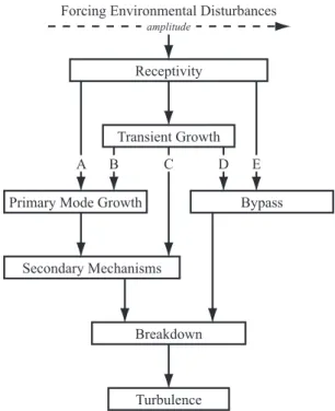
The study of boundary-layer transition has been of theoretical and practical interest to the fluid dynamics community since the turn of the century, when Reynolds (1883) made his famous observations of turbulence in pipe flows and Prandtl (1904) developed the theory of the boundary layer. The studies over the ensuing century have shed light on a large portion of the process and are often distilled into a graphical overview known as the transition road map (Figure 1.1), which lays out the various paths a boundary layer may take from its laminar inception to the onset of turbulence. A boundary layer is a highly nonlinear dynamical system subject to a variety of stable and unstable waves, some of which may grow to such amplitude as to break down to
Receptivity
Transient Growth
Primary Mode Growth
Secondary Mechanisms
Breakdown
Bypass
Turbulence
Forcing Environmental Disturbances
A B C D E
amplitude
Figure 1.1: The transition road map
turbulence.
The genesis of the small boundary-layer disturbances lies in the free stream, where small fluctuations in the external flow (e.g. sound, vorticity, or entropy) interact with features of the surface such as roughness and become entrained in the incipient boundary layer through a process known as receptivity (Saric et al., 2002). The receptivity process itself is poorly understood, but the end result is a spectrum of small disturbances within the boundary layer, some of which are dynamically unstable. The stability and transition problem therefore amounts to a nonlinear initial value problem governed by the Navier-Stokes equations whose initial conditions are those provided by the receptivity process. The path in Figure 1.1 followed for a given boundary layer depends on the magnitude of the initial conditions.
disturbances and receptivity. The road map lays out the various paths to turbulence such that the phenomena are ordered from left to right by increasing initial disturbance amplitude. The most commonly observed path in flight, and that which is of greatest interest to the present work, is path A. This path begins with the smallest initial disturbances and comprises four stages: receptivity, primary-mode growth, secondary mechanisms, and breakdown to turbulence. The initial growth phases of both the primary wave and the secondary mechanisms may often be modeled linearly. Continued mode growth eventually reaches the point where nonlinear terms can no longer be neglected and play a major role in the remainder of the transition process.
For very large initial disturbances (path E), the boundary layer undergoes a process known as bypass. In these situations, the boundary layer effectively bypasses all known boundary-layer instability mechanisms and transitions directly to turbulence. This path represents all instances of boundary layers for which no mechanism has yet been found to explain the observed transition.
For initial disturbances that fall between the levels required forpaths A and E, a boundary layer may undergo transient growth. Transient growth results when two nonorthogonal modes, which are each linearly stable, interact to produce a resultant mode that grows algebraically (Landahl, 1980; Gustavsson, 1991; Butler & Farrell, 1992; Schmid et al., 1993; Trefethen et al., 1993; Reshotko, 2001) even while both individual modes decay. This slowly-growing disturbance can then lead to one of three phenomena depending on the intitial disturbance amplitude. Relatively small amplitudes may follow path B, whereby the disturbance energy from the transient growth helps amplify primary instability mechanisms in the boundary layer. For larger initial amplitude, transient growth may result in modification to the mean flow that is large enough to lead directly to the development of secondary instability mechanisms, cutting out primary modes altogether (path C). Finally, for large initial
amplitude, the process may follow path D and the modified boundary layer may be so unstable that it triggers bypass transition.
1.3 Linear stability theory
Much of the current theoretical understanding of the laminar-turbulent transition process is grounded in linear stability theory (LST). A boundary layer is a nonlinear dynamical system subject to instability in the same way as any other dynamical system. The highly nonlinear nature of the full Navier-Stokes (NS) equations makes direct solution difficult; however, the initial growth of small-amplitude disturbances within the boundary layer can be accurately described through a much simpler linear stability analysis. LST is treated at length by Mack (1984). However, several important features of the compressible stability problem can be highlighted by a brief discussion of the inviscid problem.
A LST analysis begins by assuming small perturbations to the full NS equations. These are implemented by writing the flow quantities as a sum of a time-independent mean component and a small fluctuating component, for example
u(~x, t) =U(~x) +u0(~x, t), (1.1) where~xis the spatial coordinate and t is time. These are then substituted into the dimensionless, compressible NS equations, continuity equation, and energy equation. The mean flow terms identically satisfy the NS equations and fall out of the equations. Assuming the perturbations remain small, the equations are linearized. This leaves a six-equation system describing the evolution of the perturbation quantities. At this point, the analysis may follow a number of different routes. Typically, the flow is
assumed to be locally parallel and a normal mode solution is assumed of the form
q(x, y, z, t) = ˆq(y) exp [i(αx+βz−ωt)], (1.2) whereq is simply a variable representing any of the disturbance quantities. α and β represent the x and z components of the wavenumber vector,~k, and ω is the angular frequency of the disturbance. In general, alphaandβ are complex and ω is real. The result is an eighth-order system of six equations describing the linear stability of the small perturbations.
The equations can be further manipulated by introducing the relative Mach number
M = (αU +βW −ω) (α2+β2)1/2
Me
T1/2. (1.3)
The physical meaning of this “relative Mach number” is revealed by rewriting the definition as follows: M = ~ V ·~k k − ω k Me T1/2 =M||− c a. (1.4)
The relative Mach number therefore represents the Mach number of the mean flow in the direction of ~k, (Mk), relative to the phase speed (c). Using this definition, the inviscid stability equations can be written in the form
∂2ψ ∂y2 + 1−M2∂ 2ψ ∂x2 +f M , ψ, ∂ψ ∂y ! = 0. (1.5)
The analytical character of Eq. 1.5 changes depending on the value of M2. When M2 <1, the solutions are elliptic and a unique α exists for a given c (Lees & Lin, 1946). All subsonic boundary layers fit into this category. However, when M2 >1,
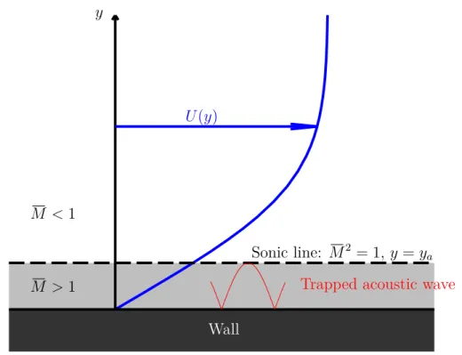
the solutions are hyperbolic and an infinite series of wavenumbers may satisfy the governing equation. This leaves open the possibility that many inviscid modes may exist in a given supersonic boundary layer. These modes only exist in the region whereM >1 (between some sonic line, ya, and the wall) and represent a family of
trapped acoustic waves reflecting back and forth between the wall and the sonic line. Depending on the flow conditions, these additional acoustic modes may be the most unstable (Mack, 1969, 1984).
It is also important to note that Rayleigh’s criterion for inviscid instability in an incompressible flow does not hold for compressible flows. Instead, a modified form, the generalized inflection point, exists. For a compressible boundary layer, the necessary and sufficient condition for inviscid instability is that at some point ys > yc,
D(ρDU) = 0. (1.6)
Here, yc is the point in the boundary layer where U(yc) = 1−1/Me,Me is the edge
Mach number, D= d/dy, and y represents the wall-normal direction. As a result, in contrast to the incompressible case, even a compressible boundary layer over a zero-pressure-gradient flat plate is always unstable to inviscid waves (Mack, 1984; Reed et al., 1996).
Historically, the so-calledeN method proposed independently by Smith &
Gam-beroni (1956) and Van Ingen (1956) has been used to correlate LST predictions with transition in experiments and flight. In this method, the transition Reynolds number, Retr, is correlated with the amplification factor, N, defined as
N = ln A
A0
Here,Ais the disturbance amplitude at a given location andA0 is the initial amplitude.
Typically, the value ofN at Retr for a given geometry is determined empirically and used to predict transition in other situations. Since eN is simply an amplitude
ratio, aN does not retain any information about receptivity, its effect on the transition process, or the underlying instability mechanisms that lead to transition. As a result, the eN method must be used with care and only when the underlying physics and transition mechanisms of a given flow are understood (Arnal, 1994; Reedet al., 1996).
Two-dimensional disturbances such as Tollmien-Schlichting (T-S) waves or the Mack mode (see section 1.4) are insensitive to small surface roughness and typically remain linear for much of their growth history. TheeN method is therefore well-suited
to these problems and performs very well provided that the dominant instability mechanisms and the free-stream disturbance levels are the same in each application (Arnal, 1994).
In three-dimensional flows,eN is a poor predictor of Retr for a number of reasons.
Three-dimensional waves such as stationary crossflow and Görtler vortices are extraor-dinarily sensitive to surface roughness, complicating comparisons between different experiments and flight. Further, these disturbance are characterized by the rapid development of nonlinear mean flow modification and saturation behavior that is not captured by linear theory. The result is that there is considerable scatter in the predicted and measured values of N for a given flow measured on different models or in different tunnels (Reed et al., 1996).
However, owing to the ubiquity of this method and its historical significance, the N factor is frequently used in other contexts within the body of stability research, including in three-dimensional flows. As many boundary-layer instabilities exhibit exponential growth, N is a convenient method for reporting mode amplification relative to some computed or measured initial state.
Wall
Trapped acoustic wave
Sonic line: M2 = 1, y=ya
M >1 M <1
U(y)
y
Figure 1.2: The Mack mode in a typical hypersonic, conical boundary layer.
1.4 The Mack mode
1.4.1 Instability mechanism and background
The multimodal nature of inviscid waves in hypersonic boundary layers is in stark contrast to flows of lower speed. In subsonic and low-supersonic applications, only the first mode is unstable; the others are stable and effectively decoupled from the first mode (Fedorov, 2011). The first mode includes instabilities such as the familiar T-S waves, which dominate the transition process in subsonic flows not subject to three-dimensional instabilities such as crossflow.
In hypersonic flows, the acoustic modes exist simultaneously with the first mode and represent acoustic waves in the M2 > 1 region of the boundary layer. This critical layer acts as an acoustic waveguide, trapping these waves between the sonic
line and the wall (Figure 1.2). The first of these acoustic modes is typically termed the “second-mode instability” or the “Mack mode”. The “second mode” nomenclature derives from the fact that it is the second mode of inviscid instability in the boundary layer and is not a reflection of the multimodal nature of the acoustic instability. As such, the latter of the two terms, the “Mack mode,” will be used henceforth to avoid confusion.
In contrast to subsonic T-S waves, which are two-dimensional and streamwise in nature, their supersonic counterparts, first-mode waves, become increasingly oblique with increasing Mach number. Up to Me≈2.2, the first mode is the only instability
present in a flat plate or cone boundary layer, at which point the Mack mode exhibits appreciable growth. At Me≈4, the Mack mode becomes the dominant instability
mechanism in the boundary layer (Mack, 1969, 1984).
Mack mode waves are two dimensional and tuned with the boundary layer thickness. The wavelength very nearly follows the relationship λ≈2δ. The small wavelength combined with the large phase velocity means that these waves typically exhibit very high frequencies ranging from O(105) Hz to O(106) Hz in most situations, which
complicates their measurement.
The Mack mode is highly sensitive to wall temperature and pressure gradient (Mack, 1984). Mack-mode waves are destabilized by an adverse pressure gradient, motivating the use of flared cone models in much of the experimental studies. The Mack mode is also destabilized substantially by wall cooling (this is opposite the behavior of the first mode). As a result, cooled models have been developed and represent a promising avenue of research.
1.4.2 Motivating studies
The Mack mode has been the subject of considerable study, both experimental and numerical. A detailed summary of Mack-mode research is given in Fedorov (2011). However, several studies in particular should be noted as motivation for the present work.
Much of the early experimental studies of Mack-mode waves can be found in experiments performed such as those by Demetriades (1974), Kendall (1975), Stetson
et al. (1983), and Stetson & Kimmel (1992). Altogether, studies such as these made substantial progress toward our present understanding of hypersonic boundary-layer stability and the accuracy of LST toward these flows. However, in each case (and many others), these experiments have been performed in conventional hypersonic wind tunnels where free-stream disturbances are at least an order of magnitude larger than those encountered in a flight environment. While they did match up well with LST, recall from Figure 1.1 that increased free-stream disturbance levels can lead to dramatically different downstream behavior. In order to properly study the behavior of hypersonic boundary layers relevant to flight vehicles, it is therefore necessary to perform experiments in specialized low-disturbance facilities (Schneider, 2007).
Highlighting the recent computational work are a pair of studies by Sivasubrama-nian & Fasel (2012a,b). In these studies, a broadband wavepacket was first simulated using direct numerical simulation (DNS) showing evidence of nonlinear interaction of various streamwise and oblique modes. Following up on this, the most unstable two-dimensional wave was artificially stimulated along with the oblique wave found to be most likely to interact with the primary wave. The growth of this disturbance led ultimately to a K-type breakdown featuring Λ vortices reminiscent of the breakdown of T-S waves on an incompressible flat plate reported by Klebanoff et al. (1962).
Such a phenomenon, if confirmed experimentally, represents a fundamental similarity between the breakdown of high- and low-speed flows despite the substantial differences in the conditions under which these instability modes dominate.
1.5 The crossflow instability
1.5.1 Instability mechanism
The second mode is commonly the most unstable on unswept surfaces and conical geometries at zero angle of incidence. However, on other geometries common in high-speed flight (for example swept surfaces, cones at nonzero angle of incidence, or rotating axisymmetric bodies) the crossflow instability becomes occurs at lower Re and is the dominant instability mechanism in the transition process.
The crossflow instability arises in regions with a pressure gradient and curved streamlines. Using the example of a swept wing, the inviscid streamlines are curved as a result of the combined influence of sweep and the pressure gradient. The pressure gradient, being nonparallel to the streamlines, has a component normal to the inviscid streamlines which corresponds to the centripetal force for the curved streamlines. While the pressure gradient is constant throughout the boundary layer, the velocity is reduced near the wall. The pressure gradient therefore creates a nonzero stream-normal velocity component known as the crossflow component.
Figure 1.3 depicts a typical three-dimensional boundary layer subject to the crossflow instability. The crossflow boundary layer is precisely zero at the wall (no-slip) and smoothly approaches zero aszapproaches infinity. It therefore necessarily features an inflection point. While the streamwise boundary layer is often inviscidly stable in low-speed flows, the inflection point in the crossflow boundary layer signals inviscid instability in the 3-D boundary layer. In high-speed flows, it provides a generalized inflectional instability in addition to that which already exists in the streamwise
xt
yt
zt
ut
wt
streamwise component crossflow component
inflection point
Figure 1.3: Diagram of a typical crossflow boundary-layer profile.
profile. The wavenumber vector ~k of the resulting crossflow waves points in the crossflow direction (zt in Figure 1.3).
The crossflow instability in subsonic and low-supersonic flows has been the subject of considerable research since the foundational studies of Gray (1952) and Gregory
et al. (1955). Early work focused on the boundary layer over a rotating disc, which was exactly solvable and served as a convenient canonical case for researchers at the time. A comprehensive review of the early literature can be found in Reed & Saric (1989) and of subsequent studies in Saricet al. (2003).
Both experiments and theory exhibit the existence and amplification of both stationary and traveling crossflow waves. Despite the existence of both modes, transition is usually dominated by one or the other rather than a combination of the two. While traveling modes are generally more unstable than are the stationary modes according to linear theory, stationary modes are often those observed causing transition
Figure 1.4: Streamwise velocity at constant-chord measured with a hot wire on a subsonic swept wing from Saric et al. (2003) (originally Reibert et al., 1996).
in flight-like environments at subsonic and low-supersonic speeds. The reason for this lies in the receptivity process. The initial amplitudes for traveling waves are highly dependent on the free-stream turbulence levels, and the primary determining factor in whether traveling or stationary waves dominate is the level of turbulence in the test environment. Traveling waves tend to dominate in high-turbulence environments such as “noisy” wind tunnels, while stationary waves dominate in low-turbulence environments such as in flight or in low-disturbance wind tunnels (Deyhle & Bippes, 1996; Bippes, 1999).
The stationary waves manifest as approximately streamwise, corotating vortices. Since stationary crossflow modes grow relatively slowly, LST is sufficient to predict
the initial details of the instability (i.e. unstable wavenumbers). However, stationary crossflow vortices are body-fixed and nearly aligned with the inviscid streamlines; therefore, the integrated effect of the otherwise weak disturbances in v and w draw regions of the flow with O(1) momentum low into the boundary layer while injecting low-momentum fluid into the upper portion boundary layer, depicted on a subsonic swept wing in Figure 1.4 from (Saric et al., 2003). The figure shows a contour of streamwise velocity measured using a hot-wire probe and features the characteristic altered basic state of a crossflow-dominated boundary layer, which leads rapidly to nonlinearity and quickly invalidates linear theory (Dagenhart et al., 1989a,b; Bippes & Nitschke-Kowsky, 1990; Bippes et al., 1991; Deyhle et al., 1993; Reibert et al., 1996). For the determination of more useful statistics such as integrated mode growth, nonlinear techniques must therefore be used such as the parabolized stability equations (Herbert, 1997; Haynes & Reed, 2000).
As the nonlinear wave grows, the mean-flow distortion produced by the vortices becomes more pronounced, resulting in alternating high- and low-momentum regions in the boundary layer. As these low-momentum upwellings grow more pronounced, they begin to roll over in the upper region of the boundary layer, resulting in highly unstable boundary layers with multiple inflection points. These late-developing inflection points lead to secondary inviscid instability (Kohama et al., 1991; Malik
et al., 1994; Wassermann & Kloker, 2002; White & Saric, 2005; Bonfigli & Kloker, 2007). It is these secondary instabilities rather than the primary wave that eventually cause the breakdown to transition.
It was predicted by Maliket al. (1996) and confirmed experimentally by White & Saric (2005) that two classes of secondary instability exist in the crossflow boundary layer. Type-I modes are dominated by the ∂U/∂z extrema, and type-II modes are dominated by the∂U/∂yextrema. In most situations, the type-I secondary instability
modes have been observed first, followed rapidly by type-II modes.
1.5.2 Crossflow in compressible boundary layers
The overwhelming majority of crossflow research has been performed at subsonic and low-supersonic velocities. The underlying mechanism leading to crossflow, pres-sure gradient and curved streamlines, is the same across all Mach numbers. As such, crossflow waves in hypersonic flows are expected to behave qualitatively similar to their lower-speed counterparts. However, experiments in hypersonic flows dominated by crossflow instability are few and include no detailed boundary-layer experiments.
Early experiments such as those by Stetson (1982) focused on the movement of the transition front as a function of angle of attack and nose bluntness rather than the nature of the instability waves. More recently, a number of experiments have been performed in impulse facilities where run times restrict measurement techniques to surface measurements of pressure, temperature, and heat transfer (see, for example, van den Kroonenberg et al., 2010; Swanson & Schneider, 2010; Muñoz et al., 2014; Ward, 2014).
Experiments by Schueleet al. (2013) were performed in a Mach 3.5 blowdown facility on a yawed cone boundary layer using point measurements. However, the goal of this study was to test the extension of the use discrete roughness elements (DREs) for flow control, first pioneered by Saric et al. (1998), to a high-speed boundary layer. Further, The Pitot measurements performed were of limited bandwidth and were unable to resolve the secondary instability.
While experiments have not yet explored the structure and breakdown of hyper-sonic crossflow waves, several computational studies have been performed on this topic on cones at angle of attack. Balakumar & Owens (2010) performed a DNS on a cone with both a smooth tip and two patterns of DREs. Kuehl et al. (2012)
and Perez et al. (2013) have performed PSE calculations, both linear (LPSE) and nonlinear (NPSE) using a new code on the same geometry as Balakumar & Owens (2010) with the smooth tip. These PSE computations have shown good agreement with the DNS. Gronvall et al. (2012) performed a DNS on the same geometry with distributed roughness placed at the tip.
The surface methods popular in the above experiments have compared well with the above computations. However, no suitable experiment yet exists for comparison with the more detailed aspects of the boundary layer predicted by computations. Further, the hallmark features of low-speed crossflow such as stationary mode saturation, the development of secondary instability, and the ultimate breakdown mechanism(s) have yet to be confirmed experimentally in hypersonic flows.
1.6 Experimental objectives
1.6.1 Three-dimensional probe traverse
The planned experiments in M6QT are to be three-dimensional. As such, the first objective and key enabling technology for these studies is the development of a new probe traversing mechanism. This mechanism should work on axisymmetric models with either straight-walled or flared geometry.
1.6.2 The second mode
Previous experiments by Hofferth (2013) have documented the early growth and onset of nonlinear behavior in the second-mode-dominated boundary layer over a flared cone. Further, computations by Sivasubramanian & Fasel (2012a,b) and Reed (private communication) have indicated that the ultimate breakdown mechanism may be fundamentally similar to that of Tollmien-Schlichting waves on the low-speed flat plate. One objective of this study is therefore to promote the breakdown of second-mode waves and explore the characteristics of this breakdown.
1.6.3 High-speed crossflow
The crossflow instability is expected to be dominant on a wide class of common geometries on hypersonic vehicles. Despite this, it has been studied only lightly under such conditions and no detailed boundary-layer measurements exist. The resulting uncertainty surrounding the crossflow instability in the hypersonic regime partially motivated the nearly 2-D design of the X-43A. The final objective of this study is therefore to perform the first such boundary-layer experiments on hypersonic crossflow with the goal of providing data at the level of detail applied to low-speed flows. Questions of particular interest include:
• Do stationary waves still dominate in low-noise environments? • Do stationary and traveling waves coexist?
• Do stationary waves exhibit saturation, and if so, at what amplitude?
• At what point does secondary instability occur and which type develops first? Do they lead rapidly to breakdown?
2. EXPERIMENTAL SETUP & TECHNIQUES
2.1 The Mach 6 Quiet Tunnel Facility
2.1.1 Tunnel history
The Mach 6 Quiet Tunnel (M6QT) is a hypersonic, low-disturbance wind tunnel facility at Texas A&M University (TAMU) that traces its roots to the Advanced Mach 6 Pilot Quiet Tunnel in the Nozzle Test Chamber (M6NTC) developed at the NASA Langley Research Center (LaRC). The culmination of a 25-year research program spanning the 1970’s, 80’s and 90’s, the M6NTC was designed to maximize the extent of the laminar boundary layer on the nozzle walls, allowing detailed stability experiments to be performed in an environment approaching that of flight. This goal was achieved using several techniques (Blanchard et al., 1997; Chen et al., 1993), including
• a series of meshes and screens installed in the upstream half of the settling chamber to dampen upstream tunnel noise;
• a suction slot just upstream of the throat; • a slow-expansion nozzle design; and • a highly-polished nozzle surface.
Extensive flow-quality characterization in the LaRC facility was performed by Blanchard et al. (1997), which showed that the RMS fluctuations in the uncalibrated hot-wire signal taken in the tunnel free stream remained under 0.08% across the entire useful range of the tunnel, defined as between Re/L = 5.74×10⁶ m−1 and
Following these experiments, the nozzle was placed in storage until transferred to TAMU in 2005. These components then underwent a major refurbishment and integration effort in order to reestablish the facility at the National Aerothermochem-istry Laboratory (NAL) at Texas A&M University as part of the National Center for Hypersonic Laminar-Turbulent Transition Research program.
2.1.2 Re-establishment and flow quality
A substantial effort was required to reestablish M6QT. While the nozzle and settling chamber were transferred from NASA, all other infrastructure—including the test section; high pressure air and vacuum systems; heating and filtering systems; and data acquisition systems—required either substantial modification or complete re-design and fabrication. Initial flow quality tests (Hofferth et al., 2010) showed a level of performance consistent with Blanchard et al.(1997). These measurements indicated that the free-stream total pressure fluctuations over the majority of the quiet region are no greater than 0.05% in the present experiment, which represents the noise floor of the instrumentation. In 2010, the nozzle was repolished, maintaining the performance levels previously achieved and greatly increasing the reliability of the facility by reducing the frequency of required cleaning. An extensive discussion of the reestablishment effort can be found in Hofferth (2013).
2.1.3 Tunnel design
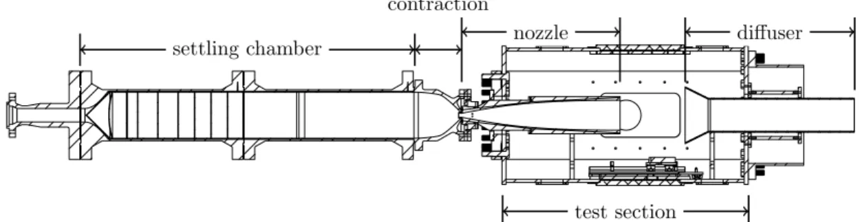
M6QT operates as a pressure-vacuum blowdown facility within the infrastructure at NAL. Figure 2.1 depicts the indoor tunnel flow path including the settling chamber (§ 2.1.3.1), nozzle (§ 2.1.3.2), test section (§ 2.1.3.3), and diffuser. Pressure and vacuum are supplied by way of a high-pressure air system a two-stage ejector system (§ 2.1.4).
settling chamber
contraction
nozzle
test section
diffuser
Figure 2.1: Cutaway of M6QT components.
Transition point Final expansion wave
Transition expansion wave Nozzle exit shock (overexpansion)
Quiet test core
Figure 2.2: M6QT nozzle annotated with the quiet test core (QTC) and associated features.
result of the significant expansion required to generate a hypersonic flow. The primary source of free-stream noise is acoustic waves radiating along Mach lines from the turbulent nozzle-wall boundary layer where the turbulent structures appear to the free stream as a rough wall. The problem of designing a hypersonic, low-disturbance wind tunnel is therefore one of maximizing the region of laminar flow on the nozzle wall. The quiet region of the flow is created when the Mach lines emanating from the transitional region of the nozzle-wall boundary layer meet at the nozzle centerline significantly downstream of the onset of uniform flow in the nozzle, resulting in a biconic region of quiet flow called the quiet test core (QTC, Figure 2.2).
RigimeshR conical flow spreader
RigimeshR dome flow spreader
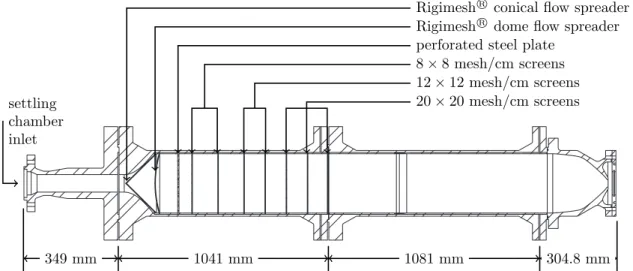
perforated steel plate 8×8 mesh/cm screens 12×12 mesh/cm screens 20×20 mesh/cm screens settling chamber inlet 349 mm 1041 mm 1081 mm 304.8 mm
Figure 2.3: M6QT settling chamber and contraction, annotated with internal features.
The following sections detail the layout of the tunnel and how they pertain to the creation of the QTC.
2.1.3.1 Settling chamber
The M6QT settling chamber (Figure 2.3) is separated into two sections. The first section, approximately 1 m in length, contains a series of flow conditioning features, including a conical Rigimesh® flow spreader and a dome Rigimesh® flow spreader to
encourage uniform flow entering the settling chamber, followed by a perforated steel plate and mesh screens of increasing mesh density to remove acoustic and turbulent fluctuations resulting from the upstream air flow path. The second section is empty and extends up to the contraction. These features provide a low-noise environment up to and entering the nozzle contraction and are the first step in generating a low-disturbance flow.
The entire settling chamber is heated externally by 8 kW of Ogden Mighty-Tuff electrical resistance heaters in order to maintain the settling chamber temperature at
1009.9 mm
190.3 mm 10.2 mm spacer
adjustable bleed gap throat diameter 25.4 mm
1009.9 mm
190.3 mm
10.2 mm spacer
adjustable bleed gap
throat diameter 25.4 mm
Figure 2.4: M6QT nozzle dimensions and detail. Inset is a close-up of the throat and bleed gap.
430 K and reduce convective preheating times.
2.1.3.2 Nozzle
The remaining three features pertinent to the QTC are part of the contraction and nozzle sections of the tunnel (Figure 2.4). While the flow quality features in the settling chamber help maintain a low-disturbance free-stream, minimizing the initial amplitudes generated by the receptivity process at the throat, the existing turbulent boundary layer in the settling chamber still contaminate the nozzle wall boundary layers in a conventional tunnel. In order to prevent this, M6QT includes a suction slot just upstream of the throat formed by the protrusion of the nozzle throat slightly into the contraction (Figure 2.4 inset). The bleed slot is connected to the vacuum in the diffuser and the turbulent boundary layer is sucked out of the tunnel prior to the throat, allowing a new, laminar boundary layer to form just upstream of
the throat. The low-disturbance free stream in the settling chamber combined with a highly polished nozzle surface minimizes the receptivity process in the incipient nozzle boundary layer.
Supersonic nozzles necessarily feature highly concave surfaces, and the transition process is therefore dominated by the Görtler instability. While the concave curvature cannot be avoided, the growth of the instability can be delayed by incorporating a long-expansion design. To this end the M6QT nozzle is substantially longer than a typical supersonic nozzle of the same Mach number, featuring an extended straight-wall section and pushing the onset of the concave surface farther downstream. This approach delays the growth of Görtler vortices and, therefore, the onset of turbulence in the boundary layer (Chen et al., 1993).
2.1.3.3 Test section
The M6QT is configured as a free jet wind tunnel featuring a sizable test section and less-intrusive probing mechanisms (Figure 2.1). The four long sides of this test section include modular access panels that can be used to support a variety of instrumentation and model configurations. In a typical configuration, the two side walls are outfitted with quick-release doors with optical access, the bottom panel is fitted with the model-mounting system and traverse mounting hardware and the top panel is simply closed. Other configurations have included a ceiling-mounted traverse and probe supports attached to the walls. Windows are available for both the visible and infrared portion of the spectrum depending on the application.
2.1.4 Infrastructure
The M6QT facility as is installed at the TAMU National Aerothermochemistry Laboratory (TAMUNAL) where it shares pressure-vacuum infrastructure with several
additional supersonic and hypersonic facilities. High pressure air is provided by a pair of CompAir 5442, each with a pumping capacity of 3.68 m3/min. (130 SCFM)
at 20.68 MPa (3000 psig). The compressed air is filtered with a pair of 99% efficient sub-micron particle filters and dried to a dew point of ≤ −40◦C by a twin-tower desiccant drier before being stored in an 23.2 m3 (820 ft3) tank at 17.24 MPa
(2500 psig).
The vacuum for the pressure-vacuum tunnels is generated using a two-stage Venturi air ejector. This system uses approximately 20 kg/s of compressed air at 1033 kPa while in operation and is capable of supplying a back pressure of as low as approximately 500 Pa to the wind tunnels. This high mass-flow requirement is the dominant factor in determining the tunnel run time.
The same compressed air reservoir supplies air for the tunnels. Prior to reaching the settling chamber, the air is heated by a 500 kW Chromalox electrical-resistance heater to achieve the desired total temperature (maximum 533 K) and re-filtered using 1-µm particle filter immediately prior to entering the tunnel. While in operation,
the M6QT draws approximately 1 kg/s of compressed air through the test section. The air requirements of the ejector and nozzle combined result in a maximum run time of approximately 50 seconds.
The M6QT shares this infrastructure with the Adaptively-Controlled Expansion (ACE) tunnel (Semperet al., 2009) in a parallel installation. In order for each tunnel to run separately from one another and while work continues in the other facility, they must each be capable of being isolated from the flow path when not in use. Each tunnel is thus isolated from the high-pressure air using a ball valve just downstream of the final particle filter and from the ejector system using a pneumatic knife gate valve just downstream of the diffuser.
508 mm 38.1 mm 116.8 mm R0.05 mm Pressure ports (×29) Type-K thermocouples (×51)
Figure 2.5: Diagram of the LaRC 93-10 flared cone. The first 8 pressure ports have an axial spacing of 25.4 mm on the forebody before transitioning to a 12.7 mm spacing. The first 8 thermocouples have the same spacing before transitioning to a 6.35 mm spacing.
2.2 Test models
The present experiments were performed using two wind tunnel models. The first, the NASA Langley 93-10 flared cone, was brought to Texas A&M along with the M6QT (§ 2.2.1). The second of these models, the TAMU 7DC, was recently designed at Texas A&M (§ 2.2.2). Each of these models has multiple roughness configurations including a smooth surface and roughness either in the form of azimuthally-periodic discrete roughness elements (DRE) or distributed roughness (§ 2.2.3).
2.2.1 Flared cone
The NASA Langley 93-10 flared cone (Figure 2.5) is the same model used in Lachowicz & Chokani (1996), Doggett & Wilkinson (1997), Horvath et al. (2002), and Hofferth (2013). Its profile consists of a right-circular cone with a 5◦ semi-vertex angle for the first 254 mm (10 in) of axial length at which point a flare with a constant radius of 2.36 m (93.071 in) begins and continues for an additional 254 mm (axially) to a total axial length of 508 mm (20 in). While tangency is maintained in the transition to the flare, radius of curvature is discontinuous. The adverse pressure
430 mm 155 mm 105.6 mm R0.05 mm Type-K thermocouples (×10)
Figure 2.6: Diagram of the TAMU 7DC right-circular cone.
gradient introduced by the flare promotes the growth of the second-mode waves, producing larger second-modeN-factors than on a 5◦ right-circular cone of equivalent length.
The model model is constructed of thin-walled stainless steel with a nominal thickness of 1.8 mm. The model includes removable tips comprising the first 38 mm of its length. While a variety of blunt tips are available, tip bluntness is known to stabilize a boundary layer and a sharp tip was used for the present study. The sharp tip has a specified tip radius of 2.54 µm.
The model is instrumented with both a series of pressure ports and type-K thermocouples along two rays separated by 180◦ of azimuth. Along one ray is a series of 29 pressure ports (21 of which are in the flared section) of 1 mm diameter. These ports are unused in the present study as the length of tubing required gives insufficient frequency response. Along the opposing ray are 51 thermocouples (43 along the flare) welded to the interior wall so as not to introduce roughness to the surface. The wall thickness at the thermocouple locations is 0.8 mm. The thermocouples are sampled once at each measurement location in order to monitor the wall temperature during each run.
2.2.2 Straight cone
The sharp-tipped, 7◦ right-circular cone has been adopted as the canonical geom-etry for high-speed crossflow studies and was therefore chosen for the present study. The Texas A&M 7-degree Cone (TAMU 7DC) was designed in house out of 17-4 PH stainless steel and has a total length of 430 mm (16.92 in.) from the sharp tip to the base. The model was designed as a two-piece model including a detachable tip comprising the first 155 mm (6.10 in.) and a conic frustum for the remainder of the length (Figure 2.6).
The large size of the removable tip offers several advantages over the more traditional small tips such as those on the LaRC 93-10 flared cone:
• The downstream axial location of the interface is further removed from the receptivity region of the model, minimizing the potential adverse effects of the interface on the stability of the boundary layer.
• The larger volume of the tip facilitates the future design of tips instrumented with active elements such as plasma actuators or suction/blowing slots in addition to the more standard tip bluntness or external roughness.
• The large-diameter threaded post can be keyed to fix its orientation and is large enough to be held in place easily from the inside using a nut rather than relying solely on threads in the tip of the frustum.
The interface between the tip and the frustum includes an O-ring to prevent any leakage flow as a result of any pressure difference between the inside of the cone and the free stream.
The frustum is a hollow, thick-walled model and is instrumented with 10 type-K thermocouples along its length spaced at 25.4 mm along the surface of the frustum.
While the thin-walled LaRC 93-10 typically reaches its adiabatic condition rather quickly, the TAMU 7DC, owing to its much larger thermal mass, does not. To combat this effect, the cone can be fitted with an internal heating system to bring its temperature to it’s adiabatic wall temperature and allowing the model to be held at a constant temperature during a run. In order to monitor the wall temperature during a run, the output from the thermocouples is averaged and provided to the PID process controller operating the model heaters.
2.2.3 Roughness configurations 2.2.3.1 Discrete roughness elements
Artificial roughness was created using high-temperature vinyl water slide decals. These decals involve screen-printing a UV-cured vinyl onto a dextrose backing and can be made in nearly any shape. The minimum decal thickness is approximately 3 µm and the maximum thickness used in the present work is approximately 20 µm,
though decals upward of 200 µm are theoretically possible. These decals are wetted
and placed on the surface of the model, at which point they can be easily slid into place and manipulated without the risk of damaging the elements. They are then allowed to dry overnight. The resulting decal roughness elements are durable and the surface may easily be cleaned by wiping with a damp towel or the elements may be removed with acetone.
2.2.3.2 Distributed roughness
Distributed roughness was created by combining 36-grit aluminum oxide abrasive blasting media with Duralco 4525 high-temperature epoxy. The resulting composite material adheres readily to metallic surfaces and is resistant to running on both
vertical and inverted surfaces, which are important qualities for application to the surface of the cone. The applied mixture can be spread on a surface in a layer that averages approximately 500 µm in thickness. Therefore, a depression of this depth
was machined into the cone surface prior to application of the rough composite in order that the average height of the rough surface was approximately equal with the cone surface. 10−3 10−2 10−1 100 101 102 10−5 10−3 10−1 101 103 105 λ[mm] PSD [ µ m 2 · mm]
Figure 2.7: A typical power spectrum across the composite distributed roughness.
The final surface roughness can be controlled by adjusting the grit size and grit-to-epoxy ration. In the present case, the rms roughness was measured to be approximately Rq ≈150 µm. The power spectral density of the roughness indicates
that energy is concentrated largely in wavelengthsλ >0.5mm with a roughly uniform, monomial decrease in power toward shorter wavelengths (Figure 2.7). The most
amplified azimuthal wavelength in the present experiments is expected to be m = 50, which, in the region of roughness, translates to approximately0.5mm ≤λ ≤1.5 mm.
2.3 Traversing system
2.3.1 Design considerations
All previous experiments performed in M6QT at Texas A&M utilized a two-axis probe traversing mechanism. These previous experiments focused exclusively on two-dimensional waves or free-stream measurements and were adeptly handled by the two-axis system. However, the limitations of this system prevented the study of three-dimensional phenomena. It was limited to wall-normal (or axis-normal) boundary-layer profiles along a given ray of a cone. For this reason, the development of a three-axis traversing mechanism was a key challenge in enabling the study of three-dimensional phenomena.
There were several parameters about which this new design was based. It must have three axes of motion, it must support axisymmetric models, it must support both flared cones and standard cones, and it must be able to function on models placed at nonzero angle of incidence to the flow.
While the requirement of three axes was obvious, the choice of coordinate system was not. The cheapest option would be to simply add a third z axis to the existing x-y traverse used in previous studies. Such a Cartesian system would be capable of measurements on a full half of an axisymmetric model, but would require a means of rotating the hot-wire probe to remain parallel to the surface and complicated adjustments to the probe to support nonzero angle of incidence. Given that all future plans involve axisymmetric models, a more natural choice of coordinate systems is cylindrical coordinates. Further, making the coordinate system co-axial with the model ensures that the system supports the angle of incidence requirement by default.
Figure 2.8: Three-dimensional traversing mechanism affixed to 7◦ cone model.
Several such traversing mechanisms have been designed and used in related studies at facility such as NASA Langley and Notre Dame (Corke et al., 2002; Schuele et al., 2013), which are fixed to the cone shaft and slide along the cone body. These systems, however, are unsuitable for use with flared cone models and their use as a template is limited. Instead, the final design features a two-axis “z-r” (axial-radial) traverse mounted to a carriage that moves around the model in the θ-direction (azimuth) using a rack and pinion gear system (Figure 2.8).
2.3.2 Design details 2.3.2.1 Ring structure
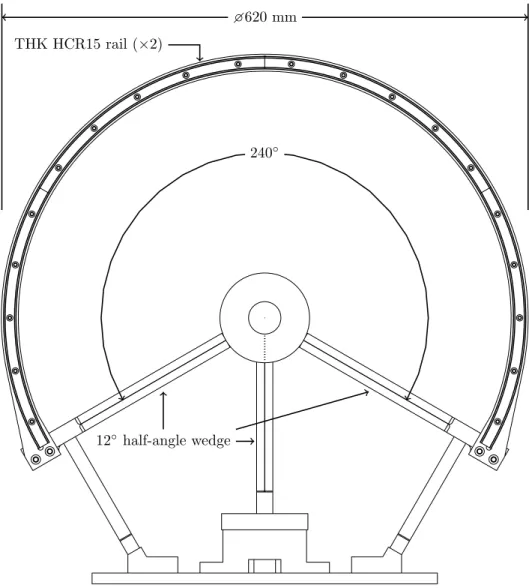
Figure 2.9 and Figure 2.10 depict the traverse with the carriage removed from the front and side respectively. The θ motion was constrained using a pair of THK HCR15-series motion guide systems. Each rail consists of 4 segments, each spanning 60◦, whose ends are ground to match and provide a seamless transition from one to the next. Each of these tracks was affixed to a 17-4 PH stainless steel structural arc with outer diameter 620 mm. These rings are affixed to the two “wing” structures extending from the cone axis such that the tracks face opposing directions. The rings are held rigid at a constant separation using a series of adjustable, threaded tie rods.
The wing supports connect to the support arcs and the model mounting system. As they are one of only two portions of the device to be exposed to the flow, they feature a12◦ half-angle wedge cut into their upstream side and a20◦ half-angle wedge affixed to the downstream side. The wings are supported near their ends with steel plates that connect them rigidly with the floor of the mounting system.
The aft support arc also supports the rack gear. The module 0.8 gear has a pitch diameter of 612 mm and the full ring included 765 teeth with a 20◦ pressure angle. It was initially machined as a disc, at which point the center was machined out to form a ring, and a 120◦ arc was removed to match the inside of the support arc. The matching pinion gear is affixed to the carriage and used to control the azimuthal motion (Figure 2.11).
THK HCR15 rail (×2)
12◦ half-angle wedge
620 mm
240◦
Figure 2.9: Cylindrical traverse system with the carriage removed (front view).
2.3.2.2 Carriage and motion stages
The carriage system (pictured in Figure 2.12), houses all three motors and the motion guides for the r- andz-axes. The carriage was constructed of many individual pieces, many of them designed to be rapidly cut from a single plate of steel on a wire EDM machine. This approach lends a great deal of modularity to many of the components, facilitating any future modification.
THK HCR15 rail (×2)
rack gear (module 0.8, 765 teeth, cut ring) adjustable tie rods
110 mm
Figure 2.10: Cylindrical traverse system with the carriage removed (side view).
Each axis utilizes a Faulhaber brushless DC servomotor with a built-in absolute encoder for its motion. The radial stage (r) uses a Faulhaber 2232S024BX4 AES-4096 motor while the azimuthal (θ) and axial (z) stages each use a Faulhaber 2250S024BX4 AES-4096 motor. Ther and z stages each have a ball screw with 1 mm lead coupled to their motors for a movement resolution of 244 nm per encoder line at an accuracy of ±5 lines. The θ stage features a roughly 246:1 planetary gearhead to provide substantial torque on the pinion gear, resulting in a movement resolution of 3◦×10−5
per encoder line and a±10line accuracy. The accuracy windows are adjustable within the Faulhaber MCBL 3006 S AES RS controllers, however these values represent the maximum degree of accuracy while still ensuring stable operation. These target
pinion gear (module 0.8, 65 teeth)
rack gear (module 0.8, 765 teeth, cut ring) radial-stage motor
azimuthal-stage motor axial-stage motor
Figure 2.11: Close-up view of the carriage and ring assembly and gear orientation.
Axis Range Min. step Accuracy
r 100 mm (max.) 2.5 µm ±1.22 µm
θ 220◦ 3◦×10−4 ±3◦×10−4
z 130 mm 2.5 µm ±1.22 µm
Table 2.1: Motion specification and details for the azimuthal traversing system
windows also determine the minimum step size. The specifications for this system are summarized in Table 2.1.
Figure 2.13 and Figure 2.14 depict the carrage from the front and side respectively. The azimuthal motor and pinion gear are attached to the top of the traverse using a set of adjustable screws and springs in order to provide adjustable contact force against the rack. Proper contact minimizes gear backlash and is checked prior to each wind tunnel run. The THK HCR15-series motion carriages affix to the inner sides of the two wall plates and the remainder of the interior space is used to provide room for the radial motor as it moves axially.
Figure 2.12: Isometric view of the carriage housing the motion stages.
The underside of the carriage includes a pair of THK HSR15-series linear motion guides, each with a pair of motion carriages to provide axial motion of the probe. A steel plate is mounted to the carriages. The radial stage is guided by a pair of THK RSR7 linear motion guides mounted to this plate along with the radial motor and ball screw.
The radial stage consists of several components. The first is a mounting block that attaches directly to the motion guides and ball screw and includes a channel used to mount the portion of the probe arm that will be exposed to the free stream. The system is designed to accommodate any number of probe designs so long as the
THK RSR7 rail/carriage (×2)
Axial motor and THK MTF 0601 ball screw/nut 142 mm
133.7
mm
Figure 2.13: Traverse carriage and radial arm (front view).
upper portion matches the two holes in the mounting block. Two set screws on either side of this channel hold the probe arm in place.
The probe arm is exposed to the flow and features two parts: a wedged body and an adjustable probe holder. The probe holder fits into a groove on the bottom of the arm and pivots around a large screw just aft of the wedge. The holder includes a series of holes that line up with corresponding holes in the probe arm through which small screws can be inserted to set a probe angle. The holder is once again held in place rigidly by two set screws on either side. The probe holder can support any number of probe types, including hot-wire or Pitot probes as long as their shape is such that an adapter can be built to fit the circular mount.
pinion gear radial-stage motor azimuthal-stage motor axial-stage motor THK HSR15 rail (×2) THK HSR15 carriage (×4) 12◦ half-angle wedge interchangeable probe THK MTF 0601 ball screw/nut adjustable probe mount THK HCR15 carriage (×4)
320 mm
Figure 2.14: Traverse carriage and radial arm (side view).
The system is controlled by three Faulhaber MCBL 3006 S AES RS motor controllers installed in a custom 24 VDC control cabinet with a linear power supply to eliminate the electronic noise inherent in switching power supplies. The controllers are operated from a purpose-built LabVIEW VI with GUI control panel that handles all motion control and data acquisition functions (§ 2.4).
2.4 Instrumentation and data acquisition system
Data acquisition (DAQ) is performed using two separate DAQ computers equipped with National Instruments (NI) hardware and software. DAQ processes are coordi-nated using custom-designed LabVIEW VIs.
One of these systems, “NALDAQ”, handles nearly all DAQ operations for general tunnel operating parameters for both hypersonic facilities installed at the lab including M6QT. The measured quantities handled by NALDAQ include temperatures and pressures at various stages along the ejector and tunnel air supply systems and the pressures at various stages along the tunnel flow path such as settling chamber temperature and pressure, test section pressure and diffuser pressure as well as M6QT bleed valve position and a host of other quantities. These quantities are sampled using an NI USB-6255 M Series 16-bit multiplexing DAQ board with 40 differential input channels at 1 kHz. These data are then averaged to 10 Hz and saved in a spreadsheet for each run cataloging ejector and tunnel performance. This system also displays the same data in a realtime monitoring mode when not acquiring and handles data for compressor status and storage tank pressure and is programmed to alert tunnel operators via SMS to changes in status of the high-pressure air system such as a full tank or compressor warnings and faults.
Pressures and temperatures handled by NALDAQ that are not critical to M6QT experimental analysis are measured using generic pressure and temperature sensors, typically Omega-brand pressure transducers and type-K thermocouples. Tunnel-critical pressures are handled with more sophisticated equipment. The settling chamber pressure is measured with an MKS Batatron 615A High-Accuracy Capaci-tance Manometer with a 10,000 torr full range and an MKS 670B signal conditioner. This system is temperature compensated and is quoted to be accurate to±0.2% of