Air Force Institute of Technology
AFIT Scholar
Theses and Dissertations Student Graduate Works
3-1-2018
Computational Investigation Using Bleed as a
Method of Shock Stabilization
Dayle L. Chang
Follow this and additional works at:https://scholar.afit.edu/etd
Part of theAerospace Engineering Commons, and theMechanical Engineering Commons
This Thesis is brought to you for free and open access by the Student Graduate Works at AFIT Scholar. It has been accepted for inclusion in Theses and Dissertations by an authorized administrator of AFIT Scholar. For more information, please [email protected].
Recommended Citation
Chang, Dayle L., "Computational Investigation Using Bleed as a Method of Shock Stabilization" (2018).Theses and Dissertations. 1763.
Computational Investigation Using Bleed as a Method of Shock Stabilization
THESIS
Dayle L. Chang, First Lieutenant, USAF AFIT-ENY-MS-18-M-247
DEPARTMENT OF THE AIR FORCE AIR UNIVERSITY
AIR FORCE INSTITUTE OF TECHNOLOGY
Wright-Patterson Air Force Base, Ohio
DISTRIBUTION STATEMENT A
AFIT-ENY-MS-18-M-247
COMPUTATIONAL INVESTIGATION USING BLEED AS A METHOD OF SHOCK STABILIZATION
THESIS
Presented to the Faculty
Department of Aeronautics and Astronautics Graduate School of Engineering and Management
Air Force Institute of Technology Air University
Air Education and Training Command in Partial Fulfillment of the Requirements for the Degree of Master of Science in Aerospace Engineering
Dayle L. Chang, B.S. Aerospace Engineering First Lieutenant, USAF
28 March 2018
DISTRIBUTION STATEMENT A
AFIT-ENY-MS-18-M-247
COMPUTATIONAL INVESTIGATION USING BLEED AS A METHOD OF SHOCK STABILIZATION
THESIS
Dayle L. Chang, B.S. Aerospace Engineering First Lieutenant, USAF
Committee Membership:
Major Darrell S. Crowe, PhD Chair
Dr. Scott E. Sherer Member
Lieutenant Colonel Jacob A. Freeman, PhD Member
AFIT-ENY-MS-18-M-247
Abstract
The interaction between shocks and the boundary layer in supersonic flow present difficulties in many applications such as inlet, aircraft, missile, and wind tunnel de-signs. These shock-wave/boundary layer interactions (SWBLI) frequently produce undesirable dynamic loads and separated unsteady flows, adversely impacting the performance and structural integrity of supersonic vehicles. Computational fluid dy-namics (CFD) is a successful tool in experimental planning and shows promise as a critical tool in understanding SWBLI. The goal of this research is to demonstrate the effect of bleed holes on shock stability using the OVERFLOW CFD solver to inform the planning of an Air Force Research Laboratory (AFRL) SWBLI wind tun-nel experiment. First, a two-dimensional, flat plate, single-hole configuration was developed. Massflow discrepancies of 14.8% were initially observed but reduced to 0% by analyzing the internal flow interaction with the boundary condition. Shock unsteadiness is then characterized using a canonical forward-facing step over a flat plate, which showed peaks at 5.8, 12.1, 31.2, 44.5, and 54.9 hertz. Though the fi-nal step of simulating bleed on the baseline forward-facing step was not achieved, promising time and frequency domain analysis techniques were demonstrated.
Acknowledgements
I cannot express enough gratitude for my research advisor and mentor, Major Dar-rell Crowe, who has helped see this project through to the end with encouragement, guidance, and freedom in the research. I also thank Dr. Scott Sherer, thesis commit-tee member and technical advisor, for his help getting me started with this project and Lieutenant Colonel Jacob Freeman for the learning opportunity he has provided as the third committee member. This work would not have been possible without the sponsorship of Dr. Mike Stanek. I thank Dan Galbraith and David Weston for their time and technical expertise answering my endless OVERFLOW questions. I thank my supervisors over the years: Charlie Tyler, Major Mark Gabbard, Major Christopher Terpening, and Larry Leny. They have given me tremendous support and flexibility during the pursuit of this research. I extend special thanks to Kirk Lawson, Jerry Trummer, and Matt Grismer for their faithful Mac and Linux admin-istrative help. I am grateful to both ASPRQ and the High Performance Computing Center for their endless computing hours, without which this research could not have been possible. Nobody has been more important to me during this research than my wife, to whom this is dedicated.
Table of Contents
Page
Abstract . . . iv
Acknowledgements . . . v
List of Figures . . . viii
List of Tables . . . xi
List of Symbols . . . xiii
List of Abbreviations . . . xv I. Introduction . . . 1 1.1 Motivation . . . 1 Peak Heating . . . 1 Dynamic Loads . . . 2 Unsteady Flow . . . 3 Current Views . . . 4 1.2 Research Objectives . . . 5
II. Background and Theory . . . 8
2.1 Derivation of the Navier-Stokes Equations . . . 8
Conservation Law within a Control Volume . . . 9
Conservation of Mass . . . 10
Conservation of Momentum . . . 10
Conservation of Energy . . . 12
Closing the Equations . . . 14
Integral Form of the Navier-Stokes Equations . . . 16
Differential Form of the Navier-Stokes Equations . . . 17
2.2 Boundary Conditions . . . 19
No-Slip Wall . . . 20
Supersonic Inflow . . . 21
Supersonic Outflow . . . 22
Specified Pressure Outflow . . . 23
Periodic . . . 23
2.3 Turbulence Modeling . . . 24
Reynolds-Averaged Navier-Stokes Equations . . . 25
Spalart-Allmaras Turbulence Model (Negative Form) . . . 27
Large Eddy Simulation and Detached Eddy Simulation . . . 31
Delayed Detached Eddy Simulation . . . 32
Page
III. Methodology . . . 36
3.1 Grid Generation . . . 36
Chimera Grid Tools . . . 36
Pegasus . . . 37
3.2 Flow Solver . . . 37
3.3 Bleed Flow Analysis . . . 38
Mayer and Paynter Model . . . 38
Davis Model . . . 40
Slater Model . . . 41
Previous Experimental Results . . . 46
Previous Computational Results . . . 46
IV. Results and Analysis . . . 49
4.1 Three-Dimensional Wind Tunnel Model . . . 49
4.2 Two-Dimensional Plenum Outflow Verification . . . 55
Grid Resolution and Patch Sizing Study . . . 56
Specified Pressure Boundary Condition Comparison with Physical Ducting . . . 72
Removing Boundary Condition Effects with Complete Suction . . . 79
4.3 Shock Unsteadiness Characterization . . . 82
Determining the Correct Mesh Topology and Flow Parameters . . . 82
Analysis of Shock Unsteadiness . . . 86
V. Conclusion . . . 90
Appendix A. Source Code . . . 92
1.1 MATLAB Slater Calculations . . . 92
1.2 TCL Code . . . 93
1.3 Fortran Code . . . 108
Bibliography . . . 112
List of Figures
Figure Page
1 Supersonic tunnel model on a support sting. . . 5 2 Data from Willis et al. [41] normalized by the total
pressure at the boundary layer edge [31] . . . 35 3 Data from Willis et al. [41] normalized by the bleed
surface static pressure [31] . . . 43 4 The Slater model compared to other experimental data
sets . . . 44 5 Sonic flow coefficients for bleed flow through a single
bleed hole [29]. . . 48 6 Errors in the mesh during the hole-cutting process . . . 51 7 Visualizations of bleed flow within the
three-dimensional wind tunnel model simulation . . . 53 8 Quadratic fit of the massflow through the wind tunnel
model bleed hole at various pressure ratios and
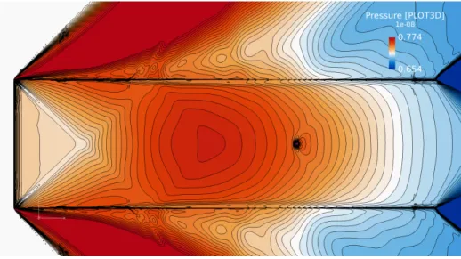
compared to the Slater model. . . 54 9 Pressure contour of the wind tunnel model along the
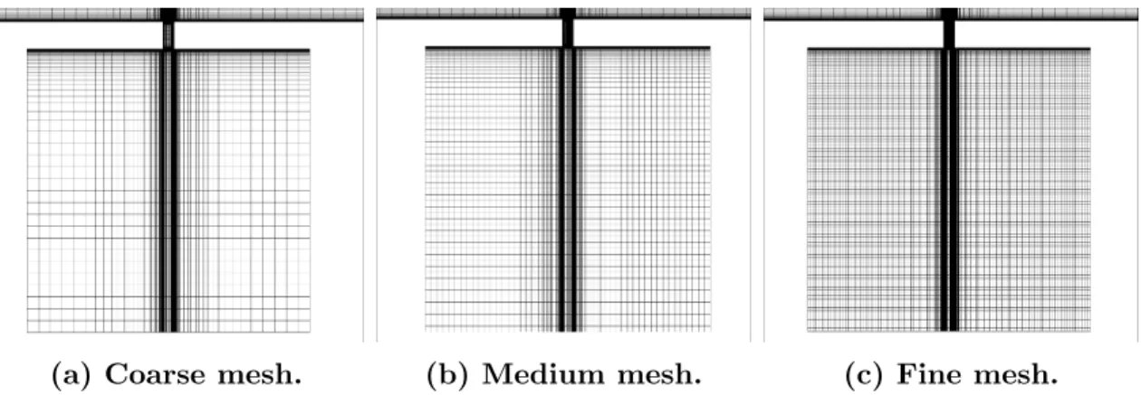
surface. . . 54 10 Grid spacing in the plenum with the patch sizing overlaid. . . 57 11 Mesh visualization of the three mesh refinement levels
in the plenum. . . 58 12 Verification of the computational simulation with
experimental parameters. . . 60 13 Residual history of the small specified pressure patch for
various grid refinement levels. . . 61 14 Residual history of the medium specified pressure patch
for various grid refinement levels. . . 62 15 Residual history of the large specified pressure patch for
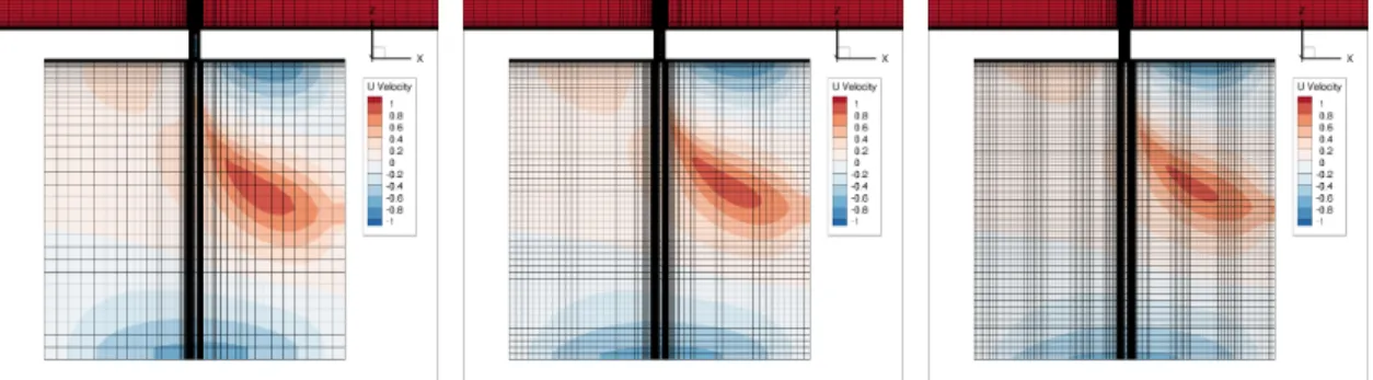
Figure Page 16 Contours of u-velocity and streamlines for the small
patch. . . 64 17 Contours of u-velocity and streamlines for the medium
patch. . . 64 18 Contours of u-velocity and streamlines for the large
patch. . . 65 19 Massflow behavior with the small specified pressure
patch at various points in the plenum for various grid
refinement levels. . . 66 20 Massflow behavior with the medium specified pressure
patch at various points in the plenum for various grid
refinement levels. . . 67 21 Massflow behavior with the large specified pressure
patch at various points in the plenum for various grid
refinement levels. . . 68 22 Key features of the flow structure within the bleed hole. . . 70 23 Contours of Mach number and streamlines of both slip
and no-slip plenum walls using the small-width duct. . . 73 24 Massflow behavior of the small-width duct at a pressure
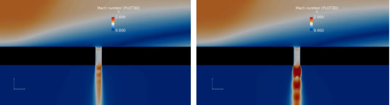
ratio of 0.25. . . 74 25 Contours of Mach number and streamlines of both slip
and no-slip plenum walls using the medium-width duct. . . 74 26 Massflow behavior of the medium-width duct at a
pressure ratio of 0.25. . . 75 27 Contours of Mach number and streamlines of both slip
and no-slip plenum walls using the large-width duct. . . 76 28 Massflow behavior of the large-width duct at a pressure
ratio of 0.25. . . 77 29 Contours of Mach number and streamlines of the
large-width inviscid duct for various plenum pressure
Figure Page 30 Streamlines and Mach number contours for the
complete plenum suction simulation. . . 79 31 Sonic coefficient plot of the two-dimensional simulation
using complete suction compared to the Slater model. . . 80 32 Mach number contour using the SA turbulence model. . . 84 33 Inadequately resolved shock structure using DES. . . 85 34 Non-physical simulation using DES due to lack of
span-wise three-dimensional turbulence relief. . . 86 35 Grid refinement system around the forward-facing step. . . 87 36 Simulation of an adequately resolved DES shock
structure. . . 88 37 Time history of pressure at locations 1 inch apart 0.5
inches above the surface. . . 89 38 FFT displaying frequency content of the pressure time
List of Tables
Table Page
1 Closure Constants for the Negative SA Turbulence Model . . . 31
2 Coefficients for the Davis scaled empirical model as a function of Mach number [11]. . . 40
3 Coefficients for the Davis scaled empirical model as a function of the plenum pressure ratio [11]. . . 41
4 Coefficients for the quadratic fit of the Slater model . . . 44
5 Reference conditions at the boundary layer edge and 2.46 inches ahead of the bleed hole center used in the Slater computational simulation [30] . . . 46
6 Mesh parameters for the three-dimensional wind tunnel model in freestream flow . . . 50
7 Flow simulation parameters for the tunnel model in freestream air. . . 51
8 Differences in the massflow in and out of the plenum, where nominal pressure ratio is the ratio between the plenum pressure and the freestream pressure. . . 55
9 Boundary layer parameters from experiment [6]. . . 56
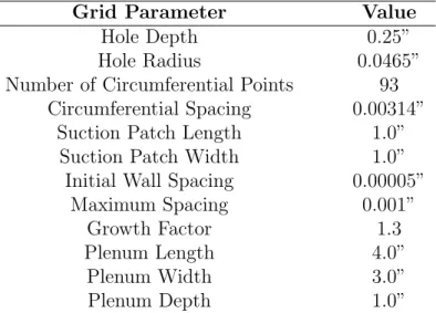
10 Mesh parameters and physical dimensions. . . 58
11 Mesh dimensions for the grid refinement study. . . 58
12 Flow simulation parameters for the tunnel model in freestream air. . . 59
13 Percent difference of the steady-state inflow massflow rate coefficients in the plenum with the overall mean. . . 69
14 Percent difference of the steady-state outflow massflow rate coefficients in the plenum with the overall mean. . . 69
15 The qualitative oscillatory behavior and accuracy of massflow rates as a function of mesh refinement and patch sizing summarized. . . 71
Table Page 16 Percent difference of the steady-state inflow massflow
rate coefficients in the plenum with the overall mean
compared with complete suction. . . 81 17 Percent difference of the steady-state outflow massflow
rate coefficients in the plenum with the overall mean
compared with complete suction. . . 81 18 The qualitative oscillatory behavior and accuracy of
massflow rates as a function of mesh refinement and patch sizing with the results from complete suction
summarized. . . 81 19 Mesh dimensions for the four grid system modeling the
forward-facing step. . . 83 20 Flow parameters for the forward-facing step. . . 83
List of Symbols
Symbol Page
Ω control volume . . . 9
dΩ differential control volume . . . 9
κ thermal diffusivity coefficient . . . 9
ρ density . . . 9
~v velocity vector . . . 9
~n outward-facing unit normal vector . . . 9
Sv volume source . . . 9
~ Ss surface source vector . . . 9
dS differential surface element . . . 9
Fd diffusive flux tensor . . . 10
Fc convective flux tensor . . . 10
~ Sv volume source vector . . . 10
Ss surface source tensor . . . 10
I unit tensor . . . 11
p pressure . . . 11
τ viscous stress tensor . . . 11
E total energy . . . 12
k thermal conductivity coefficient . . . 12
T absolute static temperature . . . 12
µ dynamic viscosity . . . 13
λ second viscosity . . . 13
Symbol Page
v y-component of velocity . . . 14
w z-component of velocity . . . 14
P r Prandtl number . . . 15
~ Q vector of conserved variables . . . 16
~ Fc convective flux vector . . . 16
~ Fd diffusive flux vector . . . 16
µt eddy viscosity . . . 26
kt turbulent thermal conductivity . . . 26
˜ ν turbulent kinematic viscosity parameter (S-A) . . . 27
νt kinematic eddy viscosity . . . 27
ν laminar kinematic viscosity . . . 27
Q flow coefficient . . . 33
˙ m mass flow rate . . . 33
Φ bleed porosity . . . 33
A area . . . 33
pt total pressure . . . 34
List of Abbreviations
Abbreviation Page
SWBLI shock-wave/boundary layer interaction . . . 1
NASA National Aeronautics and Space Administration . . . 4
SBIR Small Business Innovation Research . . . 4
NHFRP National Hypersonics Foundational Research Plan . . . 4
AFOSR Air Force Office of Scientific Research . . . 4
RTO/AVT Research and Technology Office, Air Vehicle Technology . . . 5
NATO North Atlantic Treaty Organization . . . 5
AFRL Air Force Research Laboratory . . . 5
TGF Trisonic Gasdynamics Facility . . . 5
CFD computational fluid dynamics . . . 5
PDE partial differential equations . . . 19
DNS direct numerical simulation . . . 25
RANS Reynolds-averaged Navier-Stokes . . . 25
S-A Spalart-Allmaras . . . 27
LES large eddy simulation . . . 31
DES detached eddy simulation . . . 32
DDES delayed detached eddy simulation . . . 32
CGT Chimera Grid Tools . . . 36
TCL Tool Command Language . . . 36
GUI graphical user interface . . . 36
FOMOCO Force and Moment Computation . . . 36
Abbreviation Page HLLC Harten-Lax-van Leer-Contact . . . 59 SSOR Implicit Symmetric Successive Over-Relaxation . . . 59
COMPUTATIONAL INVESTIGATION USING BLEED AS A METHOD OF SHOCK STABILIZATION
I. Introduction
1.1 Motivation
Shock waves are a natural phenomenon that arise in supersonic operation. When the shock interacts with the boundary layer, the situation becomes complex and is an important design consideration for applications in transonic and supersonic flows. This interaction occurs so pervasively that it has been termed the shock-wave/boundary layer interaction (SWBLI). Successful utilization of aircraft, missiles, inlets, or wind tunnel designs in supersonic flow are contingent on the favorable behavior of the SWBLI in both internal and external flows [15]. Three key issues that arise due to SWBLI are identified by Holden: peak heating, dynamic loads, and effects of separated unsteady flows [16]. These three issues and their effects on practical applications are discussed in greater depth below and together represent the motivation for this research. The chapter concludes by summarizing the objectives of this research.
Peak Heating.
The severe effects of peak heating are well documented in SWBLI, particularly in hypersonic flows. Peak heating rates vary between 10 to 100 times the incom-ing boundary-layer flow and many times the equivalent stagnation point value [13]. Knight and Degrez note that “heat transfer distribution predictions are generally
poor, except for weak interactions, and significant differences are evident between turbulence models. . . of up to 100% between experiment and numerical results” [17]. These high temperatures cause localized stresses which affect practical designs factors such as geometry, fatigue, material selection, and thermal protection [13].
Dynamic Loads.
In many aeronautical applications, parameters of critical importance are imposed by unsteady conditions that can occur during flight, rather than steady conditions. Although these events are rare or do not contribute much to the local average energy, they can correspond to high local stress, which can affect the entire behavior of the system. In supersonic flows, an important case occurs when unsteadiness involves shock waves producing locally large pressure gradients. The pressure fluctuations impose strong aerodynamic loads which propogate downstream of the shock wave. This occurs in shock-induced separation, where low-frequency unsteadiness is pro-duced [23].
The impact of unsteady aerodynamic loading is seen in the controls response sys-tem of aircraft and missile bodies. High-speed, anti-armor, kinetic energy penetrators (Mach 4-8 at sea level) are configurations of interest to the U.S. Army that pose many simulation and experimental challenges due to the SWBLI. Following discharge from the gun, lateral thrusters or control surfaces may be used to guide and control such projectiles. Accurate characterization of the three-dimensional, unsteady, laminar, transitional, and turbulent interactions that sweep rapidly across the body is im-portant in ensuring proper aerodynamic control of aerodynamic bodies and requires accurate modeling of SWBLI [13].
Another example of the negative impact of unsteady aerodynamic loading is plume-induced boundary-layer separation in missile design. The boundary layer
sep-arates off the missile afterbody rather than at the base of the missile, resulting in a strong and adverse pressure gradient generated by the interaction of the expanding plume and surrounding freestream. The premature boundary layer separation gener-ates large, unsteady, and asymmetric loads on the missile body for which the control surfaces and response system must have adequate control authority and response tim-ing to overcome [13]. In the worst case, inadequate control authority or poor control respose may cause the control surfaces themselves to experience premature bound-ary layer separation, resulting in a partial to total loss of control effectiveness. An understanding of the fundamental flow physics allows for missile designs to success-fully demonstrate control authority during flight and achieve maximum performance. Shaw et al. notes this plume-induced separation feature is not unlike the SWBLI behavior on a compression ramp and shares many common features, which can be used to characterize the separation for missile applications [28].
Unsteady Flow.
Mixed compression inlets are designed to produce a shock train structure and terminal shock that allows for the highest total pressure recovery. However, these shocks are sensitive to flow disturbances and flow unsteadiness due to their interaction with the boundary layer. If the effects of unsteady flow are not mitigated, changes to the flow structure can displace the shock wave into a less efficient configuration. If the disturbances are large enough, the terminal shock may move upstream and ultimately out of the inlet, resulting in unstart that produces large transient forces on the airframe and cause engine surge [13].
Bleed holes are used as a method of active flow control to mitigate flow unsteadi-ness inside the inlet. By adjusting the mass-flow rate reaching the diffuser in response to perturbations in the engine operation or inlet flow, the shock train is stabilized.
The disadvantage of such a method is that energy and thrust is reduced while weight is increased. Factors such as bleed hole location, hole geometry, suction massflow rate, and many others make this an area of ongoing research [13].
Current Views.
SWBLI is recognized as a long-standing research area in the aerospace community, garnering wide attention both nationally and internationally [15]. A 1996 National Aeronautics and Space Administration (NASA) research announcement stated that “improved air-breathing engines will require a clearer understanding of the basic flow physics of propulsion system components.” The design of higher performance inlets and nozzles that are “quieter, shorter, lighter” requires “benchmark quality data for flowfields including shocks, boundary layers, boundary layer control, separation, heat transfer, surface cooling and jet mixing.” These areas all involve SWBLI in one form or another [13].
The NASA Small Business Innovation Research (SBIR) solicitation in 2015 em-phasized the need for basic research to be relevant for practical applications: “One of the greatest issues that NASA faces in transitioning advanced technologies into future aeronautics systems is the gap . . . between the maturity level of technologies developed through fundamental research and the maturity required for technologies to be infused into future air vehicles and operational systems” [21]. Fundamental re-search faces “inadequacies in our understanding of boundary layer turbulence [that] increase reliance upon a more qualitative, physics-guided approach to discovery” [20]. The National Hypersonics Foundational Research Plan (NHFRP) was developed by the Air Force Office of Scientific Research (AFOSR), NASA, and Sandia National Laboratory. This plan provides a framework of the main areas in hypersonics research of which SWBLI is a key component. The Research and Technology Office, Air Vehicle
Technology (RTO/AVT) has been an integral part of that development under North Atlantic Treaty Organization (NATO) [27].
Flow control for SWBLI remains a key issue for future technology vehicles but is regarded as a complicated and vexing problem. To make the proper trade-offs in design, a deep, physical understanding of the mechanisms of these interactions must be understood with both experimental and computational tools that are both robust and accurate [13].
1.2 Research Objectives
A supersonic wind tunnel model designed for research by the Air Force Research Laboratory (AFRL) (shown in Figure 1) will be used in an upcoming SWBLI experi-ment. The experiment will be conducted in the Trisonic Gasdynamics Facility (TGF) at Wright-Patterson Air Force Base and will explore various methods of understand-ing and mitigatunderstand-ing SWBLI. The first entry of the AFRL experiment will incorporate bleed holes towards stabilization of an unsteady shock as a first step towards the goal of understanding and mitigating SWBLI.
Figure 1. Supersonic tunnel model on a support sting.
a successful design tool in experimental planning and shows promise as a critical tool in understanding SWBLI [13, 42]. The current computational research will inform the planning and design of the AFRL experiment to save on tunnel run-time and to bring insight into the flow physics of the experiment. The goal of this research is to use CFD to demonstrate the effect of bleed holes on shock unsteadiness. Since the wind tunnel model currently does not incorporate a shock near the bleed hole in the experiment, the computational effort will use a canonical forward-facing step to generate the unsteady shock and this effort will determine if this configuration is a successful model for mitigating shock unsteadiness. The objectives of this research are listed below:
• Develop grid independent computational domains
• Compare against previous experimental and computational work
• Explore validity of using a two-dimensional bleed model to remove plenum ef-fects
• Characterize shock unsteadiness
• Demonstration of improved shock stability
To accomplish these objectives, this research will focus on characterizing the flow physics of a single bleed hole on a flat plate to ensure the flow is accurately mod-eled. Computational simulations of the bleed hole will be verified against other com-putational studies in addition to empirical models based on experimental data. A two-dimensional simulation was used for simplicity so the value of a two-dimensional assumption in modeling flow through a bleed hole, or slot in two dimensions, was examined. To assess an improvement in shock stability, a baseline shock was first characterized using a forward-facing step on a flat plate. Then, the change in shock
strength and unsteadiness could be quantified after incorporating a bleed hole ahead of the forward-facing step. More than demonstrating the quantitative improvements in shock stabilization, this research aims to yield insight and a computational frame-work into how high-fidelity CFD can assist in identifying areas of unsteadiness due to SWBLI as well as recommendations on how flow control is used to mitigate negative effects.
Chapter I introduces the subject, motivation, and objectives of this research. Chapter II presents further background information on SWBLI and flow control to include relevant research areas. In addition, it will provide fundamental theory for expected flow phenomena. Chapter III explains the computational methodologies used in the computational setup including grid generation, flow solver parameters, turbulence modeling, and the overall experimental approach. Chapter IV presents the results of the grid topology screening, time step and grid refinement study and aerodynamic characterization of the shock unsteadiness at supersonic conditions. The results are analyzed and compared to experimental data and empirical models. A summary of the research and recommendations for future work are given in Chapter V.
II. Background and Theory
2.1 Derivation of the Navier-Stokes Equations
The Navier-Stokes equations describe the motion of viscous fluids and are useful because they describe the physics of scientific and engineering interests. For example, they are used to model the weather, ocean currents, water flow in a pipe, and air flow around a wing. Before deriving the Navier-Stokes equations, assumptions about the flow are made and physical principles are discussed to arrive at the governing equations of fluid dynamics in the following sections.
The first assumption is that the density of the fluid is assumed to be high enough such that the flow is approximated as a continuum. This implies that an infinitesi-mally small, or differential, element of the fluid still contains a sufficient number of particles for which the mean velocity and mean kinetic energy can be specified. This assumption enables important quantities such as velocity, pressure, temperature, and density to be defined at each point in the fluid. In mathematical terms, the continuum assumption states the mean free path of molecules λ is proportionally much smaller than the characteristic length of interest L as shown below
kn =
λ
L 1 (1)
where kn is the Knudsen number. The derivation of the Navier-Stokes equations is
based on the fact that the dynamic behavior of the fluid is determined by the following conservation laws:
• Conservation of Mass
• Conservation of Momentum
The conservation of these flow quantities means that its total variation inside an arbitrary volume can be expressed as the net effect of the flux, or the rate a flow quantity crosses a boundary surface, any internal forces and sources, and external forces acting on the volume. The flux is decomposed into two parts: one due to convective transport and the other due to molecular motion present in the fluid at rest, or diffusion [5]. In the following discussion, the finite control volume is defined and a mathematical description of its physical properties for fluid flow is detailed.
Conservation Law within a Control Volume.
A control volume Ω is defined as an arbitrary and finite region of fluid flow fixed in space and bounded by the closed surface dΩ. The surface elementdS represents a small and finite portion of the surface dΩ and~n is the associated outward pointing unit normal vector. The net change of a fluid property within the control volume is determined by performing a balance between the net flow in and out of the control volume, such as the force or total energy exchange. This is expressed in a mathemati-cal sense: the change of a given property in time is described as the sum of convective fluxes, diffusive fluxes, volume sources, and surface sources in and through a control volume. This conservation law is shown for the general property U in integral form as shown below: ∂ ∂t Z Ω U dΩ = I ∂Ω [κρ(∇U∗·~n)−U(~v·~n)]dS+ Z Ω SvdΩ + I ∂Ω ~ Ss·~n dS (2)
where Ω is the control volume, dΩ is the differential control volume,κ is the thermal diffusivity coefficient, ρ is density, ~v is the velocity vector, ~n is the outward-facing unit normal vector, Sv is the volume source, S~s is the surface source vector, and dS
conservation law still holds and is further generalized in vector form as ∂ ∂t Z Ω ~ U dΩ = I ∂Ω h Fd−Fc ·~nidS+ Z Ω ~ SvdΩ + I dΩ Ss·~n dS (3)
whereFdis the diffusive flux tensor,Fcis the convective flux tensor,S~v is the volume
source vector, andSs is the surface source tensor. This formulation of conservation is
the basis of the derivation for the conservation laws of mass, momentum, and energy in the continuing discussion.
Conservation of Mass.
The law of conservation of mass states that mass can neither be created nor destroyed. Therefore, the time rate of change of mass within a given control volume is dependent only on the net mass coming in and out of the control volume due to convection. Simply put, convection is the only mechanism by which mass can change within a control volume. The diffusive flux, surface source, and volume source terms all go to zero as a result. This concept is expressed mathematically below:
∂ ∂t Z Ω ρ dΩ + I ∂Ω ρ(~v·~n)dS = 0 (4)
This yields the conservative, integral form of the continuity equation.
Conservation of Momentum.
The law of conservation of momentum states that the time rate of change of momentum is equal to the net force acting on a control volume. The momentum of an infinitesimally small portion of the control volume Ω is ρ~v dΩ, where~v = [u, v, w]T in a three component Cartesian coordinate system. The variation in time of momentum
within the control volume is described as ∂ ∂t Z Ω ρ~v dΩ (5)
The convective flux term is the transfer of momentum across the boundary of the control volume
− I
∂Ω
ρ~v(~v·~n)dS (6)
The diffusive flux term is zero since there is no diffusion of momentum for a fluid at rest. The volume sources for momentum conservation are called body forces and described as forces which act directly on the mass of the volume such as gravitational, buoyancy, Coriolis, centrifugal, or electromagnetic forces. They are ignored in this derivation by setting the sources equal to zero.
The surface sources for momentum conservation act directly on the surface of the control volume and consist of two components: the pressure distribution imposed by the fluid surrounding the volume, −pI, and the shear and normal stresses resulting from the friction between the fluid and the surface of the volume, τ, as shown below
Ss =−pI+τ (7)
where I is the unit tensor, p is pressure, and τ is the viscous stress tensor. Each of the terms are summed up in the following mathematical expression:
∂ ∂t Z Ω ρ~v dΩ + I ∂Ω ρ~v(~v ·~n)dS+ I ∂Ω p~n dS − I ∂Ω τ·~ndS = 0 (8)
Conservation of Energy.
The law of conservation of energy states that the internal energy of the control volume is equal to the rate of work performed on the volume and the net heat supplied to the volume. The conserved quantity is the total energy per unit volume ρE and its variation in time within the volume Ω is expressed as
∂ ∂t
Z
Ω
ρE dΩ (9)
Just like the previous mass and momentum equations, the convective flux term is specified as
− I
∂Ω
ρE(~v·~n)dS (10)
In contrast to the previous mass and momentum equations, the diffusive flux term is present in the energy equation and describes the diffusion of heat due to molecular thermal conduction. The diffusive flux term F~d is written in the form of Fourier’s
law of heat conduction, which characterizes heat diffusion as the heat transfer due to temperature gradients
~
Fd =−k∇T (11)
where k is the thermal conductivity coefficient and T is the absolute static tempera-ture.
The volume source for the energy equation is the volumetric heating due to the absorption or emission of radiation, or due to chemical reactions as well as work done by the body forces. These volume sources are ignored and not considered for this derivation.
and normal stresses on the fluid element
~
Ss=−p~v+τ ·~v (12)
where τ is the stress tensor
τ = τxx τxy τxz τyx τyy τyz τzx τzy τzz (13)
The off-diagonal elements of τ represent the viscous shear stresses and defined as
τxy =τyx =µ ∂u ∂y + ∂v ∂x τxz =τzx=µ ∂u ∂z + ∂w ∂x τyz =τzy =µ ∂v ∂z + ∂w ∂y (14)
The diagonal elements represent the viscous normal stresses and defined as
τxx =λ ∂u ∂x + ∂v ∂y + ∂w ∂z + 2µ∂u ∂x τyy =λ ∂u ∂x + ∂v ∂y + ∂w ∂z + 2µ∂v ∂y τzz =λ ∂u ∂x + ∂v ∂y + ∂w ∂z + 2µ∂w ∂z (15)
where µ represents the dynamic viscosity and λ represents the second viscosity. Stoke’s hypothesis eliminates λ by relating the second viscosity and the dynamic viscosity as a bulk viscosity, which represents the property that is responsible for energy dissipation in a fluid of uniform temperature during a change in volume at a finite rate as shown.
λ+2
The diagonal elements are then simplified using Stoke’s hypothesis (Equation 16) for the viscous normal stresses (Equation 15) as shown below
τxx = 2µ " ∂u ∂x − 1 3 ∂u ∂x + ∂v ∂y + ∂w ∂z # τyy = 2µ " ∂u ∂x − 1 3 ∂u ∂x + ∂v ∂y + ∂w ∂z # τzz = 2µ " ∂u ∂x − 1 3 ∂u ∂x + ∂v ∂y + ∂w ∂z # (17)
The terms are summed in the following mathematical expression: ∂ ∂t Z Ω ρE dΩ + I ∂Ω ρE(~v·~n)dS = I ∂Ω k(∇T ·~n)dS− I ∂Ω p(~v·~n)dS + I ∂Ω τ·~v·~n dS (18)
This yields the conservative, integral form of the energy equation.
Closing the Equations.
The mass, momentum, and energy equations are collectively referred to as the Navier-Stokes equations, representing a system of five equations in three dimensions for the five conserved variables ρ, ρu, ρv, ρw, and ρE. However, the governing equations contain nine unknown flow field variables: ρ, u, v, w, E, p, T, µ, and k. Therefore, four additional equations are needed to close the equations, which is accomplished by formulating thermodynamic relations between the two unknown state variables for pressure, p, and temperature, T. For an ideal perfect gas, the equation of state assumes the form
where R denotes the specific molecular gas constant. This equation can be written as a function of the conserved variables by using the definition of enthalpy
H =h+ |~v| 2
2 =E+
p
ρ (20)
which relates the total enthalpy to the total energy. Using the definitions
R=cp−cv, γ =
cp
cv
, h=cpT
the enthalpy equation (Equation 20) is substituted into the equation of state (Equa-tion 19) to obtain for the pressure as a func(Equa-tion of the conserved variables
p= (γ−1)ρ E− u 2+v2 +w2 2 (21)
Calculating temperature becomes trivial with the aid of Equation 19. Dynamic viscosityµis strongly dependent on temperature but only weakly dependent on pres-sure. Sutherland’s formula describes this relationship for air (in SI units)
µ= 1.45T 3 2 T + 110 ·10 -6 (22)
where the temperature, T, is in degrees Kelvin (K). The Prandtl number (P r) is a dimensionless number defined as the ratio of momentum diffusivity to thermal diffusivity
P r= cpµ
k (23)
The Prandtl number is assumed constant in the flow for air with a value of Pr =
0.72. Therefore, the thermal conductivity, k, is determined from temperature. [4, 5, 37–39].
Integral Form of the Navier-Stokes Equations.
For the complete system of the Navier-Stokes equations, Equations 4, 8 and 18 are combined using the general conservation law (Equation 3) into the following vectorized form: ∂ ∂t Z Ω ~ Q dΩ + I dΩ (F~c−F~v)dS = 0 (24)
where Q~ is the vector of conserved variables in three dimensions, F~c represents the
convective fluxes, and F~d represents the diffusive fluxes. Note that Equation 24 does
not include any source terms. These three vectors for the five total equations are defined as follows ~ Q= ρ ρu ρv ρw ρE (25) ~ Fc= ρV ρuV +nxp ρvV +nyp ρwV +nzp ρHV (26) ~ Fv = 0 nxτxx+nyτxy +nzτxz nxτyx+nyτyy+nzτyz nxτzx+nyτzy+nzτzz nxΘx+nyΘy+nzΘz (27)
where V is the contravariant velocity V ≡~v·~n =nxu+nyv+nzw (28) and where Θx =uτxx+vτxy+wτxz +k ∂T ∂x Θy =uτyx+vτyy +wτyz+k ∂T ∂y Θz =uτzx+vτzy+wτzz +k ∂T ∂z (29)
Equations 24 -29 ultimately describe the exchange of mass, momentum, and energy through the boundary dΩ of a fixed control volume Ω in what is known as the integral form of the Navier-Stokes equations.
Differential Form of the Navier-Stokes Equations.
Though not always the case, the integral form of the Navier-Stokes equations is better understood in the context of the finite volume method. However, the code used in this research (OVERFLOW) uses the finite-difference method and so the differential form of the Navier-Stokes equations is presented for completeness.
Recall the integral form of the Navier-Stokes equations were presented in the discussion from the starting assumption that the control volume was fixed in space, an Eulerian frame of reference. An alternative approach examines the differential element moving with the fluid flow, a Lagrangian frame of reference, rather than a control volume fixed in space. The two frames of reference are related through the Reynolds transport theorem which relates the rate of change of a system property within a fixed region (control volume) to the time derivative of a system property (differential element). Applying the theorem to the integral form of the governing
equations (Equation 24) leads to the differential form as shown below ∂ ∂t Z Ω ~ Q dΩ + Z Ω ∇·F~c−F~v dΩ = 0 (30)
The integral drops out for an arbitrary control volume Ω and the equation is written in the differential form as
∂ ~Q ∂t +∇· Fc−Fv = 0 (31)
It is typical to combine the convective and viscous fluxes and expand the gradient operator ∇ to arrive at the generalized form
∂ ~Q ∂t + ∂ ~E ∂x + ∂ ~F ∂y + ∂ ~G ∂z = 0 (32)
where E~, F~, and G~ represent the fluxes in the x-, y-, and z-directions, respectively, as shown below ~ Q= ρ ρu ρv ρw ρE (33) ~ E = ρu ρu2+p−τ xx ρuv−τxy ρuw−τxz (ρE+p)u−Θx (34)
~ F = ρv ρuv−τxy ρv2+p−τ yy ρvw−τyz (ρE+p)v−Θy (35) ~ G= ρw ρuw−τxz ρvw−τyz ρw2 +p−τ zz (ρE+p)w−Θz (36)
Equations 29 and 32 -36 describe the change in mass, momentum, and energy at an infinitesimally small element of the flow in what is known as the differential form of the Navier-Stokes equations.
2.2 Boundary Conditions
The Navier-Stokes equations are a set of partial differential equations (PDE) for which an analytical solution does not currently exist, but can be solved approximately and iteratively using computers. In computing solutions to PDEs, the appropriate application of boundary conditions is a key ingredient in arriving at a unique and practical solution. The two most common boundary conditions as it pertains to the Navier-Stokes equations are the Dirichlet boundary condition, where the value of the function is specified on the boundary, and the Neumann boundary condition, where the normal derivative of the function is specified on the boundary.
The Dirichlet boundary condition is applied in the supersonic inflow, supersonic outflow, periodic, and specified pressure conditions where the values at the boundary
are prescribed. Both the Dirichlet and Neumann boundary conditions are applied in the no-slip wall condition. The boundary conditions are enforced for higher-order methods by dummy nodes, artificial nodes surrounding the computational domain whose field values are set to expand the stencil. A simple overview of the no-slip wall, supersonic inflow, supersonic outflow, periodic, and specified pressure boundary conditions are presented in the following discussion.
No-Slip Wall.
The interaction between molecules of a viscous fluid and a solid surface create a condition where the fluid velocity is zero relative to the boundary, hence the name “no-slip” wall. The assumption that there is no heat transfer through the wall is additionally employed to determine the other conserved variables at the boundary
~ Qb = ρi 0 0 0 (ρE)i (37)
where the subscripti denotes the value one node interior from the boundary and the subscript b denotes the value at the node on the boundary. For implementations of higher-order methods at the boundary, the dummy node is prescribed values such
that the fluxes, both convective and viscous, are zero through the boundary. ~ Qd= ρi −(ρu)i −(ρv)i −(ρw)i (ρE)i (38)
where the subscript d denotes the value at the dummy node, or one node exterior from the boundary.
Supersonic Inflow.
Consider a supersonic flow and the type of domain boundary that is present at the inflow. If one examines the direction of signal propagation for this condition, the characteristics carry information from the exterior of the domain toward the interior in all cases. This indicates that all the information at the inflow boundary for a supersonic flow must be specified using the freestream conditions so that information will always be carried toward the boundary from the exterior. Thus the conserved variables at the boundary are
~ Qb = ρ∞ (ρu)∞ (ρv)∞ (ρw)∞ (ρE)∞ (39)
where the subscript ∞ denotes freestream values. The dummy nodes are likewise prescribed the same interior values so that freestream values are propagated into the
domain ~ Qg = ρ∞ (ρu)∞ (ρv)∞ (ρw)∞ (ρE)∞ (40) Supersonic Outflow.
The numerical implementation of the supersonic outflow boundary condition must prevent any outgoing disturbances from reflecting back into the flow field. At the outflow boundaries, the characteristics all carry the same sign for the supersonic case and the solution must be determined entirely from conditions based on the interior. Thus, the flow properties at the boundary are prescribed values one node interior from the boundary
~ Qb = ρi (ρu)i (ρv)i (ρw)i (ρE)i (41)
The dummy nodes are likewise prescribed the same interior values so that no information propagates into the domain
~ Qg = ρi (ρu)i (ρv)i (ρw)i (ρE)i (42)
Specified Pressure Outflow.
The specified pressure outflow boundary condition is useful to simulate discharge of flow into an ambient pressure such as a plenum, ambient air, or a vacuum. The implementation requires density and the three velocity components to be extrapolated from the interior of the physical domain to the boundary. Since the pressure is specified, the fifth conserved variable, energy, is determined from the equation of state (Equation 19) as shown below
~ Qb = ρi+ (pb −pi)/c20 ρu[ud+nx(pi−pb)/(ρ0c0)] ρv[vd+ny(pi−pb)/(ρ0c0)] ρw[wd+nz(pi−pb)/(ρ0c0)] pb/(γ−1) +ρ(u2+v2+w2)/2 (43)
where pb is the specified pressure at the boundary. Field values for the dummy node
is obtained by linear extrapolation from the states i and b.
Periodic.
There are certain practical applications where the flow field is periodic with re-spect to one or multiple coordinate directions. In such a case, it is sufficient to simulate the flow within one of the repeating regions. The correct interaction with the remaining physical domain is enforced with a periodic boundary condition. The boundary condition is typically applied to two identical planes that are not collocated
in space and is denoted below with the superscripts 1 and 2 ~ Q1b = ρ2 i (ρu)2 i (ρv)2 i (ρw)2i (ρE)2i ~ Q2b = ρ1 i (ρu)1 i (ρv)1 i (ρw)1i (ρE)1i (44)
The dummy nodes follow the same principle and are prescribed values one node further into the domain, denoted by the subscripti+ 1 as shown
~ Q1d= ρ2i+1 (ρu)2i+1 (ρv)2 i+1 (ρw)2 i+1 (ρE)2i+1 ~ Q2d= ρ1i+1 (ρu)1i+1 (ρv)1 i+1 (ρw)1 i+1 (ρE)1i+1 (45) 2.3 Turbulence Modeling
The Navier-Stokes equations as described thus far hold only for laminar flow. However, it is known from simple observation of fluid flow that small disturbances in laminar flow can cause the flow to transition to turbulence. The onset of this chaotic and random state of motion found in turbulent flows depends on the ratio of inertial to viscous forces, or Reynolds number. At low Reynolds numbers, viscous forces dominate, the naturally occurring disturbances dissipate away, and the flow remains laminar. At high Reynolds numbers, the inertial forces are sufficiently large to amplify the disturbances and transition from laminar to turbulent flow occurs.
of turbulence are very large compared to the molecular scales. This implies the Navier-Stokes equations are of deterministic nature since it contains all of the physics of turbulent fluid motion [5] but the direct simulation of turbulent flows presents a significant problem. Despite the performance of modern supercomputers, a di-rect numerical simulation (DNS) of turbulence by the time-dependent Navier-Stokes equations is applicable only to relatively simple flow problems at low Reynolds num-bers in the order of 104-105. The simulation must resolve a wide range of scales from the largest, energy bearing eddies to the smallest, vorticity containing eddies that accomplish the continuous dissipation of mechanical energy into internal energy. An accurate turbulent simulation must capture the entire range of active scales - a range that increases rapidly as Reynolds number increases. Widespread utilization of DNS is prevented by the fact that the number of grid points needed for sufficient spatial resolution scales as Re2 and the CPU-time as Re3. Therefore, the effects of turbulence must be accounted for in an approximate matter and a large variety of turbulence models were developed for this purpose. The Reynolds-averaged Navier-Stokes (RANS) equations are outlined followed by a discussion of two turbulence models and a hybrid model of the two.
Reynolds-Averaged Navier-Stokes Equations.
In the late 1800’s, Reynolds modified the governing equations by decomposing the flow variables into a mean and fluctuating component to describe the flow field [25]. For example, velocity u is decomposed into a time-averaged component, ¯ui, and a
fluctuating component, u0i. Recall the momentum equation in three-dimensional, differential form from Equation 32:
ρ∂ui ∂t +ρuj ∂ui ∂xj + ∂p ∂xi −∂τij ∂xj = 0 (46)
where τij is the stress tensor described in compact tensor notation, succinctly
capturing Equations 14 and 17 as
τij =µ ∂ui ∂xj +∂uj ∂xi − 2µ 3 ∂uk ∂xk δij (47)
where δij represents a 3×3 identity matrix. After careful treatment of averaged
cor-related products, the Reynolds-averaged momentum equation is
ρ∂u¯i ∂t +ρu¯j ∂u¯i ∂xj + ∂p¯ ∂xi − ∂ ∂xj ¯ τij −τijR = 0 (48)
The Reynolds-Averaged equation is formally identical to the Navier-Stokes equa-tions with the exception of the additional stress term, τR
ij =ρu0iu0j, which constitutes
the Reynolds stress tensor and represents the transfer of momentum due to turbu-lent fluctuations. Boussinesq suggested that the apparent turbuturbu-lent shearing stresses might be related to the rate of mean strain through an apparent scalar turbulent or “eddy” viscosity, µt. The Reynolds stress tensor is evaluated as
τijR= 2µtS¯ij −
2
3ρKδij (49)
where turbulent kinetic energy is defined as
K ≡ 1
2u
0
ku0k (50)
RANS turbulence models use the eddy viscosity or related parameters to close the momentum equation. Heat flux is solved similarly with a turbulent thermal conductivity,kt. The gradient transport hypothesis states that viscosity and thermal
conductivity are simply the sums of the laminar and turbulent components.
µ=µl+µt (51)
k =kl+kt (52)
Spalart-Allmaras Turbulence Model (Negative Form).
The Spalart-Allmaras (S-A) one-equation turbulence model was proposed in 1992 and enjoyed widespread use due to its speed and applicability across a wide variety of flows [33]. The model uses a single PDE to describe the transport of the turbulent kinematic viscosity parameter, ˜ν, or also referred to as the Spalart Allmaras working variable, as it is added to the vector of conserved variables. The parameter is related to the kinematic eddy viscosity νt as follows:
˜
ν = νt
fv1
(53)
where fv1 is a non-linear function of the ratio of ˜ν to laminar kinematic viscosity,ν.
fv1 = χ3 χ3+c3 v1 , χ= ν˜ ν (54)
The transport equation is developed by empirical analysis of mean flow field re-lationships and dimensional assembly of plausible mathematical terms. The develop-ment starts with the left-hand side as a material derivative to describe the time rate of change of ˜νin a Lagrangian frame of reference. Expanding the material derivative, the convection of ˜ν is described by
Dν˜ Dt = ∂ν˜ ∂t +ui ∂ν˜ ∂xi (55)
The right-hand side includes terms that account for the production (P), destruc-tion (D), and diffusion of ˜ν. Each term will be outlined in turn and includes mod-ifications made in 2012 [2] to address turbulence model behavior when ˜ν becomes negative.
The production of eddy viscosity is highly related to the rotation of the flow. This critical and historical observation has been exploited by many preceding turbulence models including the Baldwin-Lomax algebraic model [3]. In a similar fashion, the originally proposed S-A model describes the turbulent viscosity parameter production as P = cb1(1−ft2) ˜Sν˜ for ˜ν ≥0 cb1(1−ct3)Sν˜ for ˜ν <0 (56)
where ˜Sis the modified vorticity and is related to the magnitude of the mean rotation rate tensor, cb1 is a closure coefficient that was calibrated with non-homogeneous free shear flows, and ft2 is the trip term. The closure coefficients are tabulated in Table 1. To avoid the case where ˜S ≤0, Spalart offered the following correction for the definition of ˜S [32] ˜ S = S+ ¯S for ¯S ≥ −cv2S S+ S c 2 v2S+cv3S¯ (cv3 −2cv2)S−S¯ for ¯S ≤ −cv2S (57)
where cv2 and cv3 are empirically calibrated closure coefficients, S is the vorticity magnitude, and ¯S is the mean vorticity:
S = s ∂w ∂y − ∂v ∂z 2 + ∂u ∂z − ∂w ∂x 2 + ∂v ∂x − ∂u ∂y 2 (58)
¯
S = νf˜ v2
κ2d2 (59)
where d is the distance to the closest wall andfv2 is a coefficient defined as
fv2 = 1−
χ 1 +χfv1
(60)
The destruction of ˜ν near a wall is realized at a distance from the wall due to pressure. Dimensional analysis yields the functionality of a wall destruction source term to be related to the square of the ratio of ˜ν tod:
D = cw1fw− cb1 κ2ft2 ν˜ d 2 for ˜ν ≥0 −cw1 ˜ ν d 2 for ˜ν < 0 (61)
wherefw is the destruction term, a dimensionally derived function ofS,d, and ˜ν that
attempts to satisfy the law of the wall within the log layer. It uses a mixing length of
l =
q
˜
ν/S˜ and normalizes by κd according to the observations of von Karman. The function fw is defined with the following set of equations
fw =g " 1 +c6 w3 g6+c6 w3 #16 g =r+cw2 r6−r r = min ˜ ν ˜ Sκ2d2, rlim (62)
ft2 is the laminar suppression term and is defined as
ft2 =ct3e
(−ct4χ2) (63)
The creators of the model chose to use a standard, non-conservative diffusion operator that can be solved with the first spatial derivatives of ˜ν.
diffusion of ˜ν = 1 σ " ∂ ∂xj (ν+fnν˜) ∂ ∂xj ˜ ν +cb2 ∂ ∂xj ˜ ν 2# (64)
where fn is the diffusion coefficient defined as
fn= 1 for ˜ν ≥0 cn1+χ3 cn1−χ3 for ˜ν < 0 (65)
As a final note, the kinematic eddy viscosity νt is modified for negative cases:
νt = ˜ νfv1 for ˜ν ≥0 0 for ˜ν <0 (66)
These adjustments maintain the original S-A model for ˜ν≥0 and use the negative model defined for ˜ν <0. Combining all major components of eddy viscosity parameter transport, the complete S-A turbulence model in dimensional, differential form is
∂ν˜ ∂t +uj ∂ν˜ ∂xj =P−D+ 1 σ " ∂ ∂xj (ν+fnν˜) ∂ ∂xj ˜ ν +cb2 ∂ ∂xj ˜ ν 2# (67)
The model is complete with the following set of closure coefficients shown in Table 1 that were calibrated with a set of empirical cases.
Constant Value σ 2/3 κ 0.41 cb1 0.1355 cb2 0.622 cw1 cb1/κ2+ (1 +cb2)/σ cw2 0.3 cw3 2 cv1 7.1 cv2 0.7 cv3 0.9 ct3 1.2 ct4 0.5 rlim 10
Table 1. Closure Constants for the Negative SA Turbulence Model
Large Eddy Simulation and Detached Eddy Simulation.
The basis of large eddy simulation (LES) is the observation that the small, tur-bulent structures are more universal in character than the large eddies in fluid flow. Therefore, the idea is to directly compute the large, energy-carrying eddy structures and model the effects of the small structures, which are not resolved by the numerical scheme. This is accomplished by a spatial filtering operation, which decomposes the flow variables into a filtered (large-scale, resolved) part and a sub-filter (subgrid-scale, unresolved) part. The subgrid-scale models are much simpler than the turbulence models for the RANS equations due to the homogeneous and universal character of the small scales.
LES still remains too costly for complex engineering configurations so Spalart et al. suggested the detached eddy simulation (DES) methodology, which is aimed at the simulation of massively separated flows at high Reynolds number [32, 35]. DES is a hybrid turbulence model that uses RANS to resolve the attached boundary layer and LES to model the detached eddies in regions of separation. Thus, DES combines the strengths of both methods in a single framework. The algorithm determines the mode of operation (RANS or LES) based on the length scale
dDES = min(d, CDES∆) (68)
where dDES is the distance to the wall, CDES is a constant of order one, and ∆ = max(∆x,∆y,∆z) is the grid spacing measure.
Delayed Detached Eddy Simulation.
Spalart et al. introduced delayed detached eddy simulation (DDES) to avoid an undesired switch to LES within the boundary layer where there is inadequate refine-ment [34]. The parameter, r, was redefined from Equation 62 to improve robustness in irrotational regions: rd= ˜ ν p Ui,jUi,jκ2d2 (69) The parameter, rd, is used in the function
fd = 1−tanh [8rd]3
(70)
The new function is applied to the DES length scale to “delay LES function” by defining
˜
such thatfd= 0 activates RANS mode in the boundary layer andfd= 1 activates LES
(Equation 68). These modifications brought significant improvements to attached boundary layer modeling and flow separation detection during simulation [34].
2.4 Bleed Flow Coefficient
Over the years, experiments exploring flow through bleed holes were conducted and a large library of bleed flow data were developed beginning with McLafferty and Ranard [19] and include notable works by Syberg and Hickcox [36], Shaw [29], and Willis [41]. The database built by these efforts cover a range of bleed hole geometries, orientations, and configurations and paved the way for the characterization of bleed configuration data by normalizing flow characteristics by a flow coefficient (Q), which is defined as
Q= m˙ bleed ˙ msonic
(72) where ˙mbleed is the mass flow rate through the bleed hole and defined in the general form as ˙ mbleed =ρvA=ptAM γ RTt 12 1 + γ−1 2 M 2 −(γ+1) 2(γ−1) (73) and ˙msonicis the ideal mass flow rate given a Mach number at isentropic, compressible gas conditions in the general form
˙ msonic=ptΦAregion γ RTt 12 γ+ 1 2 -(γ+1) 2(γ−1) (74)
The definition for ˙msonicin Equation 74 includes the bleed porosity term, Φ, which is defined as
Φ = Aregion Ableed
(75) where Ableed is the cross-sectional area of the bleed holes and Aregion is the total area
of the region. The total pressure,pt, and total temperature, Tt at the boundary layer
edge above the bleed region were used for the above equations. The flow coefficient Q thus represents the efficiency of the bleed hole in extracting flow compared to the theoretical maximum extracted flow. The theoretical maximum does not change for the given conditions so an increase (or decrease) inQreflects an increase (or decrease) in ˙mbleed as ˙msonic remains constant.
The pressures upstream and downstream of the bleed hole are the main factors that affect the flow coefficient,Q, and so the pressure is also normalized as a pressure ratio between the plenum static pressure and the total pressure at the edge of the approaching boundary layer pplenump
tδ wherepplenum denotes the plenum static pressure,
the subscriptt denotes the total property of the variable, and the subscriptδdenotes the property of the variable at the edge of the boundary layer. The physics of bleed flow are such that for a given Mach number as the plenum static pressure is reduced (e.g. the pressure ratio), the bleed mass flow rate, ˙mbleed, and in turn the flow coefficient, Q, increases until the flow through the hole chokes and asymptotically approaches a maximum value. Figure 2 illustrates the decrease in Q as the Mach number increases, which reflects a decreased bleeding efficiency as the Mach number increases.
0.00 0.05 0.10 0.15 0.20 0.25 0.0 0.1 0.2 0.3 0.4 0.5
Plenum Total Pressure Ratio
Sonic Flow Coefficient Data: Mach 1.27 Data: Mach 1.58 Data: Mach 1.98 Data: Mach 2.46
Figure 2. Data from Willis et al. [41] normalized by the total pressure at the boundary layer edge [31]
III. Methodology
3.1 Grid Generation
Overset grids allow communication between multiple grids to act as one, large grid. One advantage of the overset methodology allows users to model complex and sophisticated topologies. Another advantage is the ability to easily add or remove grids from the grid system which allows users to circumvent the time-consuming process of regenerating meshes. The current research uses overset methodology for the advantages described above in addition to the fact that this research builds on previous work done using overset grids.
Chimera Grid Tools.
Chimera Grid Tools (CGT) is a software suite developed at NASA Ames [8] that contains a large collection of tools for building, modifying, and diagnosing overset grids for CFD applications. The CGT software contain a large number of Fortran and Tool Command Language (TCL) programs that are called in batch mode but wrapped into a main graphical user interface (GUI) called OVERGRID [9]. The GUI facilitates the generation of grids for a new flow configuration and once the user becomes familiarized with the tools, the grid generation process can be automated for similar configurations.
The scripting tools in the CGT suite were used to create surface geometry that were extruded into the flow to create the CFD domain. The scripts were also con-figured to produce the input files necessary for the grid assembly process discussed in the next section. For force and moment calculations over a surface, the Force and Moment Computation (FOMOCO) tool is used to generate the appropriate inputs. The grid file must be a Fortran, double-precision, unformatted PLOT3D file. Grids
were checked to assure that they are right-handed and have no negative volumes.
Pegasus.
PEGASUS 5 is a CFD pre-processing grid assembly code that generates the over-set communication files required for OVERFLOW. The code prepares the overover-set volume grids for the flow solver by computing the domain connectivity database and blanking out grid points so that points contained inside a solid body and excess points between overlaps are not visualized. The code also automatically detects outer and in-ternal boundary conditions and defines the appropriate connectivity [26]. PEGASUS determines the best stencil between two overlapping grids and blanks out the excess, achieving the best overlap communication. PEGASUS 5 was designed to be an auto-matic process that requires a minimal OVERFLOW input file and the pre-assembled volume grids. The code is compiled using Message-Passing Interface (MPI), allowing it to run in parallel and decrease run time.
3.2 Flow Solver
The mathematical basis for CFD was detailed in Chapter II. The implementation of these calculations is performed through a sophisticated computer program opti-mized to numerically solve the Navier-Stokes equations. The program this research used was OVERFLOW.
OVERFLOW 2.2 is a three-dimensional, structured, overset, finite-difference, par-allelized, Navier-Stokes CFD code developed by NASA [7]. OVERFLOW derives its name from an acronym for “OVERset grid FLOW solver.”
OVERFLOW employs several different inviscid flux algorithms, various implicit solution algorithms, a wide variety of boundary conditions, and a number of algebraic, one-equation, and two-equation turbulence models.
A notable feature of OVERFLOW is the diagonal form of the implicit approximate factorization algorithm of Pulliam and Chaussee [24], making OVERFLOW one of the fastest available codes for obtaining steady-state solutions.
OVERFLOW features several convergence acceleration techniques, but only grid sequencing and multigrid were used for this research. Grid sequencing improves con-vergence by initially running the solution on coarser grids, allowing the solution to set up quickly and for the proper mass flow to quickly develop. In a multigrid algo-rithm, the solution is updated with contributions from coarser grid levels at each time step, allowing low frequency error waves to convect rapidly out of the computational domain.
The OVERFLOW code was compiled with MPI for parallel computing and with double-precision for accuracy. MPI automatically decomposes the grid system and distributes the work between processors to achieve the best load-balance possible, allowing computations to be performed on larger HPC servers. The double-precision floating point number format represents numerical values with more significant digits, reducing round-off error.
3.3 Bleed Flow Analysis
Mayer and Paynter Model.
Abrahamson et al. [1] and Chyu et al. [10], to name a few, developed bleed bound-ary conditions for CFD but did not account for the changes in bleed mass flow rates as a shock moves over the bleed region. The bleed boundary conditions assumed that the bleed flow rate was both fixed and independent of the shock position so the mass flow rates were fixed at a certain distribution and did allow for changes in the flow coefficient as local properties changed due to shock movement. Since the flow coeffi-cient of the bleed holes depends significantly on the local flow conditions (upstream
or downstream of the normal shock position), the bleed boundary condition affects the motion of the normal shock in the throat, as noted by Paynter et al. [22].
Mayer and Paynter [18] overcame some of these challenges by creating a bleed boundary condition model that assumes removing the proper mass flow from the flow based on local conditions is more important than imposing a fixed mass flow rate distribution over a bleed region when performing an accurate simulation of normal shock motion. Thus, the bleed boundary condition is a “global” model of the effects of bleed on the inlet and can account for changes in local properties.
The boundary condition imposes a velocity normal to the wall at the surface to achieve the appropriate mass flow. The velocity is determined by the flow coefficient Qnecessary at the given local conditions, which is based on the bleed hole porosity, Φ, and the maximum bleed rate, ˙mmax. The flow properties at the edge of the boundary layer is determined to calculate ˙mmaxand the value ofQis interpolated from a lookup table of data from Syberg [36] and McLaugherty [19], which is a function of the bleed hole angle, the bleed plenum pressure, and the local flow properties. The use of theQ data for the bleed model requires the CFD code to compute the Mach number, total pressure, and total temperature at the edge of the boundary layer, which is assumed to be the same as the total temperature in the plenum of the wind tunnel facility.
Qsonic= ˙ mactual ˙ mmax =f αbleed, Mlocal, pplenum pt,local (76)
where ˙mmax is the max theoretical flow at the local stagnation pressure and stagnation
temperature. The local flow properties are taken at the wall for the inviscid flows or from the grid point that is just beyond the edge of the boundary layer for viscous flows.
The bleed model of Mayer and Paynter had drawbacks for CFD simulations. De-termining the edge of the boundary layer above the bleed region is a complex and
expensive task for CFD. Not only is the edge of the boundary layer not well-defined, bleed is desirable in regions of shock wave/boundary-layer interactions and flowfields with extensive boundary layer separation prohibit the accurate definition of such a boundary.
In an effort to overcome these challenges, collaborative efforts between Davis [12] and Slater [31] sought to characterize bleed data with respect to the surface conditions instead of at the edge of the boundary layer. This was accomplished by observing in Figure 2 that the normalization curves for various Mach numbers could be collapsed into a single distribution given the proper reference property.
Both investigators took the approach of normalizing the bleed plenum pressure by the local surface static pressure, but Davis also included a coefficient to account for the slight overpressure of the bleed plenum at zero flow rates. As for the models themselves, Slater assumed for 90◦ holes that the total pressure in the hole was approximately equal to the local surface static pressure and Davis established a purely empirical scaling based on the extrapolated choked value of the bleed plate.
Davis Model.
The Davis model is included for reference and the scaled empirical correlation takes the form of:
Qscaled =
Q
e+f ·M2
δ +g·eMδ
(77) where the coefficients are defined in Table 2
Coefficient Value
e -6.885241
f -5.9569877
g 5.9532869
Table 2. Coefficients for the Davis scaled empirical model as a function of Mach number [11].
![Figure 3. Data from Willis et al. [41] normalized by the bleed surface static pressure [31]](https://thumb-us.123doks.com/thumbv2/123dok_us/1879031.2774280/60.918.196.721.354.789/figure-data-willis-normalized-bleed-surface-static-pressure.webp)
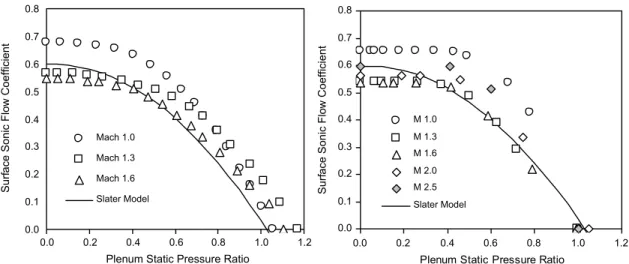
![Figure 5. Sonic flow coefficients for bleed flow through a single bleed hole [29].](https://thumb-us.123doks.com/thumbv2/123dok_us/1879031.2774280/65.918.260.715.405.693/figure-sonic-flow-coefficients-bleed-flow-single-bleed.webp)