Working paper n. 30 September/2010
On the use of Structural Equation Models
and PLS Path Modeling to build composite indicators
Laura Trinchera1 & Giorgio Russolillo2
1 University of Macerata, Dipartimento di Studi sullo Sviluppo Economico 2 University of Naples, Dipartimento di Matematica e Statistica
Laura Trinchera1 & Giorgio Russolillo2
1 University of Macerata, Dipartimento di Studi sullo Sviluppo Economico 2 University of Naples, Dipartimento di Matematica e Statistica
Sommario
Nowadays there is a pre-eminent need to measure very complex phenomena like poverty, progress, well-being, etc. As is well known, the main feature of a composite indicator is that it summarizes com-plex and multidimensional issues. Thanks to its features, Structural Equation Modeling seems to be a useful tool for building systems of composite indicators. Among the several methods that have been de-veloped to estimate Structural Equation Models we focus on the PLS Path Modeling approach (PLS-PM), because of the key role that esti-mation of the latent variables (i.e. the composite indicators) plays in the estimation process. In this work, first we present Structural Equation Models and PLS-PM. Then we provide a suite of statistical methodologies for handling categorical indicators in PLS-PM. In par-ticular, in order to take categorical indicators into account, we propose to use a modified version of the PLS-PM algorithm recently presented by Russolillo [2009]. This new approach provides a quantification of the categorical indicators in such a way that the weight of each quanti-fied indicator is coherent with the explicative ability of the correspon-ding categorical indicator. To conclude, an application involving data taken from a paper by Russet [1964] will be presented.
Keywords: Composite Indicators, Structural Equation Modeling, PLS Path Modeling, Categorical Indicators.
Corresponding author: Laura Trinchera ([email protected]). Department Informations:
Piazza Oberdan 3, 62100 Macerata - Italy Phone: +39 0733 258 3960 Fax: +39 0733 258 3970 e-mail: [email protected]
Nowadays there is a pre-eminent need to measure very complex phenomena like poverty, progress, wellbeing, etc. Since all these concepts are complex and latent concepts they can not be directly measured, several indicators are necessary to resume them. The challenges of constructing a global measure of wellbeing or of progress by using composite indicators is a much-discussed theme. In particular, in literature two aspects are investigate: i) the identi-fication of key indicators to be used; ii) the ways in which these indicators can be brought together to make a coherent system of information. How to choose these indicators is up to psychologists, sociologists and economists, while it’s up to statisticians to provide operational tools to aggregate these indicators in order to build composite indicators.
There is a fundamental division in the indicators literature between tho-se who chootho-se to aggregate variables into a composite indicators and thotho-se who do not, and prefer using a suite of indicators. There is no doubt that composite indicators are appealing, especially as an answer to the calls for a replacement of the single indicator approach or the use of a suite of indi-cators, as for example the Human Development Index (HDI) and the GDP to measure progress. As a matter of fact, using a unique measure obtained by combining indicators can indeed capture reality and can easily be used to garner media’s and policy makers’ attention. Moreover, the advantages of a composite indicator over a set of indicators include the creation of a bottom line. However, composite indicators have some disadvantages. First, the choice of the components of the composite indicator, like the choice of indicators in a suite of indicators approach, is subjective. Second, movemen-ts in composite indicators are difficult to interpret: when presented with an indicator moving in a certain direction, one often wants to know what com-ponents are driving the movement. And third, the weighting and aggregation process by which the variables are combined is regarded as arbitrary. There is, therefore, a danger that a composite index will oversimplify a complex sy-stem and give potentially misleading signals [Hall, 2005]. According to this, the selection of the weights and the way the indicators are combined do not seem to be a methodological but an empirical issue in many approaches to the aggregation of indices.
Here, we present a new approach to compute complex composite indica-tors where the computation of the weights as well the aggregation process are
not subjective. Both the steps are based on the statistical relations among indicators. In particular, Structural Equation Models (SEM) and specifical-ly PLS approach to SEM (PLS Path Modeling, PLS-PM), will be used to compute composite indicators.
According to Saisana et al. [2002], a composite indicator is a mathe-matical combination of single indicators that represent different dimensions of a concept whose description is the objective of the analysis. Thus, the main feature of a complex indicator is that it summarize complex and mul-tidimensional issues. In this optic, Mulmul-tidimensional Data Analysis (MDA) approach seems to be the most natural tool to compute composite indicators. In fact, in a MDA approach the computation of the weights is not subjective, but it is based on the statistical relations among elementary indicators. If all the indicators refer to a single latent concept, classical MDA techniques, like Factorial Analysis (FA) or Principal Component Analysis (PCA), can be used. These techniques allow us to assess the impact of each indicator on the composite indicator. However, often the several indicators used in the construction of a composite indicator express different aspects of a com-plex phenomenon, and so they can be conceptually split in several blocks of indicators. Each block can be resumed by a composite indicator, which is considered causative with respect to a second-order composite indicator. We will refer to this kind of index, which is a synthesis of composite indica-tors, as complex indicator. We can build complex indicators using Multiple Factorial Analysis (MFA) models. However, MFA assumes a causal relation only between composite indicators and the complex indicator. To make more flexible the system of composite indicators and in order to model causal rela-tions among them, Structural Equation Models (SEM) [Bollen, 1989; Kaplan, 2000] can be used. As a matter of fact, SEM models allow us to aggregate indicators taking into account both the indicators membership to blocks, and the causal relations among blocks. One of the most important advantages in using SEM is that it provides two kinds of weights: one measuring the impact of each indicator on the corresponding composite indicator, the other measuring the impact of the composite indicators on the complex indicator. This two levels of weights helps to understand which is the most important indicator in building composite indicators, as well which is the main driver in computing the complex indicator. In other words, using SEM models to build complex indicators leads to the construction of a system of weights and relations that allow us to understand the different aspects composing the
complex indicators.
Among the six criteria for the evaluation of Quality of Life Indexes pro-posed by the International Society for Quality of life Studies [Hagerty et al, 2001] we have the following:
• Have a clear and pratical purpose and that such purpose includes useful-ness for public policy and measurement of trends and levels of economic and social well-being;
• Be reported as a single number but capable of being broken down into components as a single number allows citizens and policy makers to assess whether overall quality of life is improving;
• The ability of the domain to be measured in both objective and subjec-tive dimensions. Both subjecsubjec-tive and objecsubjec-tive indicators are necessary, but not sufficient, conditions to capture the totality of life experience, so both should be included in quality of life measurement.
In Authors opinion, the use of SEM models to build composite and complex indicators meet these three issues. Indeed, SEM models allow us to compute complex indicators as single numbers capable of being broken down into com-ponents (composite indicators) also obtained as single numbers. Moreover, they allow us to take into account both objective and subjective dimensions. As a matter of fact, in a system of composite indicators, as the one obtained by using SEM models, it is possible to consider both indicators coming from official statistics and subjective measures.
Two different approaches exist to estimate model parameters in Structural Equation Models: the covariance-based techniques and thecomponent-based techniques. The first approach refers to the methods aiming at reproducing the sample covariance matrix of the observed (manifest) variables by means of the model parameters. In component-based techniques, instead, latent variable (i.e. both composite and complex indicators) estimation plays a main role. As a matter of fact, the aim of component-based methods is to provide an estimate of the latent variables in such a way that they are the most correlated with one another (according to the path diagram structure) and the most representative of each corresponding block of manifest variables. Among the several methods that have been developed to estimate Struc-tural Equation Models we focus on the component-based techinques, and in particular on PLS Path Modeling approach (PLS-PM) [Wold, 1975; Tenen-hau et al., 2005], because the estimation of the latent variables plays a key
Furthermore, since categorical variables could be used as simple indicators in defining complex composite indicators, the role and the treatment of this kinds of variables in PLS-PM will be discussed in details (cf. section 3). To conclude, an application involving data taken from a paper by Russet [1964] will be presented.
2 Structural Equation Modeling and PLS Path Modeling 2.1 Introduction to Structural Equation Models
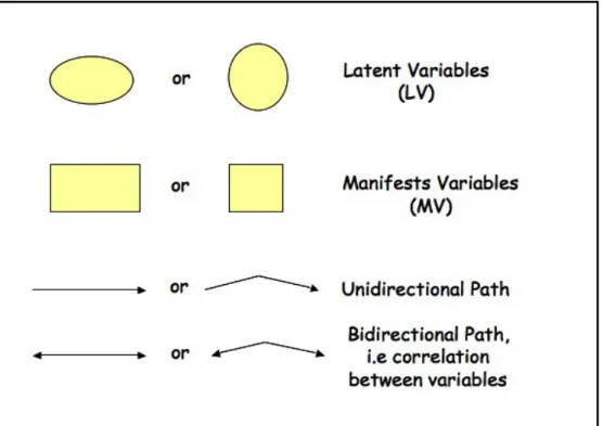
SEM models include a number of statistical methodologies that allow us to estimate the causal relationships, defined according to a theoretical model, linking two or more latent complex concepts (i.e. the composite indicators), each measured through a number of observable indicators. The basic idea is that complexity inside a system can be studied taking into account a whole of causal relationships among latent concepts, called Latent Variables (LV), each measured by several observed indicators usually defined as Manifest Va-riables (MV). It is in this sense that, Structural Equation Models represent a joint-point between the path analysis and the Confirmatory Factor Analysis. Factor Analysis presumes that a number of factors (i.e. the latent variables) smaller than the number of observed variables are responsible for the shared variance-covariance among the observed variables. Hence, SEM receive from Confirmatory Factor Analysis the idea that different subsets or blocks of va-riables are expression of different concepts. Moreover, path models are a logical extension of regression models as they involve the analysis of simul-taneous multiple regression equations. More specifically, a path model is a relational model with direct and indirect effects among observed variables, while multiple-multivariate regression models being additive by definition, only take into account direct relationships between the independent varia-bles and the dependent variavaria-bles. When the variavaria-bles inside the path model are latent variables whose measure is inferred by a set of observed indicators path analysis is termed Structural Equation Modeling. The conceptual model behind the relations among latent and manifest variables is drawn as aPath diagram in which ellipses or circles represent the latent variables and
rectan-Figura 1: Commonly used symbols in Structural Equation Models
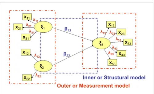
gles or squares refer to the manifest variables (see figure 1). Arrows show causations among the variables (either latent or manifest), and the direction of the array defines the direction of the relation, i.e. variables receiving the array are to be considered as endogenous variables in the specific relationship (see figure 2). Each SEM model involves two levels of relationships: the first one takes into account the relations between the MVs and the corresponding LV (measurement model), the latter considers the causal relations among the LVs (structural model). Thus, the endogenous LVs can be seen not only as composite indicators, due to their relations with the corresponding indica-tors, but also as complex indicaindica-tors, due to their causal relations with other composite indicators.
Several methods have been developed to estimate both measurement and structural model parameters, among them the PLS Path Modeling approach (PLS-PM) [Wold, 1975 and 1982]. PLS-PM is a so-called component-based
Figura 2: Structural Equation Model representation
estimation method, because of the key role that is played by the estimation of the LVs in the model. The main aim ofcomponent-based methods, in fact, is to provide an estimateˆξ of each LV (ξ) in such a way that they are the most correlated with one another (according to the path diagram structure) and the most representative of each corresponding block of manifest variables. This is of main importance in building system of composite indicators. As a matter of fact, according to PLS-PM approach, each composite indicator is obtained in order to be the most representative of each corresponding indicator and the most correlated with the others linked composite indicators. In the following, first an historical review of Structural Equation Models is furnished (see sub-section 2.1.1), then a brief review of the PLS-PM algorithm is provided (see sub-section 2.2). For a complete review of the PLS approach to SEM please refers to Tenenhaus et al. [2005].
2.1.1 Structural Equation Model: an historical review
Essentially developed in a social domain, Structural Equation Models were first introduced by Jöreskog [1970] as confirmatory models to assess cause-effect relations among two or more set of variables, based on the maximum likelihood (ML) estimation method (SEM-ML). This method, also known as LISREL (LInear Structural RELations), has been for many years the only estimation method for SEM. The term LISREL was initially used for the soft-ware implementing the methodology Jöreskog and Sörbon [1996]. However, it had such a rapid development that the methodology and the software have been associated to each other. Furthermore, it is important to notice that other estimation techniques rather than the maximum likelihood approach can be used to estimate Structural Equation Models, such as the Genera-lized Least Squares (GLS) or the Asymptotically distribution free (ADF). All these methods are usually referred to as LISREL-type estimation tech-niques. The common factor to all the LISREL-type estimation techniques is that they are the so-called covariance-based methods. As a matter of fact, all these techniques aim at reproducing the sample covariance matrix of the manifest variables by means of the model parameters. The fundamental hy-pothesis underlining these approaches is that the implied covariance matrix of the manifest variables is a function of the model parameters.
In 1975, Wold [1975] finalized asoft modelingapproach to the analysis of the relations among several blocks of variables observed on the same stati-stical units. This method, known as PLS approach to SEM (SEM-PLS) or as PLS Path Modeling (PLS-PM), is a distribution-free approach that was developed as a flexible technique for handling a huge amount of data charac-terized by missing values, strongly correlated variables and a small sample size as compared to the number of variables.
Several authors have compared the two approaches over the years; see, for example, Jöreskog and Wold [1982], Fornell and Bookstain [1982], Djk-stra [1983]. The two approaches differ in the objectives of the analysis, the statistical assumptions, the estimation procedures and the related outputs.
New estimation techniques for Structural Equation Model have been pre-sented recently. Namely, in 2003 Al-Nasser proposed to extend Information theory knowledge at Structural Equation Models context via a new technique called Generalized Maximum Entropy (GME) [Al-Nasser, 2003].
Structured Component Analysis (GSCA). These new estimation techniques remain in the optic of PLS approach to SEM since no distributional assump-tions are required. Moreover, the same problems characterizing the PLS-PM, namely the lack of a global optimizing criterion, have yet to be successfully solved.
PLS-PM, GME, and GSCA approaches to Structural Equation Models have to be considered ascomponent-basedestimation techniques. As a matter of fact, in all these techniques the latent variable estimation plays a central role. In the next sub-section a deep presentation of PLS approach to SEM will be provided.
2.2 PLS approach to Structural Equation Models
As already said, the aim ofcomponent-basedmethods is to provide an estima-te of the laestima-tent variables in such a way that they are the most correlaestima-ted with one another (according to the path diagram structure) and the most repre-sentative of each corresponding block of manifest variables. These techniques are to be considered as a generalization of Principal Component Analysis to multi-tables data linked to one another. Here we focus on the PLS (Partial Least Squares) approach to Structural Equation Models, also known as PLS Path Modeling (PLS-PM) [Wold, 1975; Tenenhaus et al., 2005].
PLS-PM has been proposed as an alternative estimation procedure to the LISREL-type approach to Structural Equation Models. In Wold’s seminal paper [Wold, 1975] the main principles of partial least squaresfor the princi-pal component analysis [Wold, 1966], were extended to situations with more blocks of variables. The first presentation of the PLS Path Modeling is given in Wold [1979], and the algorithm is described in Wold [1982] and in Wold [1985]. An extensive review on PLS approach to Structural Equation Models is given in Chin [1998] and in Tenenhaus et al. [2005].
PLS Path Modeling is an iterative algorithm that separately estimates the several blocks of the measurement model and then, in a second step, estimates the structural model coefficients. Differently from LISREL-type estimation techniques, PLS Path Modeling aims at explaining at best the residual variance of the latent variables and, potentially, also of the manifest variables in any regression run in the model [Fornell and Bookstain, 1982]. That is why PLS Path Modeling is considered more an explorative approach than a confermative one: it does not aim at reproducing the sample
covarian-ce matrix. Moreover, differently from LISREL-type estimation techniques, the PLS Path Modeling is a completely free approach that does not require any distributional assumption. For this reason the PLS-PM is considered as a soft modelingapproach: no strong assumptions (with respect to the di-stributions, the sample size and the measurement scale) have to be made. Nevertheless, PLS-PM does not seem to optimize a well identified global sca-lar function. Until now convergence is proved only for path diagram with one or two blocks [Lyttkens et al., 1975]. Researches on this topic are on going. Further, PLS Path Modeling provides a direct estimate of the latent variable scores.
2.2.1 The PLS Path Modeling Algorithm
PLS Path Modeling aims to estimate the relationships among Q blocks of variables, which are expression of unobservable constructs. Specifically, PLS-PM estimates through a system of interdependent equations based on simple and multiple regressions, the network of relations among the manifest varia-bles and their own latent variavaria-bles, and among the latent variavaria-bles inside the model.
Formally, let us assume P variables observed on N units (i = 1, . . . , N). The resulting data xnpq are collected in a partitioned table of standardized data X:
X = [X1, . . . ,Xq, . . . ,XQ], where Xq is the genericq-th block.
Each SEM model involves two levels of relationships: the first one (the mea-surement model) takes into account the relations between the MVs and the corresponding LV (ξq), the latter considers the causal relations among the LVs (structural model). In PLS-PM for each endogenous LV in the model, the structural model can be rewritten as:
ξj =β0j+
X
q:ξq→ξj
βqjξq+ζj (1)
where ξj (j = 1, . . . , J) is the generic endogenous latent variable, βqj is the generic path coefficient interrelating the q-th exogenous latent variable to the j-th endogenous one, and ζj is the error in the inner relation (i.e. disturbance term in the prediction of the j-th endogenous latent variable
from its explanatory latent variables). The measurement model formulation depends on the nature of the relationships between the latent variables and the corresponding manifest variables. As a matter of fact, different types of measurement models are available: the formative model, thereflective model and the MIMIC model.
In a reflective model the block of manifest variables related to a latent variable is assumed to measure a unique underlying concept. Each manifest variable reflects (is an effect of) the corresponding latent variable and plays a role of endogenous variable in the block specific measurement model. In the reflective measurement model, indicators linked to the same latent va-riable should covary: changes in one indicator imply changes in the others. Moreover, internal consistency has to be checked, i.e. each block is assumed to be homogeneous and unidimensional. It is important to notice that for the reflective models, the measurement model reproduces the factor analysis model, in which each variable is a function of the underlying factor. In more formal terms, in a reflective model each manifest variable is related to the corresponding latent variable by a simple regression model, i.e:
xpq =λp0+λpqξq+pq (2) where λpq is the loading associated to the p-th manifest variable in theq-th block and the error term pq represents the imprecision in the measurement process. An assumption behind this model is that the error εpq has a zero mean and is uncorrelated with the latent variable of the same block:
E(xpq|ξq) = λp0+λpqξq. (3)
This assumption, defined as predictor specification, assures desirable estima-tion properties in classical Ordinary Least Squares (OLS) modeling.
In the formative model , each manifest variable or each sub-block of ma-nifest variables represents a different dimension of the underlying concept. Therefore, unlike the reflective model, the formative model does not assume homogeneity nor unidimensionality of the block. The latent variable is de-fined as a linear combination of the corresponding manifest variables, thus each manifest variable is an exogenous variable in the measurement model. These indicators need not to covary: changes in one indicator do not imply changes in the others and internal consistency is no more an issue. Thus the
measurement model can be expressed as: ξq = Pq X p=1 ωpqxpq +δq (4)
whereωpqis the coefficient linking each manifest variable to the corresponding latent variable and the error termδq represents the fraction of the correspon-ding latent variable not accounted for by the block of manifest variables. The assumption behind this model is the following predictor specification:
E(ξq|xpq) = Pq
X
p=1
ωpqxpq. (5)
Finally, the MIMIC model is a mixture of both the reflective and the formative models within the same block of manifest variables.
Independently from the type of measurement model, upon convergence of the algorithm, the standardized latent variable scores (ξˆq) associated to the q-th latent variable (ξq) are computed as a linear combination of its own block of manifest variables by means of the so-calledweight relations defined as: ˆ ξq= Pq X p=1 wpqxpq (6)
where the variables xpq are centred and wpq are the outer weights. These weights are yielded upon convergence of the algorithm and then transformed so as to produce standardized latent variable scores. However, when all manifest variables are observed on the same measurement scale and all outer weights are positive, it is interesting and feasible to express these scores in the original scale [Fornell, 1992]. This is achieved by using normalized weights
˜ wpq defined as: ˜ wpq = wpq PPq p=1wpq with Pq X p=1 ˜ wpq = 1 ∀q :Pq >1. (7)
In PLS Path Modeling an iterative procedure allows us to estimate the model parameters, i.e the outer weights (wpq) and the latent variable scores (ξq). The estimation procedure is namedpartialsince it solves blocks one at a time by means of alternating single and multiple linear regressions. The
path coefficients (βqj) come afterwards from a regular regression between the estimated latent variable scores.
The estimation of the latent variable scores are obtained through the alter-nation of the outerand theinnerestimations, iterating till convergence. The procedure works on centred (or standardized) data and starts by choosing arbitrary weights wpq. Then, in the external estimation, each latent variable is estimated as a linear combination of its own manifest variables:
νq ∝ ± Pq
X
p=1
wpqxpq =Xqwq (8)
where νq is the standardized outer estimation of the q-th latent variable ξq, the symbol ∝ means that the left side of the equation corresponds to the standardized right side and the ± sign shows the sign ambiguity. This ambiguity is usually solved by choosing the sign making the outer estimate positively correlated to a majority of its manifest variables. Anyhow, the user is allowed to invert the signs of the weights for a whole block in order to make them coherent with the definition of the latent variable.
In the internal estimation, each latent variable is estimated by considering its links with the other Q0 adjacent latent variables:
ϑq ∝ Q0
X
q0=1
eqq0νq (9)
where ϑq is the standardized inner estimation of the q-th latent variable ξq and the inner weights (eqq0) are equal (in a centroid scheme) to the signs of the correlations between the q-th latent variable νq and the νq0s connected with νq. Inner weights can be obtained following other schemes rather than the centroid one. Namely, the inner weights can be equal to:
1. the signs of the correlations between the q-th latent variable νq and the νq0s connected with νq in the centroid scheme (the Wold’s original scheme)
2. the correlations between the q-th latent variable νq and the νq0s con-nected with νq in the factorial scheme (the Löhmoller scheme)
3. the multiple regression coefficient ofνq and the νq0s connected withνq, if the νq is the inner estimation of an endogenous latent variables, or the correlations coefficient for exogenous latent variables in structural scheme.
Once a first estimation of the latent variables is obtained, the algorithm goes on by updating the outer weights wpq.
Two different ways are available to update the outer weights usually related to the two different kinds of measurement model (i.e. the formative or the reflective scheme):
• Mode A: each outer weight wpq is the regression coefficient in the simple regression of the p-th manifest variable of the q-th block (xpq) on the inner estimate of the q-th latent variable ϑq. As a matter of fact, since the latent variable score xpq is standardized, the generic outer weight
wpq is obtained as:
wpq =cov(xpq,ϑq) (10)
i.e. as the covariance between each manifest variable and the correspon-ding inner estimate of the latent variable.
• Mode B: the vector wq of the weights wpq associated to the manifest variables of the q-th block is the regression coefficient vector in the multiple regression of the inner estimate of the q-th latent variable ϑq on its centered manifest variables Xq:
wq = X0qXq
−1
X0qϑq (11)
As already said, the choice of the external weight estimation mode is strictly related to the nature of the model. For areflective modeltheMode Ais more appropriate, while Mode B is better for the formative model. Furthermore, Mode A is suggested for endogenous latent variables, while Mode B for the exogenous ones. It is worth noticing thatMode Bis affected by multicollinea-rity. In such a situation, PLS regression may be used as a valuable alternative to OLS regression to obtain the external weights according to equation 11 [Esposito Vinzi et al., 2010].
The algorithm is iterated till convergence, which is demonstrated to be reached for one and two-block models. However, for multi-block models, convergence is always verified in practice. After convergence, structural (or path) coefficients are estimated through an OLS multiple regression among the estimated latent variable scores.
Wold’s original algorithm has been further developed [Löhmoller, 1987; 1989]. In particular, new options for computing both inner and outer estima-tions have been implemented together with a specific treatment for missing
data and multicollinearity [Tenenhaus et al., 2005a]. As regards this last point, in the case of multicollinearity among the estimated latent variables, PLS regression can be used to obtain path coefficient estimates instead of OLS regression [Esposito Vinzi et al., 2010].
2.2.2 The Quality indexes
PLS Path Modeling lacks a well identified global optimization criterion so that there is noglobal fitting functionto be evaluated to determine the good-ness of the model. Furthermore, it is a variance-based model strongly orien-ted to prediction. Thus, model validation focuses on the model predictive capability. According to PLS-PM structure, each part of the model needs to be validated: the measurement model, the structural model and the overall model. That is why, PLS Path Modeling provides three different fit indexes: thecommunalityindex, theredundancyindex and theGoodness of Fit(GoF) index.
For each q-th block in the model with more than one manifest variable (i.e. for each block with Pq > 1) the quality of the measurement model is assessed by means of the communality index:
Comq = 1 Pq Pq X p=1 cor2 xpq,ξˆq ∀q :Pq >1. (12)
This index measures how much of the manifest variable variability in theq-th block is explained by its own latent variable ξq. That means how well the manifest variables describe the related latent variable. Moreover, the com-munality index for the q-th block is nothing but the average of the squared correlations between each manifest variable in the q-th block and the q-th latent variable.
It is possible to measure the quality of the whole measurement model by means of the average communality index, i.e:
Com= P 1
q:Pq>1Pq
X
q:Pq>1
PqComq. (13)
This is a weighted average of all the Q block-specific communality indexes (see equation 12) with weights equal to the number of manifest variables in each block. Moreover, since the communality index for the q-th block is nothing but the average of the squared correlation in the block, then the
average communality is the average of all the squared correlations between each manifest variable and the corresponding latent variable in the model, i.e.: Com= P 1 q:Pq>1Pq X q:Pq>1 Pq X p=1 cor2xpq,ˆξq . (14)
Although the quality of each structural equation is measured by a sim-ple evaluation of the classical R2 fit index, this is not sufficient to evaluate the whole structural model. Specifically, since the structural equations are estimated once the convergence is assured, i.e. once the latent variable sco-res are estimated, then the R2 values only take into account the fit of each
regression in the structural model. That is why a new index is computed for each endogenous block in addition to the R2 value in order to take into account also the measurement model: the redundancy index.
The redundancy index computed for the j-th block, measures the portion of variability of the manifest variables connected to the j-th endogenous latent variable explained by the latent variables directly connected to the block, i.e.: Redj =Comj×R2 ˆ ξj,{ˆξq:ξ q→ξj (15) A global quality measure of the structural model is also provided by the average redundancy index, computed as:
Red= 1 J J X j=1 Redj (16)
where J is the total number of endogenous latent variables in the model. As aforementioned, there is no overall fit index in PLS Path Modeling. Nevertheless, a global criterion of goodness of fit has been recently proposed by Amato et al. [2005]: the GoF index. Such index has been developed in order to take into account the model performance in both the measurement and the structural model. For this reason the GoF index is obtained as the geometric mean of theaverage communalityindex and the average R2 value:
GoF =pCom×R2 (17)
where the average R2 value is obtained as: R2 = 1 JR 2ˆξ j,ξˆq:ξq→ξj . (18)
As it is partly based on average communality, theGoF index is conceptually appropriate whenever measurement models are reflective. However, commu-nalities may be also computed and interpreted in case of formative models knowing that, in such a case, we expect lower communalities but higher R2
as compared to reflective models. Therefore, for practical purposes, theGoF
index can be interpreted also with formative models as it still provides a measure of overall fit. According to equations (14) and (18) the GoF index can be rewritten as:
GoF = v u u t P q:Pq>1 PPq p=1Cor2 xpq,ˆξq P q:Pq>1Pq × PJ j=1R2 ˆ ξj,ξˆq:ξ q→ξj J . (19) As PLS Path Modeling is a soft modeling approach with no distributional assumptions, it is possible to estimate the significance of the parameters based on cross-validation methods like jack-knife and bootstrap [Efron and Tibshirani, 1993]. It is also possible to build a cross-validated version of all the quality indexes (i.e. of the communality index, of the redundancy index, and of theGoF index) by means of ablindfoldingprocedure. For more details on the blindfolding procedure please refers to Tenenhauset al. [2005].
A normalized version of the GoF has been presented by Tenenhaus et al. [2004]. This index is obtained by relating each term in equation 19 to the corresponding maximum value. In particular, it is well known that in principal component analysis the best rank one approximation of a set of variables X is given by the eigenvector associated to the largest eigenvalue
λ of the XTX matrix. Furthermore, the sum of the squared correlation between each variable and the first principal component ofX is a maximum. Therefore, if data are mean centered and with unit variance, the first term in equation 19 is such that PPq
p=1cor 2x
pq,ˆξq
≤ λ1
q, where λ1(q) is the first
eigenvalue obtained by performing a Principal Component Analysis on the
q-th block of manifest variables. Thus, the normalized version of the first term of the GoF is obtained as:
T1 = 1 P q:Pq>1Pq X q:Pq>1 PPq p=1cor 2x pq,ξˆq λ1 (q) . (20)
In other words, here the sum of the communalities in each block is divided by the first eigenvalue of the block.
T2 = 1 J J X j=1 R2ξˆ j,ξˆq:ξq→ξj ρ2 j (21)
where ρj is the first canonical correlation of the canonical analysis of matri-ces Xj containing the manifest variables associated to the j-th endogenous latent variable, and Xq containing the manifest variables associated to the exogenous latent variables explaining ξq.
Thus, according to equations 20, 21 and 19, the relative GoF index is:
GoFrel= v u u u t 1 P q:Pq>1Pq X q:Pq>1 PPq p=1Cor2 xpq,ξˆq λ1 (q) × 1 J J X j=1 R2ˆξ j,ˆξq:ξq→ξj ρ2 j (22) This index, is bounded between 0 and 1. Both the GoF and the relative
GoF are descriptive indexes, i.e. there is no inference-based threshold to judge their values. Nonetheless, the higher their value is, the best the model performance is. As a rule of thumb, a value of the relative GoF equal to or higher than 0.9clearly speaks in favor of the model.
3 The role of categorical variables in a PLS-PM model
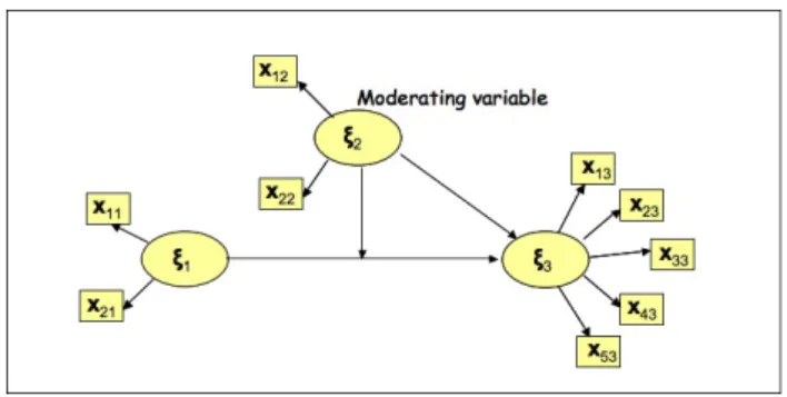
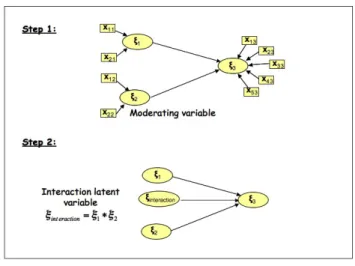
PLS-PM is a technique born to handle quantitative variables. However, in the practice categorical indicators could be used to measure complex concep-ts as well. In particular, a categorical variable can play two different roles in a PLS-PM: an active role and a moderating role. An active categori-cal variable directly participates in the construction of the model. In other words, an active categorical variable is a categorical indicator impacting on a composite indicator jointly with other quantitative indicators. A moderating categorical variable, instead, is a variable that does not play a direct role in the construction of the composite indicators. This variable influence the re-lationships, in terms of strength and/or direction, between an exogenous and an endogenous variables [Baronet al., 1986] (see fig. 3). The so called mode-rating effectcan be seen as the effect obtained by considering several groups of units each defined by a category of the categorical moderating variable.
Figura 3: Moderating Variable in a simple SEM
In this section we investigate both the use of categorical variables as in-dicators and as moderating variables. First, we investigate the case of mo-derating categorical variable (cf. sub-section 3.1). Then, a modified version of the PLS-PM algorithm able to handle both categorical and quantitative indicators will be presented (cf. sub-section3.2).
3.1 Using categorical variables as moderating variables PLS-PM model
Different approaches have been proposed in literature to model moderating categorical variables. In particular, we propose to distinguish between mani-fest moderating categorical variables and latent moderating categorical va-riables. Manifest moderating categorical variables are usually modeled by adding a so-called interaction term as an additional LV in the model [Kenny et al., 1984]. A latent moderating categorical variable, instead, is usually considered as a LV defining latent classes.
3.1.1 Manifest moderating categorical variables
As already said, categorical moderating variables are variables influencing the relationship, in terms of strength and/or direction, between an endo-genous and an exoendo-genous variable [Baron et al., 1986]. The effects of this variables can be seen as the effect obtained by considering several groups of units each defined by a category of the manifest moderating categorical
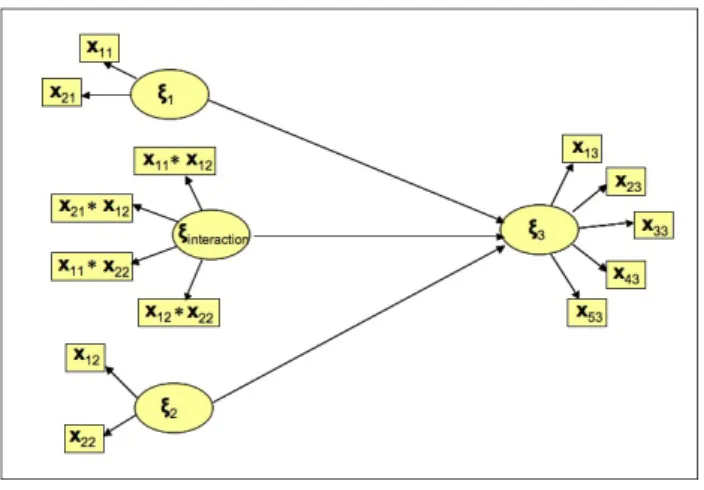
variable. In classical SEM moderating variables have been integrated by ad-ding a so-called interaction term as an additional LV in the model [Kenny et al., 1984]. In a simple model, with only one exogenous variable and one endogenous variable, the interaction term is obtained as the product of the indicators linked to the exogenous latent variable and the moderating va-riable (see fig. 4). In such a model, it does not matter which vava-riable is moderating and which one is the exogenous one. Moreover, problems arise in the interpretation of the product term.
Figura 4: Creating interaction term in a simple SEM by product
A first attempt to take into account moderating variables in PLS-PM by including interaction effects was made by Chin et al. [2003]. Since then, other proposals exist for modeling moderating effects in PLS-PM framework, as the one by Henseler et al. [2010], and the one by Tenenhauset al. [2010]. In particular, Henseler et al. [2010] propose to use a two step procedure to include product terms. In the first step they suggest performing PLS-PM by considering both the exogenous variable and the moderating variable as independent LVs in the model. Once LV scores are estimated, the product term is computed as the elementwise product of the exogenous LV scores and the moderating LV score. A multiple linear regression between the endoge-nous LV scores, the moderating LV scores, and the product term LV scores
is then performed. A scheme of procedure proposed by Henseleret al. [2010] is shown in figure 5.
Figura 5: Henseler and Fassot procedure to model interaction effect in a simple SEM with formative indicators
Chin et al. [2003] suggest to assess the moderating effect by comparing the R2 values, i.e. the proportion of the variance explained by the model, computed for the model without moderating effect with theR2value obtained
for the model taking into account interaction effects. The effect size, f2, is
computed as:
f2 = R 2
model with moderating−R2model without moderating 1−R2
model without moderating
(23) Moderating effects with an effect size f2 of 0.02 are regarded as weak, an effect size between 0.15and 0.35as moderated and an effect size higher than 0.35 as strong [Chin et al., 2003]. Nevertheless, the authors stress that a lower effect size does not necessarily mean that the considered moderating effect is negligible. The significance of the coefficient linked to the interaction effect can be tested also by means of bootstrap-based techniques [Henseler et al., 2010].
Manifest moderating categorical variables playing the role of class-membership variable are very common in practice. Also in composite indicators
fra-meworks is of main importance to take into account manifest moderating categorical variables when computing composite indicators. For instance, gender-specific indexes, as the GDI (Gender-related Development Index) of the United Nations Development Program, involve taking into account the same variables for female and male. In other words, the gender variable play the role of a manifest moderating categorical variable.
3.1.2 Latent moderating categorical variables
If no manifest moderating variables are available, several clustering techni-ques have been developed in SEM and in PLS-PM to look for latent classes. Among them, some techniques allow obtaining latent classes by taking in-to account the causal structure of the model: the so-called response-based clustering techniques [Trinchera, 2007]. When information concerning the causal relationships among variables is available (as it is in the theoretical causal network of relationships defining a SEM model), classes should be looked for while taking into account this relevant piece of information. That is why response-based methods have to be preferred to classical clustering techniques, such as cluster analysis. As a matter of fact, in response-based clustering methods, the obtained classes are homogeneous with respect to the postulated model, i.e. with respect to the weights used to compute com-posite and complex indicators. This approach to clustering is opposed to the traditional a priori clustering, where classes are defined according to infor-mation which is not related to the existing model but depends on external criteria.
Response-based clustering techniques allow us to obtain local models, i.e. class-specific models. Each local model is characterized by class-specific para-meters. In other words, these methods assume that in the observed data-set several groups of units exist, each characterized by different models. To the authors’ knowledge, two main methods exist to obtain response-based clu-sters in PLS-PM: the Finite Mixture PLS, proposed by Hahn et al. [2002] and modified by Ringle et al. [2010], and the REsponse Based Unit Segmen-tation in PLS Path Model (REBUS-PLS) [Trinchera, 2007; Esposito Vinzi et al., 2008].
FIMIX-PLS is an extension of Finite Mixture Models [McLachlan et al., 2000] to the case of PLS-PM. The basic idea is that statistical units come from a mixture of normal populations, and the aim is to find a probability
that each unit belongs to each class. A central role in FIMIX-PLS is played by the LV scores, used in an EM (Expectation-Maximization) procedure to obtain a fuzzy classification of units. Nevertheless, the EM procedure requi-res the normal distribution at least for the predicted LVs. This is not in line with PLS-PM features that is a distribution-free technique. Moreover, the obtained local models will be different only with respect to the structural models, the LV scores are considered as fixed, at least in the original formu-lation of the algorithm [Hahn et al., 2002]. Ringle et al. [2010] propose to solve this problem by looking for an external variable able to obtain similar classes as those identified by FIMIX-PLS, and to perform PLS-PM on ea-ch of those classes. As a result, the obtained local models will be different both for the structural and the measurement models, nevertheless it is not easy to obtain similar classes by using available external variables. The last drawback of FIMIX-PLS is that the number of classes is not considered as a parameter to be estimated, and have to be decide a priori.
In order to overcome the main limits of the FIMIX-PLS a new method for latent classes detection in PLS-PM has been recently developed: the REBUS-PLS [Trinchera, 2007; Esposito Vinzi et al., 2008]. Unlike FIMIX-PLS and according to PLS-PM features, REBUS-PLS does not require distributional hypotheses. Moreover, REBUS-PLS has been developed so as to detect he-terogeneity both in the structural and the measurement models. The idea is that if latent classes exist, units belonging to the same latent class will have similar local models, i.e. similar performance as regard to the global model. Moreover, if a unit is correctly assigned to a latent class, its performance in the local models computed for that class will be better than the performance obtained by the same unit in all the other local models. For these reasons the units are assigned to the latent classes according to a “closeness measu-re” (CM) taking into account the residuals of each unit with respect to each local model. The chosen CM is defined in order to obtain local models that are better fitted than the global model for both the measurement and the structural models. A description of the REBUS-PLS algorithm is given in algorithm 2. For more details please refer to Esposito Vinzi et al. [2008]. Until now, REBUS-PLS has only been developed for models showing a re-flective measurement model. Development of the REBUS-PLS algorithm to take into account also formative indicators are on going.
Algorithm 1 REBUS-PLS algorithm
Step 1: Estimation of the global PLS Path Model
Step 2: Computation of the communality and structural residuals of all unit from the global model
Step 3: Hierarchical classification on the residuals computed at step 2 Step 4: Choice of the number of classes (K) according to the dendrogramme obtained at step 3
Step 5: Assignment of the units to each class according to the cluster analysis results
repeat
for all k = 1, . . . , K do
Step 6: Estimation of the k-th local model
Step 7: Computation of the closeness measure of each unit from the k-th local model
end for
Step 8: Assignment of each unit to the closest local model until stability in class membership
Step 9: Computation of the final K local models according to class membership obtained by the iterative procedure
3.2 Using quantitative indicators as manifest variables in a PLS-PM model
Until now, composite indicators are obtained only as a mathematical combi-nation of single (quantitative) indicators [Saisana et al., 2002]. However, to take into account also categorical indicators in building composite indicators is very fascinating. For instance, when computing complex and composite indicators, it could be interesting take into account demographical variables, such as religion or gender, and/or categorical variables defining states, such as government form.
The most common approach for introducing categorical indicators as MVs in a PLS-PM is their replacement with the corresponding dummy matrix
˜
Xpq. Each element x˜il of X˜pq is equal to one if the i-th observation shows the l-th modality, otherwise is zero. However, this approach have an impor-tant drawback: it measures the impact of each modality on the composite indicator. As a consequence, the global influence of a categorical indica-tor is not directly measured. Moreover, the indirect weight of a categorical indicator in the construction of a LV increases as well as the number of the modalities increases. To overcome these drawbacks, quantification-based techniques have been recently proposed in literature. These algorithms as-sign a numeric value to each category in order to get quantified indicators that can be handled as they were quantitative.
Partial Maximum Likelihood (PML) algorithm [Jakobowiczet al., 2007] is an adapted version of PLS-PM aimed to generalize PLS approach when the indicators are of different nature. PLM’s authors advise to estimate weights of nominal and boolean indicators by PLM because it seems to significantly improve the quality of the model when a number of indicators have this nature. However, PLM provides the impacts of each category, while the global impact of each categorical indicator is not provided by the algorithm but it is indirectly calculated a posteriori. Furthermore, it is not specified how these impacts can be interpreted. As matter of fact, PML algorithm can be seen as an optimal scaling procedure, without a well specified optimality criterion.
Here, we present a modification of the PLS-PM as recently proposed by Russolillo [2009]: the Non-Metric PLS-PM (NM-PLSPM). This approach makes it possible to handle categorical variables as they were measured on a interval scale. The aim is to provide an optimally scaling of the
catego-categories. This quantification criterion assures that the role of the quanti-fied indicators is coherent with the explicative ability of the corresponding categorical indicator. In order to get quantifications with such properties, a modified PLS-PM algorithm that estimates at the same time both the model parameters and the scaling parameters of the categorical indicators has been recently presented by Russolillo [2009].
In the Non-Metric PLS-PM algorithm the computation of the LVs starts with an arbitrary choice of their inner estimates ϑ1, . . . ,ϑQ. Afterwards, a new first step is added in each cycle of the iterative procedure. It is a quantification step, in which each categorical indicator is transformed in a quantitative one; this new quantified indicator x∗pq is obtained as the ortho-gonal projection of ϑq on the space spanned by the columns ofX˜pq. From a computational point of view,
x∗pq = ˜Xpq ˜ X0pqX˜pq −1 ˜ X0pqϑq (24)
The procedure continues with the second and the third steps, i.e. the inner estimation and the outer estimations of each LV according to equations 9 and 8. Once new outer estimates are computed, the cycle restarts with the quantification step and it is iterated until the convergence between inner and outer estimations is reached.
This procedure yields as output both scaling and model parameters. It assures that quantified indicators show suitable properties in terms of op-timality and interpretability. The scaling parameters maximize correlation of the quantified indicator with the inner estimate of the own LV, and as consequence its weight in the construction of the LV in a reflective scheme. Moreover, the weight of each quantified indicator can be expressed also in terms of part of variability of ϑq explained byxpq˜ ’s modalities. In particular, it is possible to show the following equivalence:
ρx∗
pq,ϑq =ηxpq,ϑq (25) Hence, the weight of x∗pq reflects the predictive capability of the categories of xpq with respect to ϑq, measured by the correlation ratio squared root. It is for this reason that the NM-PLSPM algorithm is very useful to yield reliable weights for building composite and complex indicators from simple indicators observed on a variety of measurement scales.
4 An application to macroeconomic data: the Russet data
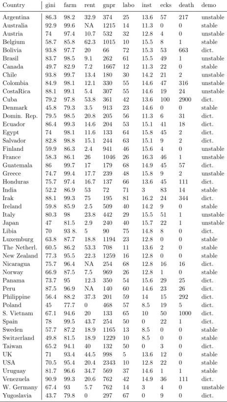
The data for this example (see table 1) are taken from a paper by Russet [1964]. The basic hypothesis in Russet’s paper is that economic inequali-ty leads to political instabiliinequali-ty. In particular in the Russet model political instability is a function of inequality of land distribution and of industrial development. Three indicators are used to measure inequality of land distri-bution. Indicator gini is Gini’s index of concentration, which measures the deviation of the Lorenz curve from the line of equality. The indicator farm is the percentage of farmers that own half of the lands, starting with the smallest ones. Thus if farm is 90%, then 10% of the farmers own half of the land. The third indicator is rent, which is the percentage of farm households that rent all their land. Two indicators are used to measure industrial de-velopment: indicator gnpr is the gross national product pro capite (in U.S. dollars) in 1955, and the indicator labo is the percentage of labor force em-ployed in agriculture. Political stability is measured by four indicators. The indicator inst is a function of the number of the chiefs of the executive and of the number of years of independence of the country during the period 1946-1961. This index bounds between 0 (very stable) and 17 (very unsta-ble). The indicator ecks is Eckstein’s index, which measures the number of violent internal war incidents during the same period. The indicatordeathis the number of people killed as a result of violent manifestations during the period 1950-1962. The indicator demo classifies countries in three groups: stable democracy, unstable democracy and dictatorship.
This data-set was analyzed in Gifi [1990] using the program CANALS (Canonical Correlation Analysis by Alternating Least Squares). Variables were scaled in such a way as to maximize the canonical correlation between the block of variables regarding the economic inequality and the block of variables regarding the political instability. However, Gifi himself noticed that partitioning data in the three sets of variables (agricultural inequality, industrial development and political instability) would have been a more rational approach.
Starting from this idea, Tenenhaus [1998] modeled the Russet data-set in a PLS-PM framework (see figure 6). He partitioned the Russet data-set in three reflective blocks. The first block, consisting of the manifest variables gini, farmand rentmeasures the latent variable, i.e. the composite
Country gini farm rent gnpr labo inst ecks death demo Argentina 86.3 98.2 32.9 374 25 13.6 57 217 unstable Australia 92.9 99.6 NA 1215 14 11.3 0 0 stable Austria 74 97.4 10.7 532 32 12.8 4 0 unstable Belgium 58.7 85.8 62.3 1015 10 15.5 8 1 stable Bolivia 93.8 97.7 20 66 72 15.3 53 663 dict. Brasil 83.7 98.5 9.1 262 61 15.5 49 1 unstable Canada 49.7 82.9 7.2 1667 12 11.3 22 0 stable Chile 93.8 99.7 13.4 180 30 14.2 21 2 unstable Colombia 84.9 98.1 12.1 330 55 14.6 47 316 unstable CostaRica 88.1 99.1 5.4 307 55 14.6 19 24 unstable Cuba 79.2 97.8 53.8 361 42 13.6 100 2900 dict. Denmark 45.8 79.3 3.5 913 23 14.6 0 0 stable Domin. Rep. 79.5 98.5 20.8 205 56 11.3 6 31 dict. Ecuador 86.4 99.3 14.6 204 53 15.1 41 18 dict. Egypt 74 98.1 11.6 133 64 15.8 45 2 dict. Salvador 82.8 98.8 15.1 244 63 15.1 9 2 dict. Finland 59.9 86.3 2.4 941 46 15.6 4 0 unstable France 58.3 86.1 26 1046 26 16.3 46 1 unstable Guatemala 86 99.7 17 179 68 14.9 45 57 dict. Greece 74.7 99.4 17.7 239 48 15.8 9 2 unstable Honduras 75.7 97.4 16.7 137 66 13.6 45 111 dict. India 52.2 86.9 53 72 71 3 83 14 stable Irak 88.1 99.3 75 195 81 16.2 24 344 dict. Ireland 59.8 85.9 2.5 509 40 14.2 9 0 stable Italy 80.3 98 23.8 442 29 15.5 51 1 unstable Japan 47 81.5 2.9 240 40 15.7 22 1 unstable Libia 70 93 8. 5 90 75 14.8 8 0 dict. Luxemburg 63.8 87.7 18.8 1194 23 12.8 0 0 stable The Netherl. 60.5 86.2 53.3 708 11 13.6 2 0 stable New Zealand 77.3 95.5 22.3 1259 16 12.8 0 0 stable Nicaragua 75.7 96.4 NA 254 68 12.8 16 16 dict. Norway 66.9 87.5 7.5 969 26 12.8 1 0 stable Panama 73.7 95 12.3 350 54 15.6 29 25 dict. Peru 87.5 96.9 NA 140 60 14.6 23 26 dict. Philippine 56.4 88.2 37.3 201 59 14 15 292 dict. Poland 45 77.7 0 468 57 8.5 19 5 dict. S. Vietnam 67.1 94.6 20 133 65 10 50 1000 dict. Spain 78 99.5 43.7 254 50 0 22 1 dict. Sweden 57.7 87.2 18.9 1165 13 8.5 0 0 stable Switzerland 49.8 81.5 18.9 1229 10 8.5 0 0 stable Taiwan 65.2 94.1 40 132 50 0 3 0 dict. UK 71 93.4 44.5 998 5 13.6 12 0 stable USA 70.5 95.4 20.4 2343 10 12.8 22 0 stable Uruguay 81.7 96.6 34.7 569 37 14.6 1 1 stable Venezuela 90.9 99.3 20.6 762 42 14.9 36 111 dict. W. Germany 67.4 93 5.7 762 14 3 4 0 unstable Yugoslavia 43.7 79.8 0 297 67 0 9 0 dict.
LV R2 Mean Comm. Mean Red.
ξ1 0.731
ξ2 0.907
ξ3 0.622 0.452 0.282
Tabella 2: PLS-PM analysis of Russet data as transformed by Tenenhaus: model assessment
indicator, Agricultural Inequality. The second one, formed by the manifest variablesgnprand labo, measures the latent conceptIndustrial Development. The third block, composed of the manifest variables inst, ecks, death and demo, expresses the latent concept Political Instability. Relations between latent variables are modeled in the following way: Agricultural Inequalityand Industrial Development predictPolitical Instability (see figure 6).
Since Gifi’s analysis suggested a high degree of non-linearity of data, Te-nenhaus approximated CANALS scalings by means of monotone functional transformations. The variables rent, gnpr, labo, ecks and death were tran-sformed as functions of respective standardized logarithms. In particular, the new variables l_rent= ln(rent), l_gnpr= ln(gnpr), l_labo =ln(labo), l_ecks = ln(ecks+1), and l_death = ln(death+ 1) replaced the old ones. The variable inst was transformed according to the exponential rule (i.e. as e_ins = expinst−16.3) and standardized. Finally, the variables gini and farm
were just standardized. Since the variable demo is categorical, it was repla-ced by the three dummy variables d-stb,d-inst, anddictcorresponding to its categories.
Tenenhaus performed a PLS-PM analysis on the model defined in figure 6 by using the optioncentroidfor inner weight estimation and handling all the blocks as reflective. We run the same analysis by using the R-package: plspm (http ://cran.r-project.org/web/packages/plspm/index.html) [Sanchezet al., 2009].
The quality of Tenenhaus’ model is assessed looking at table 2. As regards the inner model, a good part of the variability of the latent response Political Instabilityis explained by the two latent predictors, with anR2value of0.622.
With respect to the quality of the outer model the mean Communalities of exogenous blocks are satisfying. However, the LV Political Instability only explains 45.2% of its own MVs variability.
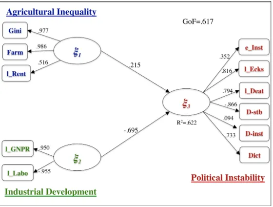
Parameter estimates are represented in figure 7. It is possible to inve-stigate the relations betweenAgricultural Inequality,Industrial Development and Political Instability through the path coefficients represented in the fi-gure; obviously, the two latent predictors impact in opposite sense on the response. However, Political Instability largely depends on Industrial Deve-lopment rather than on Agricultural Inequality. The higher the Industrial Development is, the lower the Political Instability is.
Figura 7: PLS-PM analysis of Russet data as transformed by Tenenhaus: model parameter estimates
As one can expect, the variablesgini, farm and l_rent are positively cor-related to the LV Agricultural Inequality. The LV Industrial Developmentis positively affected by the gross national product (variable l_gnpr) and ne-gatively affected by the percentage of agricultural workers (variable l_labo). All of the MVs of the block representingPolitical Instabilitypositively impact on the LV except for the binary variable d-stb, which indicates the countries with a stable democratic regime.
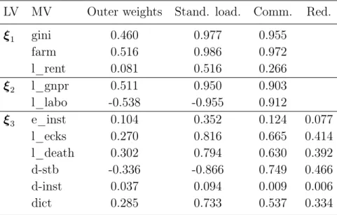
LV MV Outer weights Stand. load. Comm. Red. ξ1 gini 0.460 0.977 0.955 farm 0.516 0.986 0.972 l_rent 0.081 0.516 0.266 ξ2 l_gnpr 0.511 0.950 0.903 l_labo -0.538 -0.955 0.912 ξ3 e_inst 0.104 0.352 0.124 0.077 l_ecks 0.270 0.816 0.665 0.414 l_death 0.302 0.794 0.630 0.392 d-stb -0.336 -0.866 0.749 0.466 d-inst 0.037 0.094 0.009 0.006 dict 0.285 0.733 0.537 0.334
Tabella 3: PLS-PM analysis of Russet data as transformed by Tenenhaus: outer model results
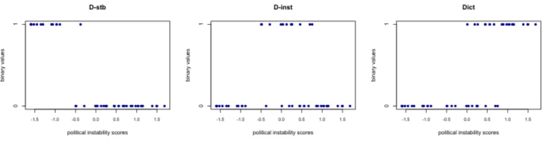
It is not clear if the overall weight of the variabledemo, expressed by the three dummy variables d-stb, d-inst and dict, is high or low. While weights of d-stb and dict are large, the weight of d-inst is almost zero (see table 3). As matter of fact the weight of the binary variable d-inst is so small just because there is a strong relation between the categorical variable demo and the LV Political Instability. In fact, the category d-stb is mainly associated with observations sharing the lowest values of the LV, while the category dict is mainly associated with observations sharing the highest values of the LV and the category d-instis mainly associated with observation sharing the central values of Political Instability score distribution. Hence, there is a strong relation between the LV and all of the binary variables representing the categories of MV demo. Unfortunately, while relations between binary variables dictand d-stb andPolitical Instabilityare pretty monotone (and so they can be easily approximated by a linear function), the binary variable d-inst is linked toPolitical Instabilityby a non-monotonic relation (see figure 8). As a consequence, this variable is underestimated in the model.
Figura 8: Raw values of binary variables corresponding to categories of variable demo plotted versus the LV Political Instability values
LV R2 Mean Comm. Mean Red.
ξ1 0.737
ξ2 0.908
ξ3 0.589 0.572 0.337
Tabella 4: NM-PLSPM analysis of Russet data as transformed by Tenenhaus (variable demo is analyzed at a nominal scaling level): model assessment
4.1 Model estimation with Non-Metric PLS Path Modeling In order to overcome the binary coding drawbacks, we perform a Non-Metric PLS-PM analyses on Russet data-set by using an R code developed by Rus-solillo [2009]. In this analysis, we leave metric variables as transformed by Tenenhaus while the non-metric variable demo will be properly quantified. The new model is represented in figure 9. Now the LV Political Instabilityis expressed by just four MVs: e_inst, l_ecks, l_deathand demo.
The quality of this model is summarized in table 4. With respect to the previous one, this model shows a worst prediction capability of the latent response, while it gains on the explicative capability of the MV underlying the concept of Political Instability. The mean Communalities of the other two blocks remain about the same. However, the global model fit improves, as GoF passes from 0.617 to 0.643.
The non-metric analysis makes it clear that the MV demo is the most important in the construction of the LV Political Instability (see table 5). According to these results we can conclude that the categories of the MV
Figura 9: NM-PLSPM analysis of Russet data as transformed by Tenenhaus (the variable demo is analyzed at a nominal scaling level): model parameter estimates
farm 0.502 0.984 0.968 l_rent 0.117 0.543 0.294 ξ2 l_gnpr 0.514 0.951 0.904 l_labo -0.536 -0.955 0.911 ξ3 e_inst 0.127 0.375 0.140 0.083 l_ecks 0.329 0.853 0.728 0.429 l_death 0.370 0.826 0.682 0.402 demo 0.427 0.859 0.739 0.435
Tabella 5: NM-PLSPM analysis of Russet data as transformed by Tenenhaus (variable demo is analyzed at a nominal scaling level): outer model results
demo are greatly discriminant with respect to thePolitical Instabilityscores. In fact, the weight of an MV quantified at a nominal scaling level reflects the variability of the corresponding LV explained by the categories of the MV. 5 Conclusion
Structural Equation Models, and mainly PLS Path Models, are very useful tools to compute composite and complex indicators. However, such models take into account only quantitative indicators. Until now, composite indica-tors have been obtained only as a mathematical combination of (quantitative) indicators [Saisanaet al., 2002]. Nevertheless, considering also categorical in-dicators in building composite inin-dicators is very fascinating. For instance, when computing complex and composite indicators, it could be interesting to take into account demographic variables, such as religion or gender, and/or categorical variables defining states, such as type of government. All these variables can play different roles: they can play the role of a manifest mo-derating categorical variable (such as the variable gender in computing the GDI index); they can define latent classes of units showing different systems of weights; or they can be used as categorical indicators in computing the composite indicators. In this work we discussed the use of SEMs to build systems of composite indicators. Moreover, we reviewed a suite of
statisti-cal methodologies for handling categoristatisti-cal indicators with respect to the role they play in a system of composite indicators.
References
Al-Nasser A. (2003), Customer satisfaction measurement models: Generali-zed maximum entropy approach, Pakistan Journal of Statistics, 19, 213-226. Amato S., Esposito Vinzi V., Tenenhaus M. (2005), A global goodness-of-fit index for PLS structural equation modeling, Technical report, HEC School of Managment, France.
Baron R.M., Kenny D.A. (1986), The Moderator-Mediator Variable Distinc-tion in Social Psychological Research: Conceptual, Strategic, and Statistical Considerations, Journal of Personality and Social Psychology,51 (6), 1173-1182.
Bollen K. A. (1989), Structural equations with latent variables, Wiley, New York.
Chin W. (1998), The partial least squares approach for structural equation modeling. In G. A. Marcoulides (ed.),Modern Methods for Business Resear-ch, Lawrence Erlbaum Associates, London, 295-236.
Chin W. (2003), A permutation procedure for multi-group comparison of PLS models, in PLS and related methods - Proceedings of the International Symposium PLS’03, M. Vilareset al. (eds), DECISIA, 33-43.
Chin W., Marcolin B., Newsted P. (2003), A partial least squares latent variable modeling approach for measuring interaction effects: results from a monte carlo simulation study and an electronical-mail emotion/adoption study, Information Systems Research, 14, 189-217.
Djkstra T. (1983), Some comments on maximum likelihood and partial least squares methods, Journal of Econometrics, 22, 67-90.
Efron B., Tibshirani R.J. (1993), An Introduction to the Bootstrap, Chap-man&Hall, New York.
Computational Statistics and Data Analysis, 18,121-140.
Esposito Vinzi V., Trinchera L., Squillacciotti S., Tenenhaus M. (2008), REBUS-PLS: A response - based procedure for detecting unit segments in PLS path modeling, Applied Stochastic Models in Business and Industry (ASMBI), 24 (5), 439-458.
Esposito Vinzi V., Trinchera L., Amato S. (2010) PLS Path Modeling: Recent Developments and Open Issues for Model Assessment and Improvement, in Handbook Partial Least Squares: Concepts, Methods and Applications, Com-putational Statistics Handbook series (Vol. II), V. Esposito Vinzi, W. Chin, J. Henseler and H. Wang (eds.) Springer-Verlag, Europe.
Fornell C., Bookstein F.L. (1982), Two structural equation models: LISREL and PLS appliead to consumer exit-voice theory, Journal of Marketing Re-search XIX, 440-452.
Gifu A. (1990), Nonlinear Multivariate Analysis, Chichester, UK: Wiley. Gorsuch R. L. (1983), Factor Analysis, Lawrence Erlbaum (2nd edition), Mahwah, New Jersey.
Hagerty M. R. , Cummins R.A, et al. (2001), Quality of Life for National Policy: Review and Agenda for Research. Social Indicators Research, 55 (1), 1-96.
Hahn C., Johnson M., Herrmann A., Huber F. (2002), Capturing Customer Heterogeneity using a Finite Mixture PLS Approach,Schmalenbach Business Review,54, 243-269.
Hall J. (2005), Measuring Progress – An Australian Travelogue, Journal of Official Statistics, 21 (4), 727-746
Henseler J., Fassot G. (2010), Testing moderating effects in PLS path mo-dels: An illustration of available procedure, in Handbook Partial Least Squa-res: Concepts, Methods and Applications, Computational Statistics Hand-book series (Vol. II), V. Esposito Vinzi, W. Chin, J. Henseler and H. Wang
(eds.) Springer-Verlag, Europe
Hoteling H. (1933), Analysis of a complex of statistical variables into princi-pal components, Journal of Educational Psychology, 24.
Hwang H., Takane Y. (2004), Generalized structured component analysis, Psychometrika, 69, 81-99.
Jöreskog K. (1970), A general method for analysis of covariance structure, Biometrika, 57, 239-251.
Jöreskog K., Sörbom D. (1979), Advances in Factor Analysis and Structural Equation Models, Abt Books.
Jöreskog K., Sörbom D. (1996),LISREL 8: Structural Equation Modeling wi-th wi-the SIMPLIS command Language, Scientific Software International, Hove and London.
Jöreskog K., Wold H. (1982), The ML and PLS techniques for modeling wi-th latent variables: historical and comparative aspects. In K. Jöreskog & H. Wold (eds), Systems Under Indirect Observation, Vol. Part I, North-Holland, Amsterdam, 263-270.
Kaplan D. (2000), Structural Equation Modeling: Foundations and Exten-sions, Sage Publications Inc., Thousands Oaks, California.
Kenny D., Judd C. (1984), Estimating the nonlinear and interactive effects of latent variables, Psychological Bulletin, 96, 201-210.
Lohmöller J. (1987), LVPLS program manual, version 1.8, Technical report, Zentralarchiv für Empirische Sozialforschung, Universität Zu Köln, Köln. Lohmöller J. (1989), Latent variable path modeling with partial least squares, Physica-Verlag, Heildelberg.
Lyttkens E., Areskoug B., Wold H. (1975), The convergence of NIPALS estimation procedures for six path models with one or two latent variables,
Technical report, University of Göteborg.
McLachlan G.J., Peel D. (2000),Finite Mixture Models, John Wiley & Sons, Inc., New York, Chichester, Weinheim, Brisbane, Singapore, Toronto. R Development Core Team (2009), R : A language and environment for sta-tistical computing, R Foundation for Stasta-tistical Computing, Vienna, Austria, ISBN 3-900051-07-0, URL http ://www.R-project.org.
Ringle C., Wende S., Will A. (2010), Finite mixture partial least squares analysis : Methodology and numerical examples, in Handbook Partial Lea-st Squares: Concepts, Methods and Applications, Computational StatiLea-stics Handbook series (Vol. II), V. Esposito Vinzi, W. Chin, J. Henseler and H. Wang (eds.) Springer-Verlag, Europe
Russet B. M. (1964), Inequality and instability, Word politics, 21, 422-454. Russolillo G. (2009), Partial Least Squares Methods for Non-Metric Data, PhD thesis, DMS, University of Naples.
Saisana M., Tarantola S. (2002), State-of-the-art Report on Current Metho-dologies and Practices for Composite Indicator Development, EUR 20408 EN, European Commission-JRC: Italy.
Tenenhaus M. (1998),La Régression PLS: théorie et pratique, Technip, Paris. Tenenhaus M., Amato S., Esposito Vinzi V. (2004), A global goodness-of-fit index for PLS structural equation modelling. InProceedings of the XLII SIS Scientific Meeting, Vol. Contributed Papers, CLEUP, Padova, 739-742. Tenenhaus M., Esposito Vinzi V., Chatelin Y.M., Lauro C. (2005), PLS path modeling, Computational Statistics and Data Analysis,48, 159-205.
Tenehaus M., Mauger E., Guinot C. (2010), Use of ULS-SEM and PLS-SEM to measure a group effect in a regression model relating two blocks of bi-nary variables, in Handbook Partial Least Squares: Concepts, Methods and Applications, Computational Statistics Handbook series (Vol. II), V.