arXiv:1909.04613v1 [cs.DS] 10 Sep 2019
Faster quantum and classical SDP approximations
for quadratic binary optimization
Fernando G.S L. Brand˜ao,1, 2 Richard Kueng1,2 and Daniel Stilck Fran¸ca3,4 1Institute for Quantum Information and Matter, California Institute of Technology,
Pasadena, CA, US
2Department of Computing and Mathematical Sciences, California Institute of Technology,
Pasadena, CA, US
3QMATH, Department of Mathematical Sciences, University of Copenhagen, Denmark 4Department of Mathematics, Technische Universit¨at M¨unchen, Germany
Abstract
We give a quantum speedup for solving the canonical semidefinite programming re-laxation for binary quadratic optimization. The class of rere-laxations for combinatorial optimization has so far eluded quantum speedups. Our methods combine ideas from quantum Gibbs sampling and matrix exponent updates. A de-quantization of the algo-rithm also leads to a faster classical solver. For generic instances, our quantum solver gives a nearly quadratic speedup over state-of-the-art algorithms. We also provide an effi-cient randomized rounding procedure that converts approximately optimal SDP solutions into constant factor approximations of the original quadratic optimization problem.
1
Introduction
Quadratic optimization problems with binary constraints are an important class of of opti-mization problems. Given a (real-valued) symmetricn×nmatrix Athe task is to compute maximize hx|A|xi subject to x∈ {±1}n (MaxQP). (1) This problem arises naturally in many applications across various scientific disciplines, e.g. image compression [OP83], latent semantic indexing [Kol98], correlation clustering [CW04, MMMO17] and structured principal component analysis, see e.g. [KT19a, KT19b] and ref-erences therein. Mathematically, MaxQPs (1) correspond to computing the ℓ∞→ ℓ1 norm
of A. This object is closely related to the cut norm (replace x ∈ {±1}n by x ∈ {0,1}n), an important concept in theoretical computer science [FK99, AFdlVKK03, AN06]. The problem of identifying the largest cut in a graph (MaxCut) is arguably the most prominent instance of aMaxQP. This membership highlights that optimal solutions of (1) areNP-hard to com-pute in the worst case. Despite their intrinsic hardness, quadratic optimization problems do
admit a canonicalsemidefinite programming (SDP) relaxation1 [GW95]:
maximize tr (AX) subject to diag(X) =1, X ≥0 (MaxQP SDP) (2) Here,X ≥0 indicates that then×nmatrixX is positive semidefinite (psd), i.e.hy|X|yi ≥0 for ally∈Rn. SDPs comprise a rich class of convex optimization problems that can be solved
efficiently, e.g. by using interior point methods [BV04].
Perhaps surprisingly, the optimal value of the MaxQP relaxation provides a constant factor approximation to the optimal value of the original quadratic problem. However, the associated optimal matrixX♯ is typicallynot in one-to one correspondence with an optimal feasible point x♯ ∈ {±1}n of the original problem (1). Randomized rounding procedures have been devised to overcome this drawback [GW95]. These transform X♯ into a binary vector ˜x ∈ {±1}n that achieves hx˜|A|x˜i ≥ γmaxx∈{±1}nhx|A|xi, with the optimal constant
γ = 2/π >0.63 [AN06].
Although tractable in a theoretical sense, the runtime associated with general purpose SDP solvers quickly becomes prohibitively expensive in both memory and time. This practical bottleneck has spurred considerable attention in the theoretical computer science community over the past decades [AHK05, BM05, BVB16, TYUC17]. (Meta) algorithms, like matrix multiplicative weights (MMW) [AHK05] solve the MaxQP SDP (2) up to additive error ǫ
in runtime O((n/ǫ)2.5s), where s denotes the column sparsity of A. Further improvements are possible, if the problem descriptionA has additional structure [AK16].
Very recently, a line of works pointed out that quantum computers can solve certain SDPs even faster [BS17, vAG18b, BKL+17, KP18]. However, current runtime guarantees de-pend on problem-specific parameters. These scale particularly poorly for most combinatorial optimization problems, including theMaxQP SDP, and negate any potential advantage.
In this work, we tackle this challenge and overcome shortcomings of existing quantum SDP solvers for the following variant of problem (2):
maximize tr 1 kAkAX (renormalized MaxQP SDP) (3) subject to hi|X|ii= n1 i∈[n], tr(X) = 1, X ≥0.
This renormalization of the original problem pinpoints connections to quantum mechanics: Every feasible point X obeys tr (X) = 1 and X ≥ 0, implying that it describes the state
ρ of a n-dimensional quantum system. In turn, such quantum states can be represented approximately by a re-normalized matrix exponential ρ = exp(−H)/tr(H), the Gibbs state
associated with Hamiltonian H. We capitalize on this correspondence by devising a meta algorithm –Hamiltonian Updates (HU) – that is inspired by matrix exponentiated gradient updates [TRW05], see also [LSW15, BKL+17, Haz06] for similar approaches. Although orig-inally designed to exploit the fact that quantum architectures can sometimes create Gibbs states efficiently, it turns out that this approach also produces faster classical algorithms.
1
Rewrite the objective function in (1) as tr (A|xihx|) and note that every matrixX=|xihx|withx∈ {±1}n
has diagonal entries equal to one and is psd with unit rank. Dropping the (non-convex) rank constraint produces a convex relaxation.
To state our results, we instantiate standard computer science notation. The symbolO(·) describes limiting function behavior , while ˜O(·) hides poly-logarithmic factors in the problem dimension and polynomial dependencies on the inverse accuracy 1/ǫ. We are working with the adjacency list oracle model, where individual entries and location of nonzero entries of the problem description A can be queried at unit cost. We refer to Section 3.4 for a more detailed discussion.
Theorem I (Hamiltonian Updates: runtime). Let A be a (real-valued), symmetric n×n matrix with column sparsity s. Then, the associated renormalized MaxQP SDP (3) can be solved up to additive accuracyǫin runtimeO˜ n1.5s0.5+o(1)poly(1/ǫ)on a quantum computer and O˜ min{n2s, nω}poly(1/ǫ) on a classical computer.
Here ω is the matrix multiplication exponent. The polynomial dependency on inverse accuracy is rather high (e.g. (1/ǫ)12 for the classical algorithm) and we intend to improve this scaling in future work. We emphasize that the quantum algorithm also outputs a classi-cal description of the solution. Already the classiclassi-cal runtime improves upon the best known existing results and we refer to Section 2.5 for a detailed comparison. Access to a quantum computer would increase this gap further. However, it is important to point out that The-orem I addresses the renormalizedMaxQP SDP (3). Converting it into standard form (2) results in an approximation error of order nkAkǫ. In contrast, MMW [AHK05] – the fastest existing algorithm – incurs an error proportional to ǫkAkℓ1. Importantly, this comparison is
favorable for generic problem instances, see Section 2.5.
The quantum algorithm outputs a classical description of an optimal HamiltonianH♯that encodes an approximately optimal, approximately feasible solutionρ♯= exp(−H♯)/tr exp(−H♯) of the renormalized MaxQP SDP (3). This classical output can subsequently be used for randomized rounding.
Theorem II (Rounding). Suppose that H♯ encodes an approximately optimal solution of
the renormalized MaxQP SDP (3) with accuracy ǫ. Then, there is a classical O˜(ns)-time randomized rounding procedure that converts H♯ into a binary vector x˜∈ {±1}n that obeys
2 π max x∈{±1}nhx|A|xi − O(nkAkǫ) ≤E[hx˜|A|x˜i]≤ max x∈{±1}nhx|A|xi+O(nkAkǫ).
This result recovers the best existing randomized rounding guarantees [AN06] in the limit of perfect accuracy (ǫ= 0). However, for ǫ > 0 the error scales with nkAk. In turn, randomized rounding only provides a multiplicative approximation if the objective value maxx∈{±1}nhx|A|xi is of the same order. This turns out to be the case for generic problem
instances and we refer to Section 2.5 for a more detailed discussion.
2
Detailed summary of results
We present Hamiltonian Updates – a meta-algorithm for solving convex optimization prob-lems over the set of quantum states based on quantum Gibbs sampling – in a more general setting, as we expect it to find applications to other problems. Throughout this work,k · ktr and k · kdenote the trace (Schatten-1) and operator (Schatten-∞) norms, respectively.
2.1 Convex optimization and feasibility problems
Most SDPs are a special instance of a more general class of convex optimization. For a symmetric matrix Aand closed convex sets C1, . . . ,Cn, solve
minimize tr (AX) (CPopt) (4)
subject to X∈ C1∩ · · · ∩ Cm, tr(X) = 1, X ≥0.
The constraint tr(X) = 1 enforces normalization, whileX≥0 is the defining structure con-straint of semidefinite programming. Together, they restrict X to the set of n-dimensional quantum statesSn={X: tr(X) = 1, X ≥0}. This quantum constraint implies fundamen-tal bounds on the optimal value: |tr(AX♯)| ≤ kAkkX♯ktr =kAk, according to Matrix H¨older [Bha97, Ex. IV.2.12]. Binary search over potential optimal valuesλ∈[−kAk,kAk] allows for reducing the convex optimization problem into a sequence of feasibility problems:
find X ∈ Sn (CPfeas(λ)) (5) subject to tr (AX)≤λ,
X ∈ C1∩ · · · ∩ Cm.
The convergence of binary search is exponential. This ensures that the overhead is benign: a total of log(kAk/ǫ) queries ofCPfeas(λ) suffice to determine the optimal solution ofCPopt
(4) up to accuracyǫ. In summary:
Fact 2.1. Binary search reduces the task of solving convex optimization problems (4) to the task of solving convex feasibility problems (5).
2.2 Meta-algorithm for approximately solving convex feasibility problems
We adapt a meta-algorithm developed by Tsuda, R¨atsch and Warmuth [TRW05], see also [LSW15, AK16, Haz06, BKL+17] for similar ideas. To this end, we require subroutines that
allow for testing ǫ-closeness (in trace norm) to each convex set Ci.
Definition 2.1 (ǫ-separation oracle). Let C be a closed, convex set. An ǫ-separation oracle (with respect to the trace norm) is a subroutine that either accepts a matrix X (if it is close to feasible), or provides a hyperplane P that separates ρ from the convex set:
OC,ǫ(X) =
(
accept X if minY∈CkX−Yktr ≤ǫ,
else: outputP s.t. kPk ≤1, tr(P(Y −X))≥ǫfor allY ∈ C.
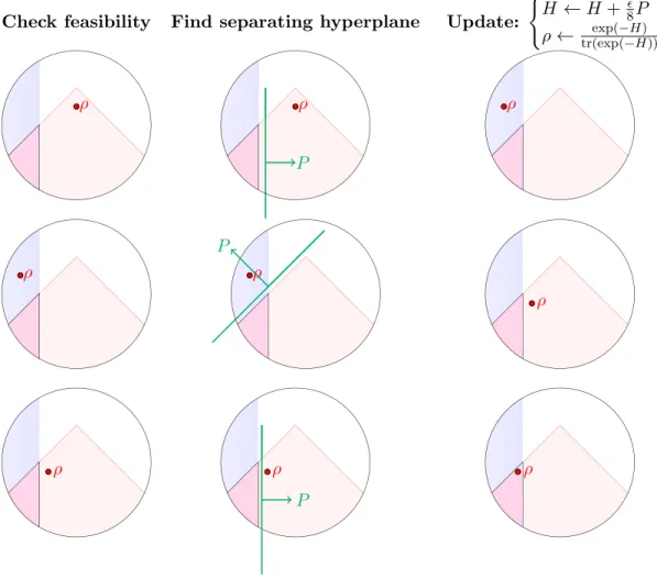
Hamiltonian Updates (HU) is based on a change of variables that automatically takes care of positive semidefiniteness and normalization: replace X in problem (5) by a Gibbs stateρH = exp (−H)/tr(exp(−H)). At each iteration, we queryǫ-separation oracles. If they all accept, the current iterate is ǫ-close to feasible and we are done. Otherwise, we update the matrix exponent to penalize infeasible directions: H→H+8ǫP, whereP is a separating hyperplane that witnesses infeasibility. This process is visualized in Figure 1 and we refer to Algorithm 1 for a detailed description.
Algorithm 1 Meta-Algorithm for approximately solving convex feasibility problems (5). Require: Query access to m ǫ-separation oracles O1,ǫ(·), . . . , Om,ǫ(·)
1: functionHamiltonianUpdates(T, ǫ)
2: ρ=n−1I and H= 0 ⊲ initialize the maximally mixed state
3: fort= 1, . . . , T do
4: fori= 1, . . . , mdo ⊲ Query oracles and check feasibility
5: if Oi,ǫ(ρ) =P then
6: H←H+8ǫP ⊲ Penalize infeasible direction
7: ρ←exp (−H)/tr(exp(−H)) ⊲ Update quantum state
8: break loop
9: end if
10: end for
11: return (ρ, H) and exit function ⊲Current iterate is ǫ-feasible
12: end for
13: end function
Theorem 2.1 (HU: convergence). Algorithm 1 requires at most T = ⌈16 log(n)/ǫ2⌉ + 1 iterations to solve a quantum feasibility problem (5). Otherwise, the problem is infeasible.
The proof follows from establishing constant step-wise progress in quantum relative entropy. The quantum relative entropy between any feasible state and the initial state
ρ0 = n−1I (maximally mixed state) is bounded by log(n). Therefore, the algorithm must
terminate after sufficiently many iterations. Otherwise the problem is infeasible. We refer To Section 3.1 for details.
Theorem 2.1 has important consequences: The runtime of approximately solving quantum feasibility problems is dominated by the cost of implementingm separation oracles Oi,ǫ and the cost associated with matrix exponentiation. This reduces the task of efficiently solving convex feasibility problems to the quest of efficiently identifying separating hyperplanes and developing fast routines for computing Gibbs states.
The latter point already hints at a genuine quantum advantage: quantum architec-tures can efficiently prepare (certain) Gibbs states [CS17, Fra18, KBa16, PW09, TOV+09, TOV+09, YAG12, vAGGdW17].
2.3 Classical and quantum solvers for the renormalized MaxQP SDP
For fixed λ ∈ [−1,1] the (feasiblity) MaxQP SDP is equivalent to a quantum feasibility problem: find ρ∈ Sn∩ Aλ∩ Dn where Aλ= X : tr AkAk−1X≥λ , Dn={X: hi|X|ii= 1/n, i∈[n]}.
The setAλ corresponds to a half-space, while Dn is an affine subspace with codimension n. The simple structure of both sets readily suggests two ideal separation oracles (ǫ= 0):
OAλ: check tr(AkAk−
1ρ)≤λand output P =AkAk−1 if this is not the case.
ODn: Check hi|ρ|ii= 1/n for all i∈[n] and output P =
Pn
i=1I{hi|ρ|ii>1/n} |iihi|if this is
not the case.
2.3.1 Classical runtime
For fixedρH = exp(−H)/tr(−H) both separation oracles are easy to implement on a classical computer. Hence, matrix exponentiation is the only remaining bottleneck. This can be mitigated by truncating the Taylor series for exp(−H) after l′ = O(log(n)/ǫ) many steps. Approximating ρ in this fashion only requires O(minn2s, nω log(n)ǫ−1) steps and only
incurs an error of ǫ in trace distance, see Section 3.3. The following result becomes an immediate consequence of Fact 2.1 and Theorem 2.1.
Corollary 2.1(Classical runtime for theMaxQP SDP). Suppose thatAhas row-sparsity s. Then, the classical cost of solving the associated (renormalized) MaxQP SDP up to additive errorǫ isO(min{n2s, nω}log(n)ǫ−12).
2.3.2 Quantum runtime
Quantum architectures can efficiently prepare (certain) Gibbs states and are therefore well suited to overcome the main classical bottleneck. In contrast, checking feasibility becomes more challenging, because information about ρ is not accessible directly. Instead, we must prepare multiple copies ofρ and perform quantum mechanical measurements to test feasibil-ity:
• O(ǫ−2) copies of ρ suffice toǫ-approximate tr(AkAk−1ρ) via phase estimation.
• O(nǫ−2) copies suffice with high probability to estimate the diagonal entries of ρ (up
to accuracyǫ in trace norm) via repeated computational basis measurements.
Combining this with the overall cost of preparing a single Gibbs state implies the following runtime for executing Algorithm 1 on a quantum computer. This result is based on thesparse oracle input model and we refer to Sec. 3.4 for details.
Corollary 2.2 (Quantum runtime for theMaxQP SDP). Suppose that A has row-sparsity s. Then, the quantum cost of solving the renormalized MaxQP SDP up to additive error ǫ isO˜(n1.5s0.5+o(1)poly(1/ǫ)).
The quantum solution corresponds to a classical description of an approximately opti-mal, approximately feasible Hamiltonian H♯ and the potential to produce samples from the associated approximately optimal Gibbs state ρ♯ = exp(−H♯)/tr exp(−H♯) in sub-linear runtime ˜O(√n) on a quantum computer.
2.4 Randomized rounding
The renormalizedMaxQP SDP(3) arises as a convex relaxation of an important quadratic optimization problem (1). However, the optimal solution X♯ is typically not of the form
Algorithm 2 Randomized rounding based on optimal Hamiltonian H♯
1: functionRandomizedRounding(H♯)
2: Draw a random vector g∈R
n with i.i.d. N(0,1) entries.
3: Computez=Plk=0 (−2Hkk♯!)kg forl=O(ǫ−1log(n)).
4: output xi = sign(zi).
5: end function
|xihx|, with x∈ {±1}n. Goemans and Williamson [GW95] established randomized rounding techniques that allow for converting X♯ into a cut x♯ that is close-to optimal. We show that this procedure is stable, i.e. randomized rounding of an approximately feasible, approx-imately optimal point still results in an approxapprox-imately optimal cut. Algorithm 2 executes this procedure while simultaneously truncating Taylor expansions of the matrix exponential to save runtime.
Proposition 2.1. Let H♯ be such that ρ♯ = exp(−H♯)/tr(exp(−H♯)) is an ǫ-approximate solution to the renormalized MaxQPSDP (3) with value α♯ = tr AkAk−1ρ♯. Then, the
(random) output x∈ {±1}n of Algorithm 2 can be computed inO˜(ns)-time and obeys 2
πnkAk
α♯− O(ǫ)≤Ehx|A|xi ≤nkAk(α♯+O(ǫ)).
This rounding procedure is fully classical and can be executed in runtime ˜O(ns). We refer to Sec. 3.5 for details. What is more, it applies to both quantum and classical solutions of theMaxQP SDP. Even the quantum algorithm provides H♯ in classical form, while the associatedρ♯is only available as a quantum state. Rounding directly withρ♯would necessitate a fully quantum rounding technique that, while difficult to implement and analyze, seems to offer no advantages over the classical Algorithm 2.
In [AN06] the authors prove that the constant π2 in Proposition 2.1 is optimal. Strictly speaking, this optimal constant only applies to psd problem descriptions A ≥ 0. However, the following simple trick converts anyMaxQPinput matrixA into a related matrix that is psd: A′ = kAkI A AT kAkI ≥0.
It is easy to verify that the associatedMaxQPand SDP relaxation values becomeα+2nkAk, where α is the optimal value corresponding to the original matrix A. This correspondence allows us to reduce the task of computing MaxQP (1) and its SDP relaxation (2) to psd matrices.
2.5 Comparison to existing work
TheMaxQP SDPhas already received a lot of attention in the literature. Table 1 contains a runtime comparison between the contributions of this work and the best existing classical results [AHK05, AK16]. This highlights regimes, where we obtain both classical and quan-tum speedups. In a nutshell, Hamiltonian Updates outperforms state of the art algorithms whenever the target matrix A has both positive and negative off-diagonal entries and the optimal value of the SDP scales asnkAk. It is worthwhile to explore the following examples.
Nearly quadratic quantum speedups and classical speedups for generic instances:
The conditions under which Hamiltonian Updates offers speedups are generic for matrices that have both positive and negative entries, see Appendix A. More precisely, suppose thatA
is a random matrix whose entries are i.i.d samples of a centered random variable with bounded fourth moment. Then, kAkℓ1 = Θ(n
3/2kAk) and kAk
1→∞ = Θ(nkAk) in expectation . This
implies that the runtime of Hamiltonian Updates improves upon MMW [AHK05]. For these dense instances, the MMW-runtime is ˜O(n3.5) compared to ˜O(n3) provided in Corollary 2.1 and ˜O(n2) in the quantum case. This is almost a quadratic quantum improvement in n.
Moreover, we expect it to be possible to obtain quadratic quantum speedups. It is easy to see that for assparse matrixA we havekAkℓ1 ≤nskAk. Fors-sparse matrices such that
kAk1→∞ = Θ(nkAk) andkAkℓ1 = Θ(nskAk) we then have the runtime ˜O(min{(ns)
2.5, n3s})
for MMW. It is then not difficult to see that identifying instances with this scaling and
s= Ω(n1/3) would lead to quadratic quantum speedups.
To the best of our knowledge, the quantum implementation of Hamiltonian updates es-tablishes the first quantum speedup for problems of this type. Corollary 2.2 eses-tablishes a nearly quadratic speedup for generic MaxQP SDP instances compared to current state of the art.
No speedups for MaxCut: Additional structure can substantially reduce the runtime of existing MMW solvers [AK16]. For weighted MaxCut, in particular, A is related to the adjacency matrix of a graph and has non-negative entries. This additional structure facilitates the use of powerful dimensionality reduction and sparsification techniques that outperform Hamiltonian Updates. However, these techniques do not readily apply to general problem instances, where the entries ofA can be both positive and negative (sign problem). We refer to Appendix B for a more detailed discussion.
Sherrington-Kirkpatrick Model: It is also interesting to take generic problem instances more seriously. SamplingA from the Gaussian ensemble (i.e. each entry is an i.i.d. standard normal random variable) produces an ensemble of MaxQP SDPs that is closely related to the Sherringkton-Kirkpatrick (SK) model [Pan13]. This problem has received considerable attention in the statistical physics literature. In particular, recent work [Mon18] shows that, under some unproven conjectures, it is possible to solve the quadratic optimization in (1) directly in time ˜O(n2). Furthermore, there is an integrability gap for the SDP relaxation of
this problem in the Gaussian setting [KB19].
Previous quantum SDP solvers: previous quantum SDP solvers [BS17, vAG18b, BKL+17]
with inverse polynomial dependence on the errror do not provide speedups for solving the
MaxQP SDP, as their complexity depends on a problem specific parameter, the width of the SDP. We refer to the aforementioned references for a definition of this parameter and for the complexity of the solvers under different input models and only focus on why none of them readily gives speedups for the problem at hand. As shown in [vAGGdW17, Theorem 24], the width parameter scales at least linearly in the dimensionnfor theMaxQP SDP. To the best of our knowledge, the solvers mentioned above have a dependence that is at least quadratic in the width and at least an12 dependence on the dimension. Thus, the combination of the
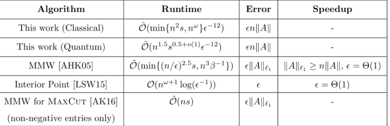
Algorithm Runtime Error Speedup This work (Classical) O˜(min{n2s, nω
}ǫ−12) ǫnkAk
-This work (Quantum) O˜(n1.5
s0.5+o(1) ǫ−12) ǫnkAk -MMW [AHK05] O˜(min{(n/ǫ)2.5s, n3β−1}) ǫkAkℓ 1 kAkℓ1≥nkAk,ǫ= Θ(1) Interior Point [LSW15] O(nω+1 log(ǫ−1)) ǫ ǫ= Θ(1)
MMW forMaxCut[AK16] O˜(ns) ǫkAkℓ
1
-(non-negative entries only)
Table 1: comparison of different classical algorithms to solve the original MaxQP SDP
(2). The speedup column clarifies in which regimes we obtain speedups and ω denotes the exponent of matrix multiplication. Here β corresponds to the value of MAXQP SDP multiplied bynkAk/kAkℓ1.
term stemming from the width and the dimension already gives a higher complexity than our solver. Moreover, enforcing the diagonial constraints in the renormalizedMAXQP SDP
in Eq. 3 in the straightforward way would require an error ǫ that is at most of order n−1. Given that these previous solvers also have a dependency on ǫ−1 that is at least quadratic,
previous quantum methods do not readily apply and have worse runtimes than available classical algorithms. In [KP18], the authors give a quantum SDP solver whose complexity is
e
Onξ22.5µκ3log ǫ−1
. Hereκandµare again problem specific parameters andξ is precision to which each constraint is satisfied. As noted before, a straightforward implementation of the MAXQP SDP requires ξ to be at most of order n−1, which establishes a runtime of
order at least n4.5 using those methods. Thus, we conclude that all current quantum SDP solvers do not offer speedups over state of the art classical algorithms, see Table 1 for more details.
Finally, we want to point out that subtleties regarding error scaling do not arise for
MaxCut. If A is the adjacency matrix of a d-regular graph on n vertices, then nkAk∞ =
nd=kAkℓ1 and the different errors in Table 1 all coincide.
3
Technical details and proofs
3.1 Proof of Theorem 2.1By construction, Algorithm 1 (Hamiltonian Updates) terminates as soon as it has found a quantum stateρ that is ǫ-close to being feasible. Correctly flagging infeasibility is the more interesting aspect of Theorem 2.1 (convergence to feasible point).
Lemma 3.1. Suppose Algorithm 1 does not terminate after T = ⌈16 log(n)/ǫ2⌉+ 1 steps. Then, the feasibility problem (5) is infeasible.
Proof. By contradiction. Suppose there exists a feasible pointρ∗in the intersection of allm+1 sets and we ran the algorithm for T steps. Instantiate the short-hand notation ρt = ρHt =
Check feasibility Find separating hyperplane Update: ( H ←H+8ǫP ρ← tr(exp(exp(−−HH))) ρ ρ P ρ ρ PS ρ ρ ρ ρ P ρ
Figure 1: Caricature of Hamiltonian Update iterations in Algorithm 1: Schematic illustration of the intersection of three convex sets (i) a halfspace (blue), (ii) a diamond shaped convex set (red) and (iii) the set of all quantum states (clipped circle). Algorithm 1 (Hamiltonian Updates) approaches a point in the convex intersection (magenta) of all three sets by itera-tively checking feasibility (left column), identifying a separating hyperplane (central column) and updating the matrix exponent to penalize infeasible directions (right column).
exp(−Ht)/tr(exp(−Ht)) for the t-th state and Hamiltonian in Algorithm 1. Initialization withH0 = 0 andρ0 =I/nis crucial, as it implies that the quantum relative entropy between ρ∗ and ρ0 is bounded:
S(ρ∗kρ0) = tr (ρ∗(logρ∗−logρ0))≤log(n).
We will now show that the relative entropy between successive (infeasible) iterates ρt+1, ρt and the feasible state ρ∗ necessarily decreases by a finite amount. Let Pt be the hyperlane
that separatesρt from the feasible set. The update ruleHt+1=Ht+8ǫPt then asserts
S(ρ∗kρt+1)−S(ρ∗kρt) =tr (ρ∗(Ht−Ht1)) + log tr (exp(−Ht+1)) tr (exp(−Ht)) =−8ǫtr (Ptρ∗)−log tr exp −Ht+1+8ǫPt tr (exp(−Ht+1)) ! .
The logarithmic ratio can be bounded using the Peierls-Bogoliubov inequality [AL70, Lemma 1]: log (tr (exp(F+G)))≥tr (Fexp(G)) provided that tr (exp(G)) = 1. This implies
log tr exp −Ht+1+ ǫ 8Pt tr (exp(−Ht+1)) !
=−log tr exp Ht+1+8ǫPt−log (tr (exp(−Ht1)))I
≤tr 8ǫPtexp (Ht+1−log(tr (exp(Ht+1)))I)
=8ǫtr (Ptexp(−Ht+1)/tr (exp(−Ht+1))) = ǫ8tr (Ptρt+1).
Next, note that the updates are mild in the sense thatρt+1 andρtare close in trace distance. [BS17, Lem. 16] implies kρt1 −ρtktr ≤ 2 exp(
ǫ
8kPtk)−1
≤ 2ǫ, because kPtk ≤ 1 by
con-struction and we can also assume 8ǫ ≤log(2). Combining these insights with Matrix H¨older [Bha97, Ex. IV.2.12] ensures
S(ρ∗kρt+1)−S(ρ∗kρt)≤ −8ǫtr (Ptρ∗) +ǫ8tr (Ptρt+1)
=8ǫ(tr (Pt(ρt+1−ρt))−tr (Pt(ρt−ρ∗))) ≤8ǫ(kPtkkρt+1−ρtktr+ tr (Pt(ρt−ρ∗))).
The first contribution is bounded by2ǫkPtk ≤ 2ǫ, while Definition 2.1 ensures tr (Pt(ρt−ρ∗))≤ −ǫ(ρ∗ is feasible andPt is anǫ-separation oracle for the infeasible point ρt). In summary,
S(ρ∗kρt+1)−S(ρ∗kρt)≤ 8ǫ ǫ2−ǫ
=−16ǫ2 for all iterations t= 0, . . . , T
and we conclude S(ρ∗kρT) = T X t=0 (S(ρ∗kρt+1)−S(ρ∗kρt)) +S(ρ∗kρ0)≤ −Tǫ 2 16+ log(n).
This expression becomes negative as soon as the total number of stepsTsurpasses 16 log(n)/ǫ2. A contradiction, because quantum relative entropy is always non-negative.
3.2 Stability of the relaxed MaxQP SDP
Note that even if Algorithm 1 accepts a candidate point, it does not necessarily mean that this point is exactly feasible. Theorem 2.1 only asserts that this point is ǫ-close to all sets of interest. For the MaxQP SDP (3), this means that the outputs of the algorithm will only satisfy the diagonal constraints approximately and, in principle, the value of this further relaxed problem could differ significantly from the original value. In the next proposition we show that this is not the case:
Proposition 3.1. Let αǫ be the value attained by an approximately optimal, approximately
feasible – up to accuracy ǫ– solution to the MaxQP SDP (3) with input matrix A. Then,
|αǫ4nkAk −α|=O(ǫnkAk) where α is the true optimal value of the original SDP (2).
Proof. Letρbe a solution to the relaxedMaxQP SDP(3) with relaxation parameterǫ4. We will now construct an exactly feasible pointρ♯ of the MaxQP SDP(3). This modifications are mild enough to ensure that the associated SDP value will only change byO(ǫnkAk). We proceed in two steps: (i) ρ 7→ ρ′: Identify diagonal entries that substantially deviate from 1/nin the sense that|hi|ρ|ii −1/n|> ǫ2/n. Subseqently, replaceρ
iiby 1/nand set all entries in the i-th row and i-th column to zero. This ensures that ρ′ remains positive semidefinite.
(ii)ρ′→R: Replace all remaining entries by 1/n. This may thwart positive semidefiniteness, but the following convex combination restores this feature:
ρ♯ = 1+1ǫ2
R+ǫn2I.
By construction, this matrix is both psd and obeyshi|ρ♯|ii= 1/nfor all i∈[n]. In words: it is a feasible point of the renormalized MaxQP SDP(3).
We now show that these reformulations are mild. To this end, letB ={i: hi|ρ|ii −1/n} ⊂
[n] be the indices associated with large deviations. Without loss of generality, we can assume that these are the first|B|indices. Then,
kρ′−ρk1= n−1IB 0 0 ρ22 − ρ11 ρ12 ρ21 ρ22 1 = n−1IB−ρ11 −ρ12 −ρ12 0 tr ≤kρ11ktr+ 2kρ12ktr+kn−1IBktr. (6)
Next, note that ǫ4-approximate feasibility impliesPni=1(|hi|ρ|ii −1/n|)≤ǫ4. This, in turn, demands|B|ǫn2 ≤ǫ4 or, equivalently |B| ≤nǫ2. The definition ofB moreover asserts
kρ22ktr ≥(n− |B|)1−ǫ
2
n ≥(1−ǫ2)2. Moreover, as shown in [Kin03], we have
kρ11ktr kρ12ktr kρT 12ktr kρ22ktr tr ≤ ρ11 ρ12 ρT 12 ρ2 tr =kρktr = tr(ρ) = 1.
Ask · ktr ≥ k · k2 (the Frobenius, or Schatten-2 norm), it follows from the last equation that
And, as kρ22k2tr ≥(1−ǫ2)4, we conclude kρ11k2tr+ 2kρ12ktr2 = O(ǫ2).which in turn implies kρ11ktr+ 2kρ12ktr =O(ǫ). Inserting this relation into Eq. (6) yields
kρ′−ρktr =O(ǫ).
Next, note that we obtainR from ρ′ by just replacing all diagonal entries ofρ′ by 1/n. This matrix is not necessarily positive semidefnite, but as all diagonals of ρ′ are in the range
(1±ǫ2)/n, it is easy to see that the matrixR+ ǫ2
nI is psd and has diagonal entries equal to 1 +ǫ2/n. Thus,ρ# is a feasible point of the renormalizedMaxQP SDP(3). It is easy to see that
trAnρ♯= 1+nǫ2
tr (AR) + ǫn2tr (A).
Now note that
tr (AR)−tr Aρ′≤ ǫn2 X i |Aii| ! ,
as these two matrices only differ on the diagonal, and there by at mostǫ2/n. Since n1 P i | Aii| ≤ kAk, we conclude that trAnρ♯−tr Anρ′=O ǫ2(1 +ǫ2)−1nkAk=O(ǫnkAk).
The claim then follows from combining triangle and (matrix) H¨older inequality:
tr (nAρ)−tr nAρ′≤nkAkkρ−ρ′ktr =O(nkAkǫ).
The above proof technique is constructive and allows us to construct a feasible point from an approximately feasible one inO(n2) time.
3.3 Approximately solving to the MaxQP SDP on a classical computer
We will now show how to use Hamiltonian Updates (Algorithm 1) to solve the MaxQP SDP(3) on a classical computer. It turns out that the main classical bottleneck is the cost of computing matrix exponentials ρ = exp(−H)/tr (exp(−H)). The following result asserts that coarse truncations of the matrix exponential already yield accurate approximations.
Lemma 3.2. Fix a Hermitian n×nmatrix H, an accuracy ǫand let l be the smallest even number that obeys (l+ 1)(log(l+ 1)−1) ≥ 2kHk+ log(n) + log(1/ǫ). Then, the truncated matrix exponential Tl=Plk=0k1!(−H)k is guaranteed to obey
exp(−H) tr(exp(−H))− Tl tr(Tl) tr ≤ǫ.
Proof. First note, that truncation at an even integerlensures thatTlis positive semidefinite. This is an immediate consequence of the fact that even-degree Taylor expansions of the (scalar) exponential are non-negative polynomials. In particular, kTlktr = tr (Tl). Combine this with tr (X)≤ kXktr ≤nkXk for all Hermitiann×nmatrices to conclude
exp(−H) tr (exp(−H))− Tl tr (Tl) tr ≤ 1 tr (exp(−H))kexp(−H)−Tlktr+ |tr (exp(−H))−tr (Tl)| tr (Tl) tr (exp(−H)) k Tlktr ≤2kexp(−H)−Tlktr
tr (exp(−H)) ≤2nexp(kHk)kexp(−H)−Tlk,
where we have also used tr (exp(−H))≥ kexp(−H)k ≥ exp(−kHk). By construction, both exp(−H) and Tl commute and are diagonal in the same eigenbasis. Let λ1, . . . , λn be the eigenvalues ofH. Then, Taylor’s remainder theorem asserts
kexp(−H)−Tlk= max 1≤i≤n exp(−λi)− l X k=0 1 k!(−λ)k ≤ maxiexp (−λi) (l+ 1)! ≤ exp(kHk) (l+ 1)! . The value ofl is chosen such that
2nexp(2kHk)
(l+ 1)! ≤exp(2kHk+ log(2) + log(n)−1−(l+ 1)(log(l+ 1)−1))≤ǫ, because (l+ 1)!≥e ((l+ 1)/e)l+1.
Corollary 3.1. Given an s sparse, symmetric n×n matrix A and ǫ > 0, we can solve the MaxQP SDP(3) up to an additive error O(ǫnkAk) in time O˜(min{n2s}, nω}ǫ−12) in a classical computer.
Although the dependency in ǫ for our algorithm is high, we expect that a more refined analysis of the error could improve this significantly. It is also possible to classically convert approximately feasible points (i.e. Pni=1|hi|ρ|ii −1/n| ≤ ǫ) into exactly feasible points (i.e. hi|ρ˜|ii = 1/n for alli∈[n]) while simultaneously only incurring a modest loss of O(nkAkǫ) in optimality. This conversion is an immediate consequence of the proof strategy behind Proposition 3.1.
Proof. As each run of Algorithm 1 takes time ˜O(1), we only need to implement the required oracles in time ˜O(n2sǫ−1) to establish the advertised runtime. First, note that the operator norm kHtk only grows modestly with the number of iterations t = 0, . . . , T. This readily follows fromH0 = 0, andkHt+1−Htk ≤ ǫ8kPtk ≤ 8ǫ. What is more, the maximal number of steps isT =⌈16 log(n)/ǫ2⌉, implying kHtk ≤2 log(n)ǫfor all t.
In turn, Lemma 3.2 implies that computing the Taylor series of exp(−Ht) up to a term of orderO(log(n)/ǫ) suffices to compute a matrix ˜ρt that is ǫ-close to the true iterate ρt = exp(−Ht)/tr (exp(−Ht)) in trace distance. Now note that the complexity of multiplying any matrix withHtis O(min{n2s}, nω}), asHt is a linear combination of a diagonal matrix and
A. Thus, we conclude that computing ˜ρttakes timeO(n2slog(n)ǫ−1). Checking the diagonal constraints then takes time O(n) and computing tr AkAk−1ρ˜
t
suffices to implement bothǫ-separation oracle and highlights that the runtime is dominated by computing approximations of the matrix exponential.
Finally, we show in Proposition 3.1 that in order to ensure an additive error of order O(ǫnkAk) for theMaxQP SDP, it suffices to solve the relaxed one up to an errorǫ4, from
which the claim follows.
3.4 Approximately solving to the MaxQP SDP on a quantum computer
We will now show how to implement ǫ-separation oracles on a quantum computer. As dis-cussed before, implementing the oracle requires us to evaluate the diagonal of the sequence of Gibbs statesρ= exp(−H)/tr (exp(−H)) and the value of tr ρAkAk−1. These two tasks
can be performed easily on a quantum computer given the ability to prepare copies of the quantum stateρ.
Lemma 3.3. We can implementǫ-separation oracles for the MaxQP SDP(3)on a quantum computer given access to O(nǫ−2) copies of the the input state ρ and the ability to measure tr(Aρ)kAk−1. Moreover, the classical postprocessing time needed to implement the oracle is
O(nǫ−2).
Proof. We implement the oracle by first measuring O(nǫ−2) copies of the input ρ in the
computational basis. This is enough to ensure that with probability of failure at mostO(e−n) the resulting empirical distribution of the measurement outcomes, ˆp=Pipˆ(i)|iihi|, satisfies
kX
i
hi|ρ|ii|iihi| −pˆktr ≤
ǫ
2.
IfkI/n−pˆktr ≤ 2ǫ, then the oracle for the diagonal constraints accepts the current state. If not, we output P =PiI{pˆi>1/n} |iihi|.This step requires a classical postprocessing time
of orderO(nǫ−2). For implementing the second oracle, we simply measureAkAk−1 directly.
A total of O(ǫ−2) copies of ρ suffice to determine tr AkAk−1ρ up to precision ǫ via phase
estimation [NC00].
Lemma 3.3 reduces the task of implementing separation oracles to the task of preparing independent copies of a fixed Gibbs state. There are many different proposals for prepar-ing Gibbs states on quantum computers [CS17, Fra18, KBa16, PW09, TOV+09, TOV+09, YAG12, vAGGdW17]. Here, we will follow the algorithm proposed in [PW09]. This ap-proach allows us to reduce the problem of preparing ρH = exp(−H)/tr (exp(−H)) to the task of simulating the Hamiltonian H. More precisely,[PW09, Appendix] highlights that
˜
O √nǫ−3 invocation of a controlledU, whereU satisfies
kU −eit0H
k ≤ O(ǫ3) where t0=π/(4kHk)
suffice to produce a state that isǫclose in trace distance to ρH. The probability of failure is at most n−1/ǫǫ2. We expect that a more refined analysis can lead to a better dependence on
the errorǫ. The methods presented in [vAGGdW17] seem like a good starting point for such future improvements. Here, however, we prioritize the scaling in the problem dimension n
By construction, the Hamiltonians we wish to simulate are all of the formH=aAkAk−1+ bD, where a, b = O(log(n)ǫ−1) and D is a diagonal matrix with bounded operator norm
kDk ≤ 1. It follows from [CW12, Theorem 1] that ˜Otexp(1.6plog log(n)tǫ−1) separate
simulations ofaAand bDsuffice to simulate H for timetup to an errorǫ. Thus, we further reduce the problem of simulating H to simulating A andD separately.
At this point it is important to specify input models for the matrix A, the problem description of theMaxQP SDP. We will work in thesparse oracle input model. That is, we assume to have access to an oracle Osparse that gives us the position of the nonzero entries.
That Given indices i for a column of A and a number 1≤ j ≤s, where A is s-sparse, the oracle acts as:
Osparse|i, ji=|i, f(i, j)i.
Heref(i, j) is thej−th nonzero element of thei−th column ofA. Moreover, we assume that the magnitude of individual entries are also accessible by means of another oracle:
OA|i, j, zi=|i, j, z⊕(AijkAk−1)i, Here, the entry AkAk−1
ij is represented by a bit string long enough to ensure the desired precision. The results of [Low19] then highlight that it is possible to simulate exp(itAkAk−1)
in timeO(t√skHk)1+o(1)ǫo(1).
Let us now turn to the task of simulating diagonal HamiltoniansD. LetOD be the matrix entry oracle for D. We suppose that it acts on Cn⊗ C2⊗m, where m is large enough to
represent the diagonal entries to desired precision in binary, as
OD|i, zi 7→ |i, z⊕Diii. (7)
It is then possible to simulate H =D for times t= ˜O(ǫ−1) with ˜O(1) queries to the oracle OD and elementary operations [BACS07]. Thus, efficient simulation of e−iDt follows from an efficient implementation of the oracle OD. The latter can be achieved with a quantum RAM [GLM08]. We consider the quantum RAM model from [Pra14]. There, it is possible to make insertions in time ˜O(1). Thus, given a classical description of a diagonal matrixD, we may update the quantum RAM in time ˜O(n). After we have updated the quantum RAM, we may implement the oracleOD in time ˜O(1). Combining all these subroutines establishes the second main result of this work.
Corollary 3.2. Given ans-sparse, symmetricn×nmatrixA(with appropriate oracle access) andǫ >0, we can solve the renormalized MaxQP SDP (3)up to an additive errorǫin time
˜
On1.5(√s)1+o(1)on a quantum computer.
Proof. It follows from Theorem 3.3 that producing ˜O(n) copies of Gibbs states suffices to implement the oracle. The results of [PW09] then imply that this can be done with ˜O(√n) Hamiltonian simulation steps, which, as discussed above, can be done in time ˜On0.5(√s)1+o(1).
3.5 Randomized rounding
As pioneered by the seminal work of Goemans and Williamson [GW95], it is possible to use randomized rounding techniques to obtain an approximate solution to the original quadratic optimization problem (1). These solutions are in expectation withinin a multiplicative factor of the value of the SDP relaxation (3) and the exact constant depends on the structure of the matrix A . We will explore Rietz’s method, as in [AN06], to show that it is possible to perform the rounding on a classical computer with our solutions to the approximateMaxQP SDPand still obtain good approximations. First, recall that the rounding algorithms usually work by first multiplying a random Gaussian vector by the square root of the solution. The approximate solution is then given by the signs of this random vector. Note that both classical and quantum algorithms output a classical description of the HamiltonianH♯associated with an approximately optimal, approximately feasible Gibbs state ρ♯ to (3). Pseudocode for the rounding algorithm is provided in Algorithm 2. The first important proof ingredient is an adaptation of [AN06, Eq. (4.1)].
Lemma 3.4. Fix v, w ∈ Rn (non-zero) and let g ∈ Rn be a random vector with standard normal entries. Then,
π 2E[sign(hv, gi)sign(hw, gi)] (8) =h v kvk,kwwki+E h h v kvk, gi − q π 2sign h v kvk, gi hkwwk, gi − q π 2sign h w kwk, gi i . Proof. In [AN06, Eq. (4.1)] the authors use rotation invariance to establish this identity for
two unit vectors. The claim then follows from observing that the distribution of sign(hv, gi)sign(hw, gi) is invariant under scaling both v and w by non-negative numbers. In particular,v 7→v/kvk
and w7→w/kwkdoes not affect the distribution.
The next step involves a technical continuity argument.
Lemma 3.5. Fix ǫ >0 and let ρ be a quantum state s.t.:
kX
i
hi|ρ|ii|iihi| −I/nktr ≤ǫ4
Define the set B ={i∈ [i] : ρii−1n
> ǫn2} and let ρB¯ be the submatrix with indices in the complement B¯ of B. Then, the matrix σ with entries σij = n√ρρijiiρjj is a quantum state that
obeys kρB¯ −σB¯ktr ≤3ǫ.
Proof. Note that σB¯ =D(ρB¯),where D is the linear map given by D(X) =DB¯XDB¯ and DB¯ is a|B¯| × |B¯|diagonal matrix with entries√nρii−1 fori∈B¯. This implies
kρB¯−ρB¯ktr =k(id− D) (ρBC)ktr ≤ kid− Dktr→trkkρB¯ktr ≤ kid− Dk∞→∞,
because kρB¯ktr ≤ kρktr = tr(ρ) = 1. Duality of norms and the fact that both id and D are self-adjoint with respect of the Frobenius inner product tr XTY implieskid−Dk+∞→+∞=
that all the entries of DB¯ are in 1±ǫ. Write DB¯ =I+Dǫ, whereDǫ is a diagonal matrix with entries that are bounded byǫin absolute value. Then,
id− D(X) =DǫX+XDǫ+DǫXDǫ for any matrix X. Submultiplicativity of the operator norm then implies
kDǫX+XDǫ+DǫXDǫk∞≤2kDǫk∞kXk+kDǫk2∞kXk∞≤3ǫkXk∞.
and, in turn,kid− Dk+∞→+∞≤3ǫ.
We are now ready to prove the main stability result required for randomized rounding.
Theorem 3.1. Let ρ♯ be an approximately feasible, optimal point of (3)with accuracyǫ4>0 and input matrixA. Letv1, . . . , vnbe the columns of
p
ρ♯, sampleg∈Rnwith i.i.d. Gaussian entries and setxi=sign(hvi, gi). Then,
trρ♯An+O(ǫnkAk)≥X i,j AijE(xixj)≥ 2 πtr ρ♯An− O(ǫnkAk)
Proof. The upper bound follows immediately from the fact MaxQP SDP (2) relaxations (renormalized or not) provide upper bounds to the original problem (1). The factors nkAk
is an artifact of the renormalization (3).
For the lower bound, we once more define B = {i ∈ [i] : |ρii−1/n| ≥ ǫ2/n} ⊂ [n]. Plugging invi andvj in (8), multiplying both sides byAij and summing over i, j implies
π 2 X i,j AijE(xixj) =n X i,j Aij(σij +τij) with σij = n√ρρijiiρjj and τij =E h h vi kvik, gi − q π 2sign h vi kvik, gi h vj kvjk, gi − q π 2sign h vj kvjk, gi i .
Following the same proof strategy as in [AN06, Sec. 4.1], we note that the matrixT defined by [T]ij = τij is a Gram matrix and, thus, psd. As we mentioned before, we may assume w.l.o.g. thatA is psd. We can then readily conclude
nX
i,j
Aijτij =ntr (AT)≥0,
because Frobenius inner products of psd matrices are always non-negative. We now have to relate tr (ρA) with tr (σA). To do so, we can argue like in Proposition 3.1 and see that tr (σ11),tr (ρ11) =O(ǫ2) (these correspond to the |B| × |B|psd submatrices with entries in B only). As bothσ and ρ are states, we conclude
kρ12ktr,kσ12ktr =O(ǫ)
by reusing the analysis provided in the proof of Proposition 3.1. Thus, it follows from H¨olders inequality and Lemma 3.5 that
tr (A(ρ−σ)) =tr (A(ρ22−σ22)) + tr (A(ρ11−2ρ12−σ11−2σ12))
=kAk(kσ22−ρ22ktr+kρ11ktr+ 2kρ12ktr+ 2kσ11ktr+ 2kσ12ktr) =O(kAkǫ), from which the claim follows.
Proposition 3.1 highlights that performing the rounding with approximate solutions to the
MaxQP SDP (3) still ensures a good approximate solution in expectation. But computing
p
ρ♯g = exp(−H/2)g/ptr (exp(−H)) directly stilll remains expensive because of matrix exponentiation. We will surpass this bottleneck by truncating the Taylor series of the matrix exponential in a fashion similar to Lemma 3.2. The following standard anti-concentration result for Gaussian random variables will be essential for this argument.
Fact 3.1. Let X be a N(0, σ2) random variable. Then P(|X| ≤σǫ) =O(ǫ).
Lemma 3.6. Let ρ♯ with associated Hamiltonian H♯ be an approximately optimal solution to the MAQP SDP (3) with kH♯k = O(log(n)/ǫ). Set S
l = Plk=0 k1!(−H♯/2)k with l =
O(log(n)/ǫ). Then, a random vector g∈Rn with standard normal entries obeys signheH♯/2g
i
i
=sign[(Slg)i] for all i∈[n] such that
ρ♯ii−n1< nǫ with probability at least 1− O(ǫ−1).
Note that the design of Algorithm 1 ensures that optimal Hamiltonians always obey kH♯k=O(log(n)/ǫ).
Proof. Define h = exp(−H♯/2)g and note that this is a Gaussian random vector with co-variance matrix exp(−H♯). LetB =i: |ρii−1/n|> nǫ ⊂[n] denote the set of indices for which ρii deviates substantially from 1/n. Then, every entry of h that is not contained in this index set obeys
[h]i = [exp(−H/2)g]i∼ N 0,nctr(exp(−H)) with c∈(1−ǫ,1 +ǫ).
The assumption kH♯k=O(log(n)/ǫ) ensures tr(exp(−H♯))/n ≥n−c′/ǫ−1 for some constant
c′. We can combine this with Fact 3.1 (Gaussian anti-concentration) to conclude
Ph|[h]
i| ≤n−2−c
′/(2ǫ)i
=O(1/n2) for all i∈B¯= [n]\B.
A union bound then asserts
P
h
∃i∈B¯ : |[h]i| ≤n−2−c′/ǫi=O(1/n).
Moreover, it follows from standard concentration arguments that
Phn−n14 ≤ kgk2 ≤n+n 1 4
i
≥1−2e−√n/8.
Thus, with probability at least 1− O(n−1), we have thatkgk2 ≤n+n14 and|[h]
i| ≥n−2−c
′/ǫ
for every entry i∈B¯. Following the same proof strategy as in Lemma 3.2, it is easy to see that by pickingl=O(ǫ−1log(n)) suffices to ensure that
kSl−exp(−H/2)k ≤n−4−
c′
2ǫ
Conditioning on the events emphasized above, implies max
i∈[n]|[(exp(−H/2)−Sl)g]i| ≤ k(exp(−H/2)−Sk)gk ≤ kexp(−H/2)−Skkkgk ≤n
This in turn ensures max
i∈B¯ |[(exp(−H/2)−Sl)g]i| ≤n
−3−c′
2ǫ, and in turn
sign ([h]i) = sign ([(exp(−H/2)g)]i) = sign ([Skg]i) for all i∈B,¯ because conditioning ensures|[exp(−H/2)g]i| ≥n−2−c2′ǫ.
Combining the statements we just proved we conclude that:
Proposition 3.2(Restatement of Proposition 2.1). Letǫ >0andAa real, symmetric matrix be given. Moreover, letH be the solution Hamiltonian to the relaxed MaxQP SDP(3) with error paramater ǫ4 and α∗ its value. Then, with probability at least 1−n−1, the output x of Algorithm 2 satisfies: nkAk(α∗+O(ǫ))≥E X ij Aijxixj≥ 2 πnkAk(α ∗− O(ǫ)), (9)
Proof. It follows from Lemma 3.6 that the output of Algorithm 2 will only differs from the vector obtained by performing the rounding with the approximate solution on a set of size O(nǫ) with probability at least 1−n−1. This can only change the value by at mostO(ǫnkAk). As Theorem 3.1 asserts that performing the rounding with the approximate solution is enough to produce a sign vector that satisfies (9) in expectation, this yields the claim.
Thus, we conclude that the rounding can be performed in time ˜O(ns) on a classical computer, as multiplying a vector with H takes time ˜O(ns) and we only need to perform this operations a logarithmic number of steps. Asns≤n1.5√s fors≤n, we conclude that
the cost of solving the relaxedMaxQP SDP (3) dominates the cost of rounding.
4
Conclusion and Outlook
By adapting ideas from [TRW05, Haz06, LSW15, BKL+17], we have provided a general
meta-algorithm for approximately solving convex feasibility problems with psd constraints.
Hamiltonian Updates is an iterative procedure based on a simple change of variables: rep-resent a trace-normalized, positive semidefinite matrix as X = exp(−H)/tr (exp(−H)). At each step, infeasible directions are penalized in the matrix exponent until an approximately feasible point is reached. This procedure can be equipped with rigorous convergence guaran-tees and lends itself to quantum improvements: X = exp(−H)tr (exp(−H)) is a Gibbs state
and H is the associated Hamiltonian. Quantum architectures can produce certain Gibbs states very efficiently.
We have demonstrated the viability of this approach by considering semidefinite program-ming relaxations of quadratic problems with binary constraints (MaxQP SDP) (2). The motivation for considering this practically important problem class was two-fold: (i)MaxQP SDPs have received a lot of attention in the (classical) computer science community. Powerful meta-algorithms, like matrix multiplicative weights [AK16], have been designed to solve these SDPs very quickly. (ii) Existing quantum SDP solvers [BS17, vAG18b, BKL+17, KP18] do
solvers depends on problem-specific parameters that scale particularly poorly for MaxQP SDPs.
The framework developed in this paper has allowed us to address both points. Firstly, we showed that a classical implementation of Hamiltonian Updates already improves upon the best existing results. A runtime of ˜O(n2s) suffices to find an approximately optimal solution. Secondly, we have showed that quantum computers do offer additional speedups. A quantum runtime of ˜O(n1.5s0.5+o(1)) is sufficient. We emphasize that this is the first quantum speedup for the practically important class of MaxQP SDPrelaxations. Subsequently, we have also devised a classical randomized rounding procedure that converts both quantum and classical solutions into close-to-optimal solutions of the original quadratic problem.
We note in passing that our algorithm is very robust, in the sense that it only requires the preparation of Gibbs states up to a constant precision, computational basis measurements and the ability to estimate the expectation value of the target matrix on states. Although the subroutines used in this work to perform these tasks certainly require nontrivial quantum circuits, it would be interesting to identify classes of target matrices A for which preparing the corresponding Gibbs state and estimating the expectation values is feasible on near-term devices.
We believe that the framework presented here lends itself to further applications.
One concrete application of Hamiltonian Updates would be quantum speedups for quan-tum state tomography, see e.g. [BCG13] and references therein. Sample-optimal tomography protocols have revealed that classical post-processing is the main bottleneck for reconstructing density matrices [FGLE12, OW16, HHJ+17, GKKT18]. A natural starting point for establish-ing quantum speedups is tomography via low-rank matrix reconstruction [GLF+10]. There, reconstruction is achieved by solving an SDP that penalizes the rank of the density matrix. While solving the SDP classically is rather expensive, this approach allows for considerably reducing the number of measurement settings. For instance, an order of rank(ρ) sufficiently random basis measurements suffice to accurately reconstruct ρ [Vor13, Kue15, CHK+16].
The basis structure of these measurements equips the resulting reconstruction SDP with a structure that closely resembles the MaxQP SDP(3). We will address quantum speedups for such SDPs in upcoming work.
Another promising and practically relevant application is binary matrix factorization. A recent line of works [KT19a, KT19b] reduces this problem to a sequence of SDPs. Impor-tantly, each SDP corresponds to a MAXQP SDP (2) with a random rank-one objective
A = |aiha| and an additional affine constraint tr (P X) = n. Here, P is a fixed low-rank orthoprojector. This application, however, is likely going to be more demanding in terms of approximation accuracy. Hence, improving the runtime scaling in inverse accuracy will constitute an important first step that is also of independent interest. The methods presented in [vAGGdW17] seem like a good starting point for such future improvements.
5
Acknowledgments
We would like to thank Aram Harrow for inspiring discussions. Our gratitude extends, in particular, to Ronald de Wolf, Andr´as Gily´en and Joran van Apeldoorn who provided valuable feedback regarding an earlier version of this draft. D.S.F. would like to thank the hospitality of
Caltech’s Institute for Quantum Information and Matter, where the main ideas in this paper were conceived during a visit. F.G.L.S.B and R.K. acknowledge funding provided by the Institute for Quantum Information and Matter, an NSF Physics Frontiers Center (NSF Grant PHY-1733907), as well as financial support from Samsung. R.K’s work is also supported by the Office of Naval Research (Award N00014-17-1-2146) and the Army Research Office (Award W911NF121054). D.S.F. acknowledges financial support from VILLUM FONDEN via the QMATH Centre of Excellence (Grant no. 10059), the graduate program TopMath of the Elite Network of Bavaria, the TopMath Graduate Center of TUM Graduate School at Technische Universit¨at M¨unchen and by the Technische Universit¨at M¨unchen Institute for Advanced Study, funded by the German Excellence Initiative and the European Union Seventh Framework Programme under grant agreement no. 291763.
References
[AFdlVKK03] N. Alon, W. Fernandez de la Vega, R. Kannan, and M. Karpinski. Random sampling and approximation of MAX-CSPs. volume 67, pages 212–243. 2003. Special issue on STOC2002 (Montreal, QC).
[AHK05] S. Arora, E. Hazan, and S. Kale. Fast algorithms for approximate semidefinite programming using the multiplicative weights update method. In46th Annual IEEE Symposium on Foundations of Computer Science (FOCS’05), pages 339–348, Oct 2005.
[AK16] S. Arora and S. Kale. A combinatorial, primal-dual approach to semidefinite programs. J. ACM, 63(2):Art. 12, 35, 2016.
[AL70] H. Araki and E. H. Lieb. Entropy inequalities. Comm. Math. Phys., 18:160– 170, 1970.
[AN06] N. Alon and A. Naor. Approximating the cut-norm via Grothendieck’s in-equality. SIAM J. Comput., 35(4):787–803, 2006.
[BACS07] D. W. Berry, G. Ahokas, R. Cleve, and B. C. Sanders. Efficient quantum algo-rithms for simulating sparse Hamiltonians. Comm. Math. Phys., 270(2):359– 371, 2007.
[BCG13] K. Banaszek, M. Cramer, and D. Gross. Focus on quantum tomography. New Journal of Physics, 15(12):125020, dec 2013.
[Bha97] R. Bhatia. Matrix analysis, volume 169 of Graduate Texts in Mathematics. Springer-Verlag, New York, 1997.
[BKL+17] F. G. Brand˜ao, A. Kalev, T. Li, C. Y.-Y. Lin, K. M. Svore, and X. Wu. Ex-ponential quantum speed-ups for semidefinite programming with applications to quantum learning. arXiv preprint arXiv:1710.02581, 2017.
[BM05] S. Burer and R. D. C. Monteiro. Local minima and convergence in low-rank semidefinite programming. Math. Program., 103(3, Ser. A):427–444, 2005.
[BS17] F. G. S. L. Brandao and K. M. Svore. Quantum speed-ups for solving semidefi-nite programs. In58th Annual IEEE Symposium on Foundations of Computer Science—FOCS 2017, pages 415–426. IEEE Computer Soc., Los Alamitos, CA, 2017.
[BV04] S. Boyd and L. Vandenberghe. Convex optimization. Cambridge University Press, Cambridge, 2004.
[BVB16] N. Boumal, V. Voroninski, and A. Bandeira. The non-convex burer-monteiro approach works on smooth semidefinite programs. In D. D. Lee, M. Sugiyama, U. V. Luxburg, I. Guyon, and R. Garnett, editors, Advances in Neural In-formation Processing Systems 29, pages 2757–2765. Curran Associates, Inc., 2016.
[CHK+16] C. Carmeli, T. Heinosaari, M. Kech, J. Schultz, and A. Toigo. Stable pure state quantum tomography from five orthonormal bases. EPL (Europhysics Letters), 115(3):30001, aug 2016.
[CS17] A. N. Chowdhury and R. D. Somma. Quantum algorithms for Gibbs sampling and hitting-time estimation. Quantum Inf. Comput., 17(1-2):41–64, 2017. [CW04] M. Charikar and A. Wirth. Maximizing Quadratic Programs: Extending
Grothendieck’s Inequality. In45th Annual IEEE Symposium on Foundations of Computer Science, pages 54–60. IEEE, 2004.
[CW12] A. M. Childs and N. Wiebe. Hamiltonian simulation using linear combinations of unitary operations. Quantum Inf. Comput., 12(11-12):901–924, 2012. [FGLE12] S. T. Flammia, D. Gross, Y.-K. Liu, and J. Eisert. Quantum tomography via
compressed sensing: error bounds, sample complexity and efficient estimators.
New Journal of Physics, 14(9):095022, sep 2012.
[FK99] A. Frieze and R. Kannan. Quick approximation to matrices and applications.
Combinatorica, 19(2):175–220, 1999.
[Fra18] D. S. Fran¸ca. Perfect sampling for quantum Gibbs states. Quantum Inf. Comput., 18(5-6):361–388, 2018.
[Git13] A. Gittens. Topics in Randomized Numerical Linear Algebra. ProQuest LLC, Ann Arbor, MI, 2013. Thesis (Ph.D.)–California Institute of Technology. [GKKT18] M. Guta, J. Kahn, R. Kueng, and J. A. Tropp. Fast state tomography with
optimal error bounds. arXiv preprint arXiv:1809.11162, 2018.
[GLF+10] D. Gross, Y.-K. Liu, S. T. Flammia, S. Becker, and J. Eisert. Quantum state tomography via compressed sensing. Phys. Rev. Lett., 105:150401, Oct 2010. [GLM08] V. Giovannetti, S. Lloyd, and L. Maccone. Quantum random access memory.
[GW95] M. X. Goemans and D. P. Williamson. Improved approximation algorithms for maximum cut and satisfiability problems using semidefinite programming.
J. Assoc. Comput. Mach., 42(6):1115–1145, 1995.
[Haz06] E. Hazan. Efficient algorithms for online convex optimization and their ap-plications. 2006.
[HHJ+17] J. Haah, A. W. Harrow, Z. Ji, X. Wu, and N. Yu. Sample-optimal tomography
of quantum states. IEEE Transactions on Information Theory, 63(9):5628– 5641, 2017.
[KB19] D. Kunisky and A. S. Bandeira. A tight degree 4 sum-of-squares lower bound for the sherrington-kirkpatrick hamiltonian. arXiv preprint arXiv:1907.11686, 2019.
[KBa16] M. J. Kastoryano and F. G. S. L. Brand˜ao. Quantum Gibbs samplers: the commuting case. Comm. Math. Phys., 344(3):915–957, 2016.
[Kin03] C. King. Inequalities for trace norms of 2×2 block matrices. Comm. Math. Phys., 242(3):531–545, 2003.
[KLP+16] R. Kyng, Y. T. Lee, R. Peng, S. Sachdeva, and D. A. Spielman.
Sparsi-fied Cholesky and multigrid solvers for connection Laplacians. InSTOC’16— Proceedings of the 48th Annual ACM SIGACT Symposium on Theory of Com-puting, pages 842–850. ACM, New York, 2016.
[Kol98] T. G. Kolda. Limited-memory matrix methods with applications. PhD thesis, University of Michigan, 1998.
[KP18] I. Kerenidis and A. Prakash. A quantum interior point method for LPs and SDPs. arXiv preprint arXiv:1808.09266, 2018.
[KT19a] R. Kueng and J. A. Tropp. Binary component decomposition Part I: the positive-semidefinite case. arXiv preprint arXiv:1907.13603, 2019.
[KT19b] R. Kueng and J. A. Tropp. Binary component decomposition Part II: the asymmetric case. arXiv preprint arXiv:1907.13602, 2019.
[Kue15] R. Kueng. Low rank matrix recovery from few orthonormal basis measure-ments. In 2015 International Conference on Sampling Theory and Applica-tions (SampTA), pages 402–406, May 2015.
[Lat05] R. Latala. Some estimates of norms of random matrices. Proc. Amer. Math. Soc., 133(5):1273–1282, 2005.
[Low19] G. H. Low. Hamiltonian simulation with nearly optimal dependence on spec-tral norm. In Proceedings of the 51st Annual ACM SIGACT Symposium on Theory of Computing - STOC 2019, pages 491–502, New York, New York, USA, 2019. ACM Press.
[LSW15] Y. T. Lee, A. Sidford, and S. C.-W. Wong. A faster cutting plane method and its implications for combinatorial and convex optimization. In2015 IEEE 56th Annual Symposium on Foundations of Computer Science—FOCS 2015, pages 1049–1065. IEEE Computer Soc., Los Alamitos, CA, 2015.
[MMMO17] S. Mei, T. Misiakiewicz, A. Montanari, and R. I. Oliveira. Solving sdps for synchronization and maxcut problems via the grothendieck inequality. arXiv preprint arXiv:1703.08729, 2017.
[Mon18] A. Montanari. Optimization of the sherrington-kirkpatrick hamiltonian.arXiv preprint arXiv:1812.10897, 2018.
[NC00] M. A. Nielsen and I. L. Chuang. Quantum computation and quantum infor-mation. Cambridge University Press, Cambridge, 2000.
[Nik09] V. Nikiforov. Cut-norms and spectra of matrices. arXiv preprint arXiv:0912.0336, 2009.
[OP83] D. O’Leary and S. Peleg. Digital image compression by outer product expan-sion. IEEE Transactions on Communications, 31(3):441–444, March 1983. [OW16] R. O’Donnell and J. Wright. Efficient quantum tomography. In Proceedings
of the Forty-eighth Annual ACM Symposium on Theory of Computing, STOC ’16, pages 899–912, New York, NY, USA, 2016. ACM.
[Pan13] D. Panchenko. The Sherrington-Kirkpatrick model. Springer Monographs in Mathematics. Springer, New York, 2013.
[Pra14] A. Prakash. Quantum algorithms for linear algebra and machine learning. PhD thesis, University of California, Berkeley, 2014.
[PW09] D. Poulin and P. Wocjan. Sampling from the thermal quantum Gibbs state and evaluating partition functions with a quantum computer.Phys. Rev. Lett., 103(22):220502, 4, 2009.
[RV18] E. Rebrova and R. Vershynin. Norms of random matrices: local and global problems. Adv. Math., 324:40–83, 2018.
[ST11] D. A. Spielman and S.-H. Teng. Spectral sparsification of graphs. SIAM J. Comput., 40(4):981–1025, 2011.
[TOV+09] K. Temme, T. J. Osborne, K. G. Vollbrecht, D. Poulin, and F. Verstraete.
Quantum metropolis sampling. Nature, 471:87,2011, November 2009.
[TRW05] K. Tsuda, G. R¨atsch, and M. K. Warmuth. Matrix exponentiated gradient updates for on-line learning and Bregman projection. J. Mach. Learn. Res., 6:995–1018, 2005.
[TYUC17] J. A. Tropp, A. Yurtsever, M. Udell, and V. Cevher. Practical sketching algorithms for low-rank matrix approximation. SIAM J. Matrix Anal. Appl., 38(4):1454–1485, 2017.
[vAG18a] J. van Apeldoorn and A. Gily´en. Private Communication, 2018.
[vAG18b] J. van Apeldoorn and A. Gily´en. Improvements in quantum SDP-solving with applications. arXiv preprint arXiv:1804.05058, 2018.
[vAGGdW17] J. van Apeldoorn, A. Gily´en, S. Gribling, and R. de Wolf. Quantum SDP-solvers: better upper and lower bounds. In58th Annual IEEE Symposium on Foundations of Computer Science—FOCS 2017, pages 403–414. IEEE Com-puter Soc., Los Alamitos, CA, 2017.
[Vor13] V. Voroninski. Quantum tomography from few full-rank observables. arXiv preprint arXiv:1309.7669, 2013.
[YAG12] M.-H. Yung and A. Aspuru-Guzik. A quantum–quantum metropolis algo-rithm.Proceedings of the National Academy of Sciences, 109(3):754–759, 2012.
A
Norms of random matrices
There is an interesting discrepancy in the error scaling between the methods presented here and existing ones by Arora et al. [AHK05]: kAkℓ1 [AHK05] vs nkAk (here). The following
fundamental relations relate these norms [Nik09]:
kAk∞→1 ≤nkAk, kAk∞→1 ≤ kAkℓ1, kAk ≤ kAkℓ1 ≤n
p
rank(A)kAk.
All inequalities are tight up to constants. The above inequalities highlight that it is a priori not clear what the correct scaling for errors approximating the cut norm should be. The goal of this section will be to show that for random matrices A with independent, standardized entries that have bounded fourth momentnkAkreproduces the correct error behavior, while kAkℓ1 does not.
Proposition A.1 (Cut norm of random matrices). Let A be a n×nrandom matrix whose entries are sampled independently from a real-valued distribution α that obeys E[α] = 0, Eα2= 1 andEα4=O(1). Then,
E[kAkℓ
1] = Θ(n
2), E[kAk
∞→1] = Θ(n1.5), E[kAk] =O √n.
Proof. We refer to Latala’s work for the third claim [Lat05]. A key ingredient for establishing the second claim is [Git13, Corollary 3.10]:
1
√
2E(kAkcol)≤E(kAk∞→1)≤4E(kAkcol),
where kAkcol = Pi
qP
j[A]2ij is the sum of the Euclidean norms of the columns of A. Now, note that the entries of A are i.i.d. copies of the random variable α. In turn, the expected column norm of A is just n times the expected Euclidean norm of the random vectora= (a1, . . . , an)T, where each ai is an independent copy ofα. Jensen’s inequality then asserts E[kak2]≤ E " n X i=1 a2i #!1/2 =pnE[α2] =√n,