Turbulence simulation in wavelet domain based on Log- Poisson model: univariate and multivariate wind processes

The Seventh International Colloquium on Bluff Body Aerodynamics and Applications (BBAA7) Shanghai, China; September 2-6, 2012

Turbulence simulation in wavelet domain based on

Log-Poisson model: univariate and multivariate wind processes

Chao Yin

a

, Teng Wu

a

, Ahsan Kareem

a

a

Nathaz Modeling Laboratory, University of Notre Dame, Notre Dame, IN, USA

ABSTRACT: The wind in atmospheric boundary layer is characterized as turbulent flow at a high Reynolds number. The complexity in turbulence is mainly from its nonlinear and multi-scale structure. This paper simulates the wind process utilizing the wavelet domain based on the Log-Poisson model where both multi-scale structure and the intermittency could be properly rep-resented. Following simulating a univariate process, a methodology for simulating multivariate processes is also established, where a correction technique based on the coherence of the wavelet coefficients at each scale is utilized. The resulting simulation follows the characteristic features of the sample record and offers a more realistic simulation than the spectral representation based methods.

KEYWORDS: Turbulence; non-Gaussian; wavelet; Log-Poisson model; multivariate processes

1 INTRODUCTION

The wind process in atmospheric boundary layer is characterized as turbulent flow at a high Reynolds number. A physical origin of the complexity in turbulence is due to the nonlinearity controlled by the Navier-Stokes equations. As a result, turbulent flows are naturally described based on the statistics theory. Typically, turbulent fluctuations are assumed to be Gaussian. Con-ventional wind process simulation, such as spectral representation, is based on this assumption. Another physical origin of the complexity in turbulence is due to the multi-scale property result-ing from nonlinear interactions, where the turbulence are better described utilizresult-ing the statistics of velocity difference at two locations compared with that of velocity fluctuations at a single lo-cation. As a strong discontinuous nature of turbulence, internal intermittency seems only chang-ing the velocity statistics slightly (a broad banded probability density distribution (PDF) com-pared to Gaussian distribution), while it has significant effects on the statistics of the velocity difference (a considerably larger tail PDF compared with Gaussian distribution).

In order to take into account the effects of intermittency, several phenomenological models have been introduced in the literature, such as Log-normal and other multifractal models. Obvi-ously, the conventional wind process simulation cannot take intermittency into account. On the other hand, these random cascade models are convenient to be incorporated in the wavelet based simulation[1,2]. Specifically, the recently developed Log-Poisson model[3], which is claimed to be able to reveal the physical mechanism of the intermittency phenomenon, is utilized in this study. As a result, the intermittency will be preserved in the simulated turbulence utilizing wavelet do-main. The boundary condition effects on the energy containing (EC) range and the non-local re-lationship between the scales in the multiplicative cascade process of the inertial subrange are in-cluded in the simulation. In addition, the wavelet domain also facilitates to include non-stationary feature in the simulation often observed in atmospheric turbulence. Based on this de-veloped framework, univariate and multivariate wind process simulation schemes are proposed and their efficacy is demonstrated by examples.

Loeve (K-L) expansion and numerically realized with the Galerkin Scheme . The generalized Gaussian process simulation scheme is given as[5]

1 1 1 , N N N k k k k k k m m k k m V T t | O [ T I t | O [ T ª_« d \ t º_» ¬ ¼

¦

¦

¦

(1)

where T is the original random variable; V

T,t

is the target random process with respect to time t;

^ `

Ok are the eigenvalues of K-L expansion;

^

[ Tk

`

is the identical independent

distri-bution (i.i.d) standard Gaussian sequence;

^

Ik t

`

are the eigenfunctions corresponding to

^ `

Ok ;

^ `

k m

d are the coefficients corresponding to the prescribed truncated orthogonal basis

^

\_m t ,m 1, 2, N

`

. Suppose Fourier basis is selected, the simulation is equivalent to the spec-tral representation. On the other hand, the simulation can be extended to the nonstationary Gaussian process if wavelet basis is selected[5].

A typical turbulent flow field is not necessarily Gaussian as demonstrated by some experi-mental data[e.g.,6]. Specifically, the PDFs of velocity differences at the inertial scale exhibit a sig-nificant longer tail than Gaussian distribution, which is related to the intermittency in turbulence. Conventional schemes based on the second-order statistics are insufficient to describe such a non-Gaussian process. On the other hand, since typical dynamical information in turbulence is contained in the scaling quantities, based on which the wavelet coefficients are generated, wave-let expansion utilizing higher-order statistics is an appropriate tool to analyze and simulate such a multi-scale process with non-Gaussian PDF.

2.1 Scaling properties of turbulence

There are two significant scaling quantities describing the multi-scale structure of turbulence: the energy dissipation rate H _{and the velocity difference} Gv. In this study, the characteristics of įY

are utilized. For a turbulence flow, within the inertial range, the pth order moment of Gvl at

scale l has a power-law dependence on l [3],

~ p

p l

v lW

G (2)

where ۦۧ denotes the expectation of the random variable; IJp represents the exponent at the pth

or-der moment. Within the EC range, įY is related to the boundary condition and may exhibit nonstationary features as it reflects the external mechanism.

2.2 Statistical property of the Log-Poisson random cascade model

The universal scaling law can be realized via a Log-Poisson process, which is a random multipli-cative cascade process[1]. Within the inertial range, for the case of p=1, the velocity difference

1

l v

G _{at scale} l1 and the velocity difference Gvl2 at scale l2 has the following relation

[1,3] , 1 2 1 1 2 2 2 1 1 ₃ 2 , 1 l l n l l l l l l v W v v l J G G E G ª_{§ ·} º « » ¨ ¸ «© ¹ » ¬ ¼ (3) where 1 2, l l

W is the multiplicative factor between 1 l v G and 2 l v

G ; J and E are the scale-related parameters and need to be estimated based on the real turbulence flow, however,

refer-The Seventh International Colloquium on Bluff Body Aerodynamics and Applications (BBAA7) Shanghai, China; September 2-6, 2012

ence [3] suggests that J 2 / 3,E 2 / 3; 1,2

l l

n is the independent Poisson random variable with mean

1,2

l l

O , satisfying the following relation[1,3] 1 2 2 , 1 ln 1 l l l l J O E (4)

It should be noted that the above relation from l₂ directly to l_{1 is identical to} l₂ via l₃ to 1

l .

3 SIMULATION OF WIND PROCESS

The wavelet technique is utilized here to simulate the multi-scale structure of the turbulence flow. Suppose only Gvl in the EC range depends on the external mechanism, it is reasonable to

attribute the nonstationary part in the turbulence flow to Gvl within this range. Therefore, it is

necessary to determine the critical scalelc, which pinpoints the EC range and the inertial range.

Usually, lc is assumed corresponding to the frequency fc which makes fSVV f maximum,

where SVV f is the power spectrum of the wind velocity V t with zero mean value. The

fre-quency fc is a function of mean wind velocity an integral scale as Karman spectrum is utilized.

Haar wavelet function is chosen here since it represents a clear physical meaning of veloci-ty difference. Correspondingly, the relation between the wavelet scale order j and the dominant frequency fj of jth Haar wavelet function can be determined

[Appendix A]

. Particularly, the relation between jc and fc _{is shown as}

2 int log 0.742 c c f j n ­_® §_¨ ·_¸½_¾ © ¹ ¯ ¿ (5)

where n _{is the highest wavelet scale order used in the simulation.}

3.1 Simulation of univariate wind process

Use m b a_V

_k, _j

to denote the wavelet coefficient at the aj scale and bk time position,

associ-ated with the normalized form ]

b a_k, _j

. With Haar wavelet transform, m b a_V

_k, _j

is closely re-lated to Gv at lj scale

[Appendix B]

. 3.1.1 Simulation scheme

The simulation scheme of univariate wind process in wavelet domain is presented in Fig. 1, which is described as follows:

(1) Determine jc using Eq. (5);

(2) Within the EC range,

^ `

, 1 ( 1, , ; 1, , 2 ) j i n l c v j j i

G _{are produced from i.i.d standard}

Gaussian sequence and transformed to

^

`

1

, 1, , ; 1, , 2j

k j c

b a j j k

] _;

(3) Within the inertial range,

^ `

, 1 ( 1, , ; 1, , 2 ) j i n l c v j j n i

G _{are produced independently}

from

^

`

1, j i l v G or

^

`

, j ic l v G base on , , 1 1, j i j i l j j l v W v G G or Gvlj i, Wj j,cGvlj ic, (6) where , 1 1 , 1 j j n j j j j l W l J E § · ¨_¨ ¸_¸ © ¹ , , , j j c c c n j j j j l W l J E § · ¨_¨ ¸_¸ © ¹ (7)

and then transform the generated

^ `

, j i l v G to

^

`

1

, 1, , ; 1, , 2j k j c b a j j n k ] _;

,

,

,

,

2 j, V k j k j V k j k j a b VV m b a ] b a m b a ] b a \ f S f df f u u

_³

(8) where _, j a b f

\ is the Fourier spectrum of wavelet function _,

j

a b t

\ at scale aj; SVV f is

the conventional spectral density with mean velocity. For a non-stationary process, the above equation is only approximately satisfied, while the exact energy distribution of wavelet coeffi-cients should refer to the technique as Eq.(1). In essence, the eddies could be treated as scale-dependent stationary within the inertial range as they depend mainly on the internal mechanism of the turbulence rather than the external condition;

(5) Sythesize the wind process v from the generated mV

b ak, j

.

Inputs: Generate c jdj Yes Generate No , | V k j c m b a j j ª d º ¬ ¼ , | V k j c m b a j j ª ! º ¬ ¼ Synthesizev

Within the EC range Within the inertial scale range

Determine jc ^ 1` , 1, , ; 1, , 2j V k j c m b a j j k Identifyfc Inputs:SV f

Figure 1Simulation of univariate wind process.

Figure 2The measurement and simulation result of a univariate wind process. 0 1000 2000 3000 4000 5000 6000 7000 8000 9000 20 40 T ime (sec) W in d v elo city ( m /s ) Measurement 0 1000 2000 3000 4000 5000 6000 7000 8000 9000 20 40 T ime (sec) W in d v elo city ( m /s ) Simulation

The Seventh International Colloquium on Bluff Body Aerodynamics and Applications (BBAA7) Shanghai, China; September 2-6, 2012

Figure 3Power spectrum

Figure 4PDF of wavelet coefficients at some typical inertial scales.

Figure 5The measurement and simulation result of univariate nonstationary wind process.

3.1.2 Case study

Hurricane Katrina is utilized in this study to demonstrate the effectiveness of the proposed simu-lation framework. The measured data and the simusimu-lation result are shown in Fig. 2. uis

esti-mated as 247m and jc 7. The power spectra based on the measured and simulated data are presented in Fig. 3 together with Karman spectrum. PDFs of the wavelet coefficients at some typical inertial scales are given in Fig. 4. There is 4.59% error between the variances of the simu-lated process and of the measurement. A nonstationary case is shown as Fig. 5.

3.1.3 Discussion It is interesting to notice that reference [1] has used a similar approach to simulate a univariate

stationary wind process. This study offers a reasonable strategy for simulating nonstationary

10-4 10-3 10-2 10-1 10-5 100 105 Frequency (Hz) P o w er s p ec tru m (m 2/s ) Measurement Karman Simulation -5 0 5 10-2 100

Normalized wavelet coefficient Scale10

PD F Observation Simulation Gaussian -5 0 5 10-2 100

Normalized wavelet coefficient Scale11

PD F Observation Simulation Gaussian -5 0 5 10-2 100

Normalized wavelet coefficient Scale12

PD F Observation Simulation Gaussian -5 0 5 10-2 100

Normalized wavelet coefficient Scale13

PD F Observation Simulation Gaussian 0 1000 2000 3000 4000 5000 6000 7000 8000 9000 20 40 T ime (sec) W in d v elo city ( m /s ) Measurement 0 1000 2000 3000 4000 5000 6000 7000 8000 9000 20 40 T ime (sec) W in d v elo city ( m /s ) Simulation

wavelet coefficients in reference [1] distorts the ergodicity in three aspects. First, the odd wavelet coefficients are generated by involving an algebraic average of the wavelet coefficients at larger scale, while the even wavelet coefficients are not, which are given here[1],

/3 1/9

1

1 1

2 1 2 , , , 2 / 3 2 2 k i j k i j m k i j b a b a b a s ] ] ] ª º ¬ ¼ u (9)

/3 _1/9

2, 2 / 3 2 , 1 m k i j k i j b a s b a ] ] u (10)

where s is a binomial random variable taking the value +1 or -1; m is equivalent to nj j, 1 in this study. The ergodicity assumption indicates that ]

b a_k, _j

should have identical property at each scale while reference [1] obtains the odd and even terms using different schemes; second, both

bk 2i,aj

] and ]

bk 2i1,aj

deviate from the actual random variables ]

b ak, j

since another

random variable s is involved in the expression. The case of ]

bk 2i1,aj

is worse due to the

average operation previously discussed; third, there should be 1

2jn basic i.i.d Gaussian random

variables to generate the wavelet coefficients at each scale instead of 1 2jc .

(2) Reference [1] simply regards the wavelet coefficient ]

b ak, j

equivalent to the velocity

difference

j

l v

G and supposes they have the same statistical property. Actually, inferred by the wavelet decomposition algorithm, ]

b ak, j

should be determined based on the contribution

from all the ,

j i

l v

G s. The weighting of the contribution from each ,

j i

l v

G depends on the selected wavelet function. For example, for Haar wavelet basis, which is utilized in this study, the rela-tion between the velocity difference and the wavelet coefficients is presented in Appendix A. (3) In reference [1], it is stated "when the large fluctuations occurred at a certain scale j, the coefficient fluctuations become large around the same time at the other j: the local self-similarity was realized with the algorithm in this study." Actually, this local strong fluctuation is a false appearance caused by the manipulation in the algorithm: all the samples of ]

b a_k, _j

in the iner-tial range are generated from the same series of samples

,

c

k j

b a

] . In this regard, the difference between the samples of

,

c

k j

b a

] will be passed down which causes similar corresponding dif-ference between ]

b a_k, _j

at all smaller scales. Actually, the universal scaling law holds true only in the statistical meaning rather than the sample meaning, therefore, the samples of

b ak, j

] should be generated independently from the samples of

,

c

k j

b a

] , instead of reus-ing at each time.

3.2 Simulation of multivariate wind processes

The available information in simulating multivariate wind processes is the cross power spectrum

XY

S f and the trends represented by m_X

b a_k, _j

and m b a_Y

_k, _j

j 1, , ;j_c k 1, , 2j1

at the target locations X and Y. The main object is to generate m_X

b a_k, _j

and m b a_Y

_k, _j

1

1, , ; 1, 2j

c

j j n k from the wavelet coefficient cross spectral density at the same scale between X and Y. The relation is shown as follows for stationary processes[Appendix C]

2 , , , 2 X Y X Y j i a i f m m j m m j a b XY C f a fC W a eWZdW \ f S f eW f

³

(11) where

,

X Y m m j

C Z a is the wavelet coefficient cross spectral density (CPD) at the same scale. Similar to the univariate case, for non-stationary processes, the above equations are approximate-ly satisfied.

The Seventh International Colloquium on Bluff Body Aerodynamics and Applications (BBAA7) Shanghai, China; September 2-6, 2012

3.2.1 Simulation scheme

The simulation scheme of multivariate wind processes in wavelet domain is presented in Fig. 6, which is described as follows:

(1) Generate respectively the initial wavelet coefficients 0

, X k j m b a and 0

, Y k j m b a using the

univariate simulation strategy described in section 3.1;

(2) Within the EC range, produce the final wavelet coefficients mX

b ak, j

and mY

b ak, j

us-ing conventional multivariate Gaussian simulation strategy at each scale;

(3) Within the inertial range, estimate the first four moments T_{, ,} X i j

d and T_{, ,} Y i j d

j jc1, , ;n i 1, , 4

at each scale from the produced

0 , X k j m b a and 0

, Y k j m b a . Calculate the target X Y T m m

C f from SXY f and set the initial coherence value X Y X Y

D T

m m m m

J J , the

itera-tion number it=1, where 2 2 X Y X Y X X Y Y m m m m m m m m C f f C f C f J (12)

(4) A set of Gaussian correlated processes G

,

X k j

m b a and mYG

b ak, j

j jc 1, ,n

are

gen-erated using a standard multivariate Gaussian simulation algorithm[8]; (5) Transform respectively the obtained G

X m

and

G Y

m through forward Modified Hermite Transformation and spectral correction[9,10] to the non-Gaussian NG

X m and NG Y m which matches their target X X T m m C f , Y Y T m m

C f and target moments , ,

T X i j d , , , T Y i j d ;

(6) Measure the coherence

X Y

NG m m

J from the generated mXNG and NG Y

m _{and compare it with the}

target coherence

X Y

T m m

J to determine the error as

X Y X Y

NG T

m m m m

err J J (13)

(7) If the error is below the acceptance level, the iteration ends. If not, update

X Y D m m C by

1

X Y X Y X Y X Y X Y D D D T NG m m m m m m m m m m C it C it C it C C (14)

until the error is accepted;

(8) Generate the wind processes vX and vY from mX

b ak, j

j 1, ,jc

, NG X m and

,

Y k j m b a

j 1, ,jc

, NG Y m _{respectively .} XY XY D T m m m m J J 1 it

Gaussian multivariate simulate

, , , , G G X k j Y k j m b a m b a it Spectral correction , , , , NG NG NG X k j Y k j m mX Y m b a m b a J ? XY XY NG T m m m m J J Estimate , , T X i j d i Estimate , , T Y i j d i Generateª¬m b aXk, j|j!jcº¼ Generateª¬m b aYk, j|j!jcº¼ 1 XY XY XY XY XY D D D T NG m m it m m it m m it m m m m J J J J J 1 it it No Yes Inputs:SXY f c j!j Generateª¬m b aXk, j|jdjcº¼ Generateª_¬m b aYk, j|jdjcº_¼ c jdj

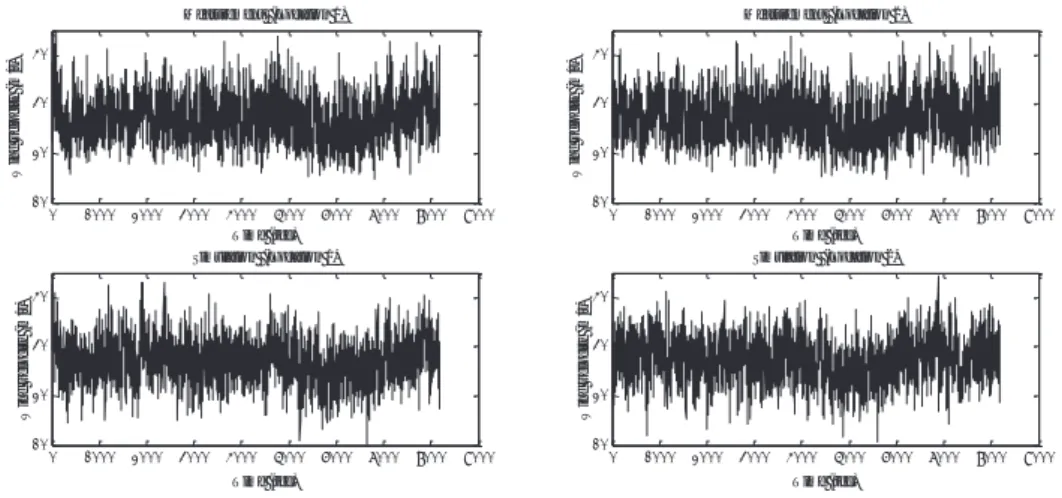
Figure 7The measurements and simulation results of multivariate wind processes.

Figure 8Coefficients of cross-correlation function.

4 CONCLUSION

A methodology of simulating univariate and multivariate turbulence flows in wavelet domain is proposed. This method, utilizing the Log-Poisson random cascade model, emphasizes the inter-nal intermittency effect of the turbulence fluctuations in this simulation. The simulation results agree with both the power spectrum and the statistical information presented by the scaling law, thus present a better representation of the natural wind process than the conventional methods which only considers the second-order moments. Furthermore, in the simulation of the multivari-ate processes, the wavelet coefficients are iteratively updmultivari-ated to match the wavelet coefficients coherence at the same scale, thereby guaranteeing the consistence of the cross correlation func-tion between the measurement and the simulafunc-tion results.

0 1000 2000 3000 4000 5000 6000 7000 8000 9000 10 20 30 40 T ime (sec) W in d v elo city ( m /s ) Measurement (Location 1) 0 1000 2000 3000 4000 5000 6000 7000 8000 9000 10 20 30 40 T ime (sec) W in d v elo city ( m /s ) Measurement (Location 2) 0 1000 2000 3000 4000 5000 6000 7000 8000 9000 10 20 30 40 T ime (sec) W in d v elo city ( m /s ) Simulation (Location 1) 0 1000 2000 3000 4000 5000 6000 7000 8000 9000 10 20 30 40 T ime (sec) W in d v elo city ( m /s ) Simulation (Location 2) 0 100 200 300 400 500 600 5.5 5.6 5.7 5.8 5.9x 10 6

T ime Interval (sec)

C ro ss -co rr el at io n C o ef fi ci en t Measurement Simulation

The Seventh International Colloquium on Bluff Body Aerodynamics and Applications (BBAA7) Shanghai, China; September 2-6, 2012

5 ACKNOWLEDGEMENTS

The support for this project provided by the NSF Grant # CMMI 09-28282 which is gratefully acknowledged. We also thank Dr. Kurtis R. Gurley for the assistance in programming the multi-variate non-Gaussian simulation and providing the data set.

6 APPENDIX

A. When time interval is 1sec, the Fourier spectrum of Haar wavelet function is shown as

Figure 9 Absolute Fourier spectrum of Haar wavelet

B. The Discrete Haar wavelet reconstruction algorithm is shown as follows:

,

2 1 2 1 1 1 , ~ , 1, , 2 2 n j j i n j k j V k j n j l i k m b a Gv k u u

¦

(15)

In order to explain clearly the relation between velocity difference

j

l v

G and wavelet coeffi-cient m_V

b a_k, _j

, the above algorithm is expressed in unnormalized form. Specifically, suppose a wind process v t including 8 discrete points, there are

3,1 3,2 3,4 2 , 2 , 1, 1 3 1 2 2 3 3 4 4 3 7 8 2 4 1 2 1 3 2 4 2 2 5 7 6 8 1 3 4 1 1 1 5 2 6 3 7 4 8 1 , ~ , , ~ , , , ~ 1 1 1 1 , ~ , , ~ 2 2 2 2 1 1 , ~ 4 4 i i i V l V l V l V l V l i i V l i m b a v v v m b a v v v m b a v v v m b a v v v v v m b a v v v v v m b a v v v v v v v v v G G G G G G ª_¬ º_¼ ª_¬ º_¼ ª_¬ º_¼

¦

¦

¦

(16)

When applied in the reconstruction like the simulation in this study,

^ `

,

j i

l v

G represent a i.i.d sequence. Therefore, m b a

_k, _j

is another random variable different from

j

l v

G , furthermore, in-dicated by Central Limit Theorem, m b a

_k, _j

approaches Gaussian distribution closer than

j

l v

G .

C. The relation between the wavelet coefficients cross-correlation at the same scale and the con-ventional cross-correlation is shown as[11]

2 1 1 2 1 1 2 2 * 1 2 1 2 1 1 2 2 * * 1 1 1 2 2 2 1 2 1 2 * * 1 1 1 2 2 2 1 2 1 2 * 1 1 2 2 1 2 1 2 , , , , , , , , , 2 2 2 , X Y m m i t t f a a a it f a it f XY C b b a a m b a m b a t b a t b a x t y t dt dt t b a t b a x t y t dt dt t b e t b e R t t e dt dt \ \ \ \ \ \ f f f f f f f f f f f f f f

³

³ ³

³ ³

³ ³

(17) 0 0.5 1 1.5 2 2.5 3 x 10-3 0 0.2 0.4 0.6 0.8 1 Frequency f (Hz) 2 (j -1 )/ 2 \ j (f) j=1 j=2 j=3 f j=0.742x2 -(n-j )

f

³

Then it can derive the following expressions

2 , , 2 j X Y j a m m j a b XY C W a f\ f S f df f

³

(19)

,

2 , 2 j X Y j a m m j a b XY C f a \ f S f (20)

,

2 , 2 j V V j a m m j a b VV C W a f\ f S f df f

³

(21)

,

2 , 2 j V V j a m m j a b VV C f a \ f S f (22)

Obviously, a stationary process implies a scale-dependent stationary process.

7 REFERENCES

1 Gurley, K. and Kareem, A., Applications of Wavelet Transforms in Wind, Earthquake and Ocean Engineer-ing, Engineering Structures, 21(2) (1999): 149-167.

2 Kitagawa, T. and T. Nomura, A wavelet-based method to generate artificial wind fluctuation data, Journal of Wind Engineering and Industrial Aerodynamics, 91(7)(2003): 943-964.

3 She, Z.-S. and E. C. Waymire, Quantized Energy Cascade and Log-Poisson Statistics in Fully Developed Tur-bulence, Physical Review Letters, 74(2) (1995): 262-265.

4 R.G. Ghanem, P.D. Spanos, Stochastic finite elements: a spectral approach, Springer-Verlag, New York, 1991. 5 K.K. Phoon, H.W. Huang, et al., Comparison between Karhunen-Loeve and wavelet expansions for simulation

of Gaussian processes, Computers & Structures, 82(13-14) (2004): 985-991.

6 C.W. Van Atta and W.Y. Chen, Statistical self-similarity and inertial subrange turbulence, Statistical models and turbulence, Lecture Notes in Physics 12, edited by M. Rosenblatt and C.W. Van Atta, Springer-Verlag, Ber-lin, (1972), pp. 402-426.

7 Z.-S. She and S. A. Orszag, Physical model of intermittency in turbulence: Inertial-range non-Gaussian statis-tics, Physical Review Letters., 13(1991): 1701-1704.

8 Shinozuka, M. and G. Deodatis, Simulation of Stochastic Processes by Spectral Representation, Applied Me-chanics Reviews, 44(4) (1991): 191-204.

9 Gurley, K. R. and A. Kareem, A conditional simulation of non-normal velocity/pressure fields, Journal of Wind Engineering and Industrial Aerodynamics, 77±78 (1998): 39-51.

10 Gurley K. R., Modelling and simulation of non-Gaussian processes, PhD Thesis, University of Notre Dame, (1997).

11 =HOGLQ%$5HSUHVHQWDWLRQDQGV\QWKHVLVRIUDQGRP¿HOGV$50$*DOHUNLQDQGZDYHOHWSURFHGXUHV3K'