Edge-elements Formulation of 3D
CSEM in Geophysics: A Parallel
Approach
Octavio Castillo Reyes
Department of Computer Architecture
Polytechnic University of Catalonia
This dissertation is submitted for the degree of
Doctor of Philosophy in Computer Architecture
José María Cela Espín
Electromagnetic methods (EM) are an invaluable research tool in geophysics whose relevance has increased rapidly in recent years due to its wide industrial adoption. In particular, the forward modelling of three-dimensional marine controlled-source electromagnetics (3D CSEM FM) has become an important technique for reducing ambiguities in the interpretation of geophysical datasets through mapping conductivity variations in the subsurface. As a consequence, the 3D CSEM FM has real application in many areas such as hydrocarbon and mineral exploration, reservoir monitoring, CO2 storage characterization, geothermal reservoir imaging and many others due to there quantities often displaying conductivity contrasts with respect to their surrounding sediments. However, the 3D CSEM FM at real scale implies a numerical challenge that requires an important computational effort, often too high for modest multicore computing architectures, especially if it fuels an inversion process. In this regard, the 3D CSEM FM is a key application that can benefit strongly from algorithmic and computational improvements.
On the other hand, although the High-performance Computing (HPC) code devel-opment is dominated by compiled languages, the popularity of high-level languages for scientific computations has increased considerably. Among all of them, Python is probably the language that has shown more interest, mainly because of flexibility and its simple and clean syntax. However, its use for HPC geophysical applications is still limited, which suggests a path for research, development and improvement. Therefore, this thesis reports the attempts at designing and implementing a method-ology that has not been systematically applied for solving 3D CSEM FM with an HPC application baked upon Python. The net contribution of this effort is the devel-opment and documentation of a new open-source modelling code for 3D CSEM FM in geophysics, namely, the Parallel Edge-based Tool for Geophysical Electromagnetic Modelling (PETGEM). The importance of having this modelling tools lies in the fact
that they provide synthetic results that can be compared with real data which has a practical use both in the industry and academia. Still, available 3D CSEM FM codes are usually written in low-level languages (Fortran, C-like) whose implemented
methods are often innaccessible to the scientific community since they are commercial.
PETGEM is written mostly in Python and relies onmpi4pyandpetsc4py packages for parallel computations. Other scientific Python packages used include Numpy and Scipy. This code is designed to cope with the main challenges encountered within the numerical simulation of the problem under consideration: tackle realistic prob-lems with accuracy, efficiency and flexibility. It uses the Nédélec Edge Finite Element Method (EFEM) as discretisation technique because its divergence-free basis is very well suited for solving Maxwell’s equations. Furthermore, it supports completely un-structured tetrahedral meshes which allows the representation of complex geometries and local refinement, positively impacting the accuracy of the solution. The parallel implementation of the code using shared-memory and distributed-memory architec-tures is investigated and described throughout this document. In addition, an exten-sive analysis of the parallel performance factors has proved that PETGEM is highly
scalable (hundreds of CPUs) allowing simulation of large cases for 3D CSEM FM (tens of millions of degrees of freedom).
In addition, the thesis deals with the numerical and physical challenges of the 3D CSEM FM problem. Through this work, frequency-domain Maxwell’s equations have been discretised using EFEM and validated by comparison with analytical solutions and published data, proving that modelling results are highly accurate. Furthermore, this work discusses an automatic mesh adaptation strategy for a given frequency and a specific source position. The results show that adaptive mesh solutions have a factor of savings of up to four times in runtime solution compared to those computed without the use of the meshing technique. Moreover, a convergence study of the parallel Krylov subspace iterative solvers that are widely used in the literature for solving the EM problem is presented. Test results show that the GMRES method in combination with SOR is the best choice for the EM problem under consideration since it shows a better convergence rate and requires less computation time.
In summary, this thesis shows that it is possible to integrate Python with HPC for the solution of the 3D CSEM FM problem at large scale in an effective way. The resulting modelling tool is easy to use and extend and the adopted algorithms are not only accurate and efficient but also have the possibility to easily add or remove components without having to rewrite large sections of the code.
Keywords: 3D electromagnetic modelling, geophysics, Python, high-performance
to my sisters, Esmeralda and Atalia, to my beloved wife, Magaly Basurto López, and in memory of my grandmother. I love you all dearly.
Acknowledgements
I wish to express my sincere appreciation to those who have contributed to this thesis and supported me in one way or the other during this amazing journey.
I am deeply thankful to my advisor, José María Cela Espín for accepting me in his research team, the Computer Applications in Science & Engineering depart-ment (CASE)in theBarcelona Supercomputing Center-Centro Nacional de Supercom-putación (BSC-CNS). I am very grateful for his support, guidance, encouragements and for countless time-intensive discussions during my research work; for bringing me to the project I worked on and giving enough freedom to implement and test my ideas. My special and sincere gratitude goes out to my co-advisor, Josep de la Puente from the BSC-Repsol Research Center. He has provided crucial guidance and support at every moment during my research path. For comments and ideas that helped me to improve my papers as well as this thesis, and all discussions during which we were always on the same level and I never felt being rigorously supervised, but rather constructively guided. Through numerous research meetings with him, I learned not only geophysical-electromagnetic insights and wisdom but also how to communicate scientific ideas.
I express my thanks to all the people I had as friends and as colleagues from the BSC-Repsol Research Center: Mauricio Hanzich, Natalia Gutiérrez, Juan Esteban Rodríguez, Albert Farres, Otilio Rojas, Samuel Rodríguez and Miguel Ferrer. I express my special thanks to David Modesto for proofreading my dissertation and papers, and for his constructive remarks and invaluable discussions in which he genuinely shared he knowledge, for all questions he patiently answered. In the same way, I am deeply grateful to Claudia Rosas for her time and advice in the incredible world of methodologies for scalability prediction and the analysis of fundamental performance factors for HPC applications.
I am grateful to all of my colleagues fromCASE of BSC-CNS. I am deeply thank-ful to Mariano Vásquez for his invaluable comments and constructive criticism that absolutely improved this manuscript. A deep thanks to Xevi Roca, Abel Gargallo and Miguel Zavala for all the fruitful discussions on numerical modelling, finite elements
I wish also to thank all members of BSC-CNS. Above all, I want to thank Mateo Valero for his support and encouragement. His vision for an excellent and relevant science is reflected in every corridor of the BSC-CNS. For me, it has been an honor to be part of this research center that is full of interesting people who constitute a warm and welcoming environment for the development of quality science and research. Thanks for opening the doors ofBSC-CNS and for showing me the extraordinary and magnificient supercomputing architecture that prides Spain: Marenostrum. I would also like to express my gratitude to Ulises Cortés for his advice and for the experiences organizing the Jornadas de Cooperación CONACyT-Catalunya. At the same time, I am greatly indebted to the Administrative Staff and Support Team of the BSC-CNS for all their management and technical support to carry out my research.
Beyond the borders of the BSC-CNS, several other people also deserve my thanks for their help. In November 2015 and March 2017, I visited theMaguique 3D research group at the National Institute for Computer Science and Applied Mathematics (IN-RIA) in Pau, France. I am extremely grateful to Hélène Barucq, Julien Diaz and Victor Péron for many useful discussions about the core of my research work and their hospitality during my visits. Thank you for your invaluable comments and for sharing your knowledge of geophysical electromagnetic modelling. In October-December 2016 I visited thePretroleum and Geosystems Engineering research group at theUniversity of Texas (UT)in Austin, USA. I am thankful to the Prof. Carlos Torres-Verdin for his willingness to be my host and for helping me to improve my work by sharing his broad experience with kindness. During my stay at UT I was able to learn about modelling tools in industry and some advanced programming practices which are carried out in one of the most powerful supercomputers in the world: Stampede. Also, I would like to express deep gratitude to Prof. Yonghyun Chung from Seoul National University (SNU) in South Korea, for his kindness and hospitality during my visit in July 2016. Our flash meetings enriched not only my research work but also my knowledge about the exciting Korean culture.
I would also like to thank colleagues and friends in my beloved Mexico, mainly those from Universidad Veracruzana. First, none of this would have happened without the support of Dr. Mario Miguel Ojeda, who believed in me enough to offer me my first laboral opportunity and, some years after, for give me his recommendation which opened me a scientific world with endless opportunities. I am very grateful for his guidance, encouragements and for countless discussions about my PhD project and my academic carrer. I wish also to thank Dr. Carlos Manuel Welsh Rodríguez for
sharing his scientific vision with me and for provided me a good platform to present and openly discuss ongoing work. I also thank to MSc. Rubén González Benítez for his support, advice and friendship that has lasted since he directed my master’s thesis. My gratitude extends to other academic and research institutes in Mexico for their kindness and hospitability: Centro de Investigación en Computación-(CIC-IPN) and Centro de Investigación y de Estudios Avanzados-(CINVESTAV-IPN).
I would like to express my sincere gratitude to the Mexican National Council for Science and Technology (CONACyT) for the financial support to develop my thesis. I am convinced of the value of the CONACyT scholarship program and although investment in science remains a long and difficult route, the progress is irreversible. I wish also thanks to the European Union’s Horizon 2020 research and innovation programme for his financial support under Marie Sklodowska-Curie grant agreement No. 644202 which allowed me to carry out 3 research stays that improved my work and my scientific background.
I am indebted to all my friends in Barcelona who opened their homes to me during my time at BSC-CNS and who were always so helpful in numerous ways. Special thanks to Benítez Domínguez family: Luisa, Fernando, Gemma, Alba, Sira and Leo. Thank you for your hospitality and for sharing wonderful and unforgettable moments, as well as for the long and interesting conversations that extended my vision and knowledge about Spanish culture. Their friendship is one of my greatest non-academic achievements of which I am proud.
I would like to express my love and gratitude to one of the dearest hopes of my life, my parents, Sergio Castillo and Antonia Reyes Banda. I will never forget your gestures of protection, of affection and of indulgence, all of them will remain sculpted in my heart forever. You have forged my soul with discretion under the magnifying glass of your example and the little that is good in me, carries your emblem. I always thank to my sisters Esmeralda and Atalia for his emotional support and for taking care of my parents during my long absence, as well as for always following me with your thoughts and for sharing my dreams. I am deeply thankful to my uncle Mauricio Reyes Banda for his support and for his continuous calls that kept us close despite the physical distance between us. I also express my deep gratitude to my parents-in-law for their support and prayer for my wife Magaly Basurto López and me.
Finally, my gratitude goes to Maggie, who has been by my side throughout this PhD, living every minute of it, and without whom, I would not have had the courage to carry it to a successful conclusion. She had faith in me and my intellect even when I felt like digging hole and crawling into one because I did not have faith in
inexhaustible source of joy and strength, as well as being a compass that helped me to reorganize my priorities and efforts. I think we have learned a lot about life and this stage strengthened our commitment and determination to live to the fullest. Thank you Maggie for sharing with me your happiness for life, thank you for exploring the city and the world at my side, as well as for our long and interesting conversations on topics beyond computer architecture and science. I have always felt happy to share my life with you.
Contents
List of figures xi
List of tables xiii
1 Introduction 1
1.1 3D CSEM FM in geophysics . . . 3
1.2 Present modelling challenges of 3D CSEM FM . . . 5
1.2.1 Discretisation remarks . . . 6
1.2.2 Computational remarks . . . 8
1.3 Summary and thesis objectives . . . 10
2 HPC python code for 3D CSEM FM 12 2.1 EFEM formulation for 3D CSEM FM . . . 14
2.2 Field interpolation with EFEM . . . 18
2.3 Algorithms for EFEM . . . 18
2.4 PETGEM . . . 25
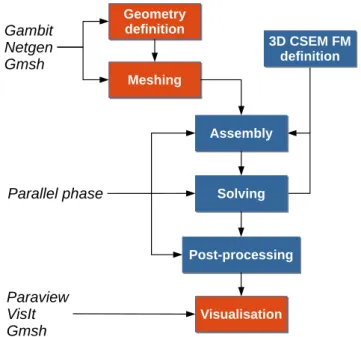
2.4.1 Code workflow . . . 26
2.4.2 Software stack overview . . . 27
2.4.3 Programming language . . . 29 2.4.4 Target architectures . . . 30 2.4.5 Requeriments . . . 30 2.4.6 Coding style . . . 31 2.4.7 Python 3.x compatibility . . . 31 2.4.8 Code availability . . . 32 2.5 Parallel strategies . . . 32
2.5.1 Parallelism on shared-memory platforms . . . 33
2.5.2 Parallelism on distributed-memory platforms . . . 34
2.6.1 Shared-memory tests . . . 38
2.6.2 Distributed-memory tests . . . 40
3 Use cases of 3D CSEM FM 44 3.1 Canonical model of an off-shore hydrocarbon reservoir . . . 44
3.2 3D CSEM FM with bathymetry . . . 48
3.3 Synthetic model with real target . . . 50
3.4 Automatic mesh adaptation . . . 58
3.5 Convergence of solvers . . . 61
4 Conclusions and future work 70 4.1 Conclusions . . . 70
4.2 Future directions . . . 73
5 Papers from the thesis 76 References 81 Appendix A Maxwell’s equations theory 91 Appendix B Numerical techniques in electromagnetics 95 B.1 Finite Element Method (FEM) . . . 96
B.2 Edge Finite Element Method (EFEM) . . . 114
B.3 Test case of EFEM . . . 125
Appendix C Prototyping and validation with synthetic test 129 C.1 Prototype for 3D CSEM modelling . . . 129
C.1.1 Synthetic test for mass matrix . . . 130
C.1.2 Synthetic test for stiffness matrix . . . 131
List of figures
1.1 Marine CSEM . . . 5
2.1 Global/local edge direction . . . 23
2.2 PETGEM workflow . . . 28
2.3 PETGEM software stack . . . 28
2.4 Array population for global system on shared-memory architectures . . 34
2.5 Parallel assembly on shared-memory architectures . . . 35
2.6 Parallel assembly on distributed-memory architectures . . . 36
2.7 Scalability tests on shared-memory architectures . . . 39
2.8 Scalability tests on distributed-memory architectures . . . 40
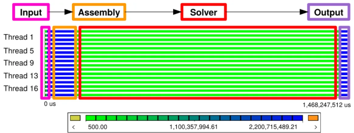
2.9 Main computational phases in PETGEM . . . 42
2.10 Scalability ratio of main computational phases in PETGEM . . . 42
2.11 Solver scalability analysis using Paraver . . . 43
3.1 Model 1 description . . . 45
3.2 Amplitude and phase analysis of model 1 . . . 46
3.3 Relative errors analysis of model 1 . . . 47
3.4 Convergence analysis of model 1 . . . 47
3.5 Model 2 description . . . 49
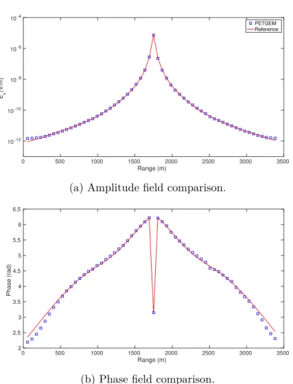
3.6 Amplitude and phase analysis of model 2 . . . 51
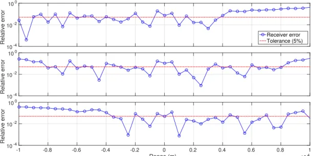
3.7 Relative errors analysis of model 2 . . . 52
3.8 Model 3 description . . . 53
3.9 Amplitude analysis of model 3 . . . 54
3.10 Phase analysis of model 3 . . . 55
3.11 Relative amplitude errors of model 3 . . . 56
3.12 Relative phase errors model 3 . . . 57
3.13 Amplitude analysis of model 4 . . . 62
3.15 Relative amplitude errors of model 4 . . . 64
3.16 Relative phase errors model 4 . . . 65
3.17 Times comparison between adapted and oversampled meshes . . . 66
3.18 Convergence rate of GMRES and BiCGSTAB solvers . . . 69
B.1 Discretisation in 2D . . . 103
B.2 Tetrahedral nodal element . . . 109
B.3 Triangular edge element . . . 116
B.4 Vector basis functions for triangular edge element . . . 118
B.5 Tangential/normal components for triangular edge element . . . 119
B.6 Tetrahedral edge element . . . 121
B.7 Convergence analysis of edge elements for 2D eddy-current problem . . 127
B.8 Solution of eddy-current problem in 2D . . . 128
C.1 Matlab prototype for 3D CSEM FM . . . 130
C.2 Mass matrix analysis . . . 132
C.3 Mass matrix convergence analysis . . . 133
C.4 Stiffness matrix analysis . . . 138
List of tables
2.1 Data structures for nodal elements . . . 18
2.2 Data structures for edge elements . . . 19
2.3 Matrix connectivity in 2D . . . 19
2.4 Edges computation and sorting . . . 21
2.5 Edge to node/element connectivity - first approach . . . 22
2.6 Element to edges connectivity in 2D - first approach . . . 22
2.7 Node to elements connectivity in 2D - first approach . . . 23
2.8 Element to edges connectivity in 2D - second approach . . . 23
2.9 Edge to node/element connectivity - second approach . . . 24
2.10 Nodal connectivity for local/global edge direction . . . 25
2.11 Elements to edges connectivity for local/global edge direction . . . 25
2.12 Elements to edges connectivity for local/global edge direction . . . 25
2.13 Execution results on shared-memory architectures . . . 39
2.14 Execution results on distributed-memory architectures . . . 41
3.1 Summary of convergence results for model 1 . . . 48
3.2 Mesh information based on automatic mesh adaptation . . . 60
3.3 Summary of results for automatic mesh adaptation tests . . . 61
3.4 Mesh information for solver convergence tests . . . 67
3.5 Summary of runtime for solver convergence tests . . . 68
B.1 Element to nodes connectivity in 2D . . . 102
B.2 Edge definition for triangular element . . . 116
B.3 Edge definition for tetrahedral element . . . 122
B.4 Summary results for 2D eddy-current problem . . . 127
C.1 Levels of mesh refinement . . . 134
C.2 Summary of errors for mass matrix tests . . . 135
C.4 Summary of errors for stifness matrix tests . . . 137 C.5 Summary of convergence rate for stiffness matrix tests . . . 137
Chapter 1
Introduction
The science of exploration geophysics applies the principles of physics to study the Earth. Geophysical surveys of the interior of the Earth involve taking measurements at or near the Earth’s surface that are influenced by the internal distribution of physical properties. Analysis of these measurements can reveal how the physical properties of the Earth’s interior vary vertically and laterally. By working at different scales, geophysical prospecting (GP) methods may be applied to a wide range of investigations from studies of the entire Earth (Kearey et al., 1996) to exploration of a localized region of the upper crust for engineering or other purposes of great societal value such as environmental surveys (e.g. Gibson et al., 1996; Marchetti et al., 2002; Gajewski et al., 2005), water prospecting (e.g. Perttu and Wikberg, 2005), geothermal energy applications (e.g. Koon and Ufondu, 2015) and oil & gas sector (e.g. Davydycheva et al., 2003; Strack and Aziz, 2012; Puzyrev et al., 2013; Chung et al., 2014).
An alternative method of investigating subsurface geology is, of course, by drilling boreholes, but these techniques are invasive and expensive and provide information only at discrete locations. GP, although sometimes prone to major ambiguities or uncertainties of interpretation, provides a relatively rapid and cost-effective means of deriving a really distributed information on subsurface geology. In the exploration for subsurface resources the methods are capable of detecting and delineating local features of potential interest that could not be discovered by any realistic drilling technique. Geophysical surveying does not dispense with the need for drilling but, properly applied, it can optimize exploration surveys by maximizing the rate of ground coverage and minimizing the drilling requirement.
Regardless of the scope or scale of the surveys, exploration geophysics methods are based on studying the propagation of the different physical fields within the Earth. In the context of geophysical exploration, the main target of these methods is to
build a constrained model of geology, lithology and fluid properties based upon which commercial decisions about reservoir exploration, development and management can be made (Koldan,2013). Nowadays, the three main technologies in applied geophysics are: seismic methods, potential field methods (magnetic and gravity approaches) and electromagnetic methods. Each of these methods processes a set of data within an integrated framework, so that the resultant Earth model is coherent with all data used in its construction.
In the oil & gas sector, the seismic methods have become a standard technique for obtaining high-resolution images of structure and stratigraphy of the Earth. However, seismic data have extremely poor sensitivity to changes in the type of fluids, such as water, brine, oil & gas. It is the main reason why in some scenarios it is difficult, if not impossible, to determine fluid properties from seismic data. The drawback of the seismic method of determining the presence of oil in a formation, encouraged the development of new methods aimed to strengthen the models and reduce uncertainty. In this sense, the electromagnetic methods (EM) have received special attention from industry and academia.
On top of that, the last decade has been a period of rapid growth for EM in geophysics, mostly because of their industrial adoption. In particular, the 3D ma-rine controlled-source electromagnetic (3D CSEM) method has become an important technique for reducing ambiguities in data interpretation in hydrocarbon exploration. Furthermore, in order to be able to predict the EM signature of a given geological structure, modelling tools provide us with synthetic results which we can then com-pare to real data. In particular, if the geology is structurally complex, one might need to use methods able to cope with such complexity in a natural way by means of, e.g., an unstructured mesh representing its geometry. Among the modelling methods for EM based upon 3D unstructured meshes, the Nédélec Edge Finite Element Method (EFEM) offers a good trade-off between accuracy and number of degrees of freedom (DOFs), i.e. size of the problem. Furthermore, its divergence-free basis is very well suited for solving Maxwell’s equations.
This thesis provides the numerical formulation of EFEM 3D CSEM forward mod-elling (FM) in geophysics and its implementation on massivelly parallel computers using an interpreted language, namely, Python. It enables the possibility to specify edge-based variational forms ofH(curl) for the simulation of electromagnetic fields in
real 3D CSEM FM surveys with high flexibility accuracy. The new modelling tool is based on two main contributions controlling the structure of the document: firstly, the integration of EFEM and cutting-edge High-performance Computing (HPC)
technolo-1.1 3D CSEM FM in geophysics
gies for efficient 3D CSEM FM. Secondly, the study of the scopes of the computational tool through real-scale modelling. Its solution is evaluated by comparison to well-established 3D CSEM models. The flexibility, accuracy and modularity of the code makes it a competitive tool to simulate real scenarios of 3D CSEM FM in geophysics. The purpose of this Chapter is to give a brief review of the 3D CSEM FM in exploration geophysics. Next, thesis contributions are introduced with emphasis on state-of-art modelling challenges. Finally, the thesis objectives are presented.
1.1
3D CSEM FM in geophysics
EM are an established tool in geophysics, with application in many areas such as hydrocarbon and mineral exploration, reservoir monitoring, CO2 storage characteriza-tion, geothermal reservoir imaging and many others. Presumably the most successful application for oil prospecting has being well logging which was introduced by the Schlumberger brothers (Johnson,1962). Jishan and Lizhi (1999), Tang et al.(2007),
Xue et al. (2008) and Constable (2010) summarized and reviewed the development of EM survey techniques in terms of instrument, acquisition, processing and interpre-tation, numerical simulation, and application respectively.
For the diversity of remote sensing techniques that were deployed in the past century, EM seem to be of less importance compared to seismic techniques in the oil & gas sector. However, the activity in EM for exploration has not been absent, and in the 1970’s and 1980’s, improved equipment and increasing data-processing power led to extensive development. Nowadays, EM is a fundamental tool in the oil & gas industry because of the hope that the application of such methods would eventually lead to the direct detection of hydrocarbons through their insulating properties.
The electromagnetic properties of a medium are described by three elements: the electric permittivity or dielectric constantϵr(F m−1), magnetic permeabilityµ(Hm−1)
and electric conductivityσ(Sm−1) or its reciprocal called electric resistivity 1/σ(Ωm). Since the Earth is conductive, the attenuation of propagating waves becomes more se-vere as the signal frequency increases (Løseth,2007). Hence, the aim of the most EM in geophysics is to measure the resistivity of the Earth materials. A strong description of the different methods of resistivity measurement and different possibilities to vary the source type (e.g. electric or magnetic dipole) and source signal (e.g. time-harmonic, direct current, or transient) can be found in (Nabighian, 1988).
Since the electric conductivity measure in a region could describe the properties and distribution of fluids in this area, EM for prospecting have become a standard
technique in oil & gas industry for mapping variations in the subsurface. In ( Ei-desmo et al., 2002; Edwards, 2005; Sheard et al., 2005; Srnka et al., 2006; Newman and Commer, 2009; Gray et al., 2012; Chung et al., 2014; Cai et al., 2017) can be found several examples which establish that the electrical conductivity of petroleum, gas or hydrate bearing sediments is based on the concept of an increased resistivity in hydrocarbon-rich zones. Because the ability to map significant contrast between electric conductivity, EM are very useful for detecting hydrocarbon locations.
3D CSEM FM techniques, also referred as seabed logging or marine 3D CSEM ( Ei-desmo et al.,2002), can be divided into two groups depending on the domain in which collected data is interpreted: time domain (TDEM) or frequency domain (FDEM). This thesis focuses in FDEM theory. In 3D CSEM FM, a deep-towed electric dipole transmitter is used to produce a low frequency electromagnetic signal (primary field) which interacts with the electrically conductive Earth and induces eddy currents that become sources of a new electromagnetic signal (secondary field). The two fields, the primary and the secondary one, add up to a resultant field, which is measured by remote receivers placed on the seabed. Since the electromagnetic field at low frequen-cies, for which displacement currents are negligible, depends mainly on the electric conductivity distribution of the ground, it is possible to detect thin resistive layers beneath the seabed by studying the received signal (Koldan, 2013). Operating fre-quencies of transmitters in 3D CSEM FM may range between 0.1 and 10 Hz, and the choice depends on the dimensions of a model. In most studies, typical frequencies vary from 0.25 to 3 Hz, which means that for source-receiver offsets of 10-12km, the
pene-tration depth of the method can extend to several kilometres below the seabed (Hanif et al., 2011; Koldan, 2013). The main disadvantage of 3D CSEM FM is its relatively low resolution compared to seismic imaging. Therefore, 3D CSEM FM is often used in conjunction with seismic surveying as the latter helps to constrain the resistivity model. Figure 1.1 depicts the marine CSEM. Although 3D CSEM FM is nowadays a well-known geophysical prospecting tool and his fundamental mathematical theory is well-established, the state-of-art shows a relative scarsity of robust, flexible, modular and open-source codes to simulate these problems on HPC platforms, which is crucial in the future goal of solving inverse problems. In this regard some examples of mod-elling tools for geophysical prospecting are (Mackie et al., 1994; Alumbaugh et al.,
1996; Xiong et al., 2000; Zyserman and Santos, 2000; Badea et al., 2001; MacGregor et al., 2001; Fomenko and Mogi, 2002; Newman and Alumbaugh, 2002; Davydycheva et al., 2003; Key and Weiss,2006;Franke et al., 2007; Kong et al., 2007; Li and Key,
1.2 Present modelling challenges of 3D CSEM FM
Fig. 1.1 Marine CSEM.
2011; Li and Dai, 2011; Puzyrev et al., 2013;Koldan, 2013). However, the tools that full fit needs for the solution of real models are commercial and often are inaccessi-ble to the wider scientific community. Furthermore, due to the discretization method employed, not all codes that are affordable to community are capable of dealing with complex geometries and non-uniform bathymetries, which reduces or limits his use in situations which irregular and complicated geology has a significant influence on measurements. Additionally there are few parallel codes that are efficient, scalable and can deliver good performance.
This thesis proposes the development and documentation of a new parallel python code that meet the requirements of 3D CSEM FM at real-scale, namely, Parallel Edge-based Tool for Geophysical Electromagnetic Modelling (PETGEM). It has been
designed to cope with the various situations encountered within the numerical simu-lation of the 3D CSEM FM in geophysics. The code is based on the EFEM and pure Python language that allow users an easy adaptation to various 3D CSEM models and their fast execution on HPC arquitectures.
1.2
Present modelling challenges of 3D CSEM FM
3D CSEM FM maps resistive bodies such as carbonates, hydrocarbon filled sediments, volcanic rocks and salt from the seabed. Particularly in offshore hydrocarbon explo-ration, data regarding resistivity mappings beneath the seafloor is crucial and useful, namely, high resistivity of hydrocarbon filled rocks (30-500 Ωm) compared to bodies
filled with saline formation water (0.5-2 Ωm) is usually a good indicator for the
pres-ence of oil & gas (Constable and Weiss,2006;Constable and Srnka,2007;Key,2009). Because its capacity to detect, identify and characterize the target reservoir, the 3D CSEM modelling is an attractive and convincing method to conduct exploration
cam-paigns, thus increasing the drilling success rate as well as reducing associated cost and hazards.
The numerical properties of 3D CSEM FM algorithms in hydrocarbon exploration should be particularly sought for:
1. Accuracy. It is always desirable to obtain a numerical solution as accurate as
possible, although the uncertainties associated with the domain discretisation, numerical operator and the spatial singularity at the source (electric dipole). This leads to the need for a method that offers a good trade-off between accuracy and number of degrees of freedom (DOFs), namely, the key issue is to design an algorithm whose accuracy is determined by the control of those uncertainties.
2. Tackle realistic problems with efficiency. Due to the tremendous progress
of scientific computing geophysical imaging tackles more and more realistic mod-els. However, not all numerical schemes are well suited for latest computing architectures or are well adapted to the problem. Furthermore, the actual ex-ecution of real-life scale models requires the use of HPC resources. For that reason, an architecture-aware design effort is often beneficial in order to ensure that a new method has capacity for large scale computations, thus competence to deal with real models.
3. Adaptability, modularity and flexibility. The adopted algorithms should
cope with a variety of characteristic of the models with the possibility to easily add or remove components. The method should also run efficiently on a large variety of computer platforms without having to rewrite large parts of the code. It is also desirable to let to the user a minimum of parameters to tune. This can be satisfied with a correct use of third-party libraries which are usually optimized for the computer architecture being used.
This thesis proposes the use of state-of-art EFEM and cutting-edge HPC technologies to improve simultaneously the three key requirements already mentioned at real-scales.
1.2.1
Discretisation remarks
As principal discretisation techniques for 3D CSEM FM arises the Finite Difference Method (FDM), Finite Element Method (FEM) and Edge Finite Element Method (EFEM). The FDM, despite the disadvantage of not being able to precisely take into account complex geometries of subsurface structures, which in some cases may
1.2 Present modelling challenges of 3D CSEM FM
significantly damage the quality of a solution, is still the most widely employed dis-cretisation scheme (Koldan,2013). There are many successful FDM implementations, but the most practical and highly efficient parallel code was developed by (Alumbaugh et al., 1996). However, the main disadvantage of FDM is his incapacity to work with unstructured grids. An example of later issue is an scenario with seabed bathymetry where an imprecise representation produces artefacts in images that can lead to false interpretations (Koldan, 2013). On the other hand, FEM supports completely un-structured meshes as well as mesh refinement, which enables the representation of complex geometries and thus improve the solution accuracy. Despite, FEM is still not as widely applied as FDM and a major obstacle for its broader adoption is that the nodal FEM does not correctly take into account all the physical aspects of the vector field functions. In fact, there are three main problems when nodal-based fi-nite elements, obtained by interpolating the nodal values, are employed to represent vector fields (electric or magnetic). The first one is the occurrence of spurious solu-tions or non-physical solusolu-tions, which is generally attributed to lack of enforcement of the divergence condition. The second one is the inconvenience of imposing bound-ary conditions at material interfaces as well as at conducting surfaces. Finally, the third problem is the difficulty in treating conducting and dielectric edges and corners due to field singularities associated with these structures. Consequently, most of the researchers who have employed the FEM for 3D CSEM FM have been primarily fo-cused on overcoming this problem, as well as on solving other physical and numerical challenges, in order to obtain a proper and accurate numerical solution, leaving aside the performance of the codes (Koldan, 2013). These drawbacks have encouraged the exploration of other approaches, namely, EFEM. This technique uses so-called vector basis functions that assign DOFs to the edges rather than to the nodes of each element.
This thesis focuses on EFEM as discretisation approach because it is based on unstructured meshes, which offer more convenient mesh adaptivity (refinement) and better fit to complex domains. Furthermore, the use of this meshes is more suitable because they allows place more grid points in areas where the solution error is large, avoiding the necessity to create a fine mesh over the whole domain. Examples of geophysical applications with FEM and EFEM can be found in (Ho-Le, 1988; Badea et al., 2001; Bespalov et al., 2007; Hanif et al., 2011; Koldan, 2013; Puzyrev et al.,
1.2.2
Computational remarks
The EFEM computational implementation is very similar to that which uses usual node-based elements. However, the main difference arises in the preparation of the input data. Since in EFEM the unknowns are associated with the edges of elements, new data structures are requiered, namely:
1. Elements connectivity matrix defined by their 3/6 in 2D/3D. 2. Edges matrix defined by their 2 nodes in 2D/3D.
3. Numbering strategy to ensure the tangential continuity of edges.
Since most of the FEM codes were developed for node-based finite elements, it is necessary to develop a small library to build up the previous data structures. Many strategies have been discussed in depth (Owen,1998;Said et al.,1999;Chrisochoides,
2006; Zhang et al., 2008; Jamin et al., 2014; Knepley et al., 2015). However these approaches can be very time-consuming for meshes with a considerable number of elements, which is a normal requirement in real scenarios of 3D CSEM FM. Therefore, Chapter 2 of this thesis presents a new set of algorithms for EFEM computations.
Because of the extremely heavy 3D CSEM FM requeriments at real-scale, re-searchers aim at highly optimized implementations running on HPC architectures. Normally, this demands a need for developing tailored, hand-tuned codes in compiled languages: C-like and Fortran. However, there are not openly available and easily accesible ad-hoc codes to the public and the common geophysics researcher, e.g. the design is no user-friendly, and it is both challenging and time-consuming for a user to modify or extend the codes to satisfy their own needs. Latter issue is usually nature of codes written in low-level programming languages (compiled languages).
Over the last two decades the researchers have tended to move from low-level to high-level programming languages like Python, Matlab, R and Julia, among others. The experience is that implementations based on interpreted languages are faster to develop, easier to test and mantain, hardware-independent, and they can reach a much wider audience because the codes are readable and compact. The drawback of interpreted languages has been the decreased computational performance and, in particular, their lack of an efficient support for HPC architectures. However, a lot of progress has been made in theory as well as practice in order to reduce the cost of accessing to parallel environments through interpreted languages. From the long list of this kind of languages, Python is the option that has gained most popularity in the
1.2 Present modelling challenges of 3D CSEM FM
parallel scientific computing context. In fact, there are already several examples of succesfull use of Python for HPC applications:
1. FEniCS(Alnæs et al.,2015). Computational tool for solving partial differential
equations written mainly in C++, but most application developers are writting directly in Python. For large scale applications the developed Python solvers are usually equally fast as their C++ counterparts, because most of the computing time is spent within the low-level wrapped C++ functions that perform the costly linear algebra operation (Mortensen and Langtangen,2016).
2. Petsc4py (Dalcín et al., 2011). Open-source, public-domain software project
that provides access to the Portable, Extensible Toolkit for Scientific Compu-tation (PETSc (Balay et al., 2016)) libraries within the Python programming language. Petsc4py is a general-purpose and full-featured package. Its facilities allow sequential and parallel Python applications to exploit state-of-art algo-rithms and data structures readily available in PETSc.
3. Mpi4py (Dalcín et al., 2008). Open-source, public-domain software project
that provides bindings of the Message Passing Interface (MPI) standard for the Python programming language. Its facilities allow parallel Python programs to easily exploit multiple processors.
4. GPAW (Mortensen et al., 2005). Code devoted to electronic structure
calcula-tions, written as a combination of Python and C.
5. PyClaw (Ketcheson et al., 2012). Python-based interface to the algorithms of
Clawpack and SharpClaw for wave propagation problems. It also contains the PetClaw package, which adds parallelism through PETSc.
6. SfePy (Cimrman, 2014). Python code for solving systems of coupled partial
differential equations by the FEM in 1D, 2D and 3D. This code is useful for building custom applications.
7. pyGIMLi (Coscia et al., 2011). Open-source multi-method library for solving
inverse and forward tasks related to geophysical problems. Written in C++ and Python, it allow users build robust inversion applications in the geophysical context.
Python has potential for providing short and quick implementations to compete with tailored codes in low-level programming languages up to thousands of processors.
However, this fact is not well known in the geophysics context and the number of end-user parallel applications is still limited. Therefore, this thesis reports a novel HPC python implementation for 3D CSEM FM in geophysics aimed at a wide audience.
1.3
Summary and thesis objectives
The 3D CSEM FM is well established and widely used in industry and academy to define and characterize bodies by its electric resistivity, which help us to conduct exploration campaigns with a significant reduction of costs and risks (Osseyran and Giles, 2015). On the other hand, simulation and modelling tools help us to formalize and simplify the complexity we observe in nature. This simplification together to HPC advances allow us to render natural phenomena treatable and testable.
Although some contributions have been made to the development of algorithms and tools for 3D CSEM FM, such as parallel codes developed by (Alumbaugh et al.,
1996) and (Koldan,2013), the knowledge on this subject is still limited in the context of interpreted languages, with plenty of room for improvement. As main example, most codes that meet the requirements at real-scale modelling are based on compiled languages, are commercial and often inaccessible to the wider scientific community, aspects that can all hamper advancements in the field. Furthermore, these codes are not user-friendly which reduce the potential for a user to modify or extend them to satisfy their own needs. Therefore, this thesis is focused in the development of an approach that efficiently deals with this scenario.
The main goal is develop and document a new open-source modelling tool for 3D CSEM FM in geophysics using HPC architectures and Python as programming lan-guage, namely, Parallel Edge-based Tool for Geophysical Electromagnetic Modelling (PETGEM). This thesis considers Python as a glue language for interconnecting
differ-ent modules of codes written in compiled languages. By exploiting this methodology, complex scientific modelling codes can take advantage of the best attributes of both worlds: the efficient high-level data structures and a simple but effective approach to object-oriented programming of Python, and the well-know efficiency of compiled languages for numerically intensive computations. The code must tackle realistic prob-lems with accuracy, efficiency and flexibility. For this purpose, the following particular objectives are considered:
1. Efficient implementation of 3D CSEM FM on HPC. In literature few
related works can be found dealing with codes for the numerical solution of 3D CSEM FM using EFEM. Most of them are based on FEM or FDM and written
1.3 Summary and thesis objectives
with compiled languages, hence the use of interpreted languages in this context is a plenty room to investigate and improve. The first part of Chapter 2 is dedicated to the numerical formulation of EFEM for 3D CSEM FM and its implementation on state-of-art HPC architectures using Python programming techniques. A Matlab prototype for the solution of the problem under consideration is described in Appendix C. The algorithms developed seek to exploit the flexibility of the numerical method. Here, the HPC code is validated against the quasi analytical results of canonical models. In all cases the numerical solutions obtained were found in good agreement with reference models.
2. Performance evaluation of the code. Since some portions of the code are
interpreted and because there is some calling overhead for Python functions, the performance is traditionally deteriorated. The second part of Chapter 2 is devoted to the presentation of the code performance analysis. This is based on strong scalability studies and hardware counters analysis for the models of previous particular objective.
3. 3D CSEM FM at real-scale. An objetive of this thesis is the 3D CSEM FM at
real-life scale which requires the inclusion of real geometries, such as bathymetry, as well as a considerable number of DOFs. Since these models requires using HPC resources, an architecture-aware design effort is desirable in order to ensure that a new method has capacity for large scale computations. Chapter 3 presents a set of 3D CSEM FM models at real-scale. According to the results, flexibility, ease and accuracy of PETGEM makes it a competitive and attractive tool to
HPC python code for 3D CSEM
FM
Nowadays, the electromagnetic methods are an established tool in geophysics, with application in many areas such as hydrocarbon and mineral exploration, reservoir monitoring, CO2 storage characterization, geothermal reservoir imaging and many others. In particular, the 3D CSEM FM has become an important technique for reducing ambiguities in data interpretation for hydrocarbon exploration. In order to be able to predict the electromagnetic signature of a given geological structure, modelling tools provide us with synthetic results which we can then compare to real data. Additionally, in the multi-core and many-core era, parallelization is a crucial issue. Edge finite element method (EFEM) offer good scalability potential. Its low degrees of freedom (DOFs) number after primary/secondary field decomposition make them potentially fast, which is crucial in the future goal of solving inverse problems which might involve over 100,000 realizations (Osseyran and Giles, 2015).
As consequence, in past 2 decades the modelling tools have become one of the pil-lars for the simulation of numerical methods which main goal is elucidating the funda-mental mechanisms behind simplified abstractions of complex phenomena in different areas. The 3D CSEM FM in geophysics is no exception and the scientific community has developed important contributions in this field. In this regard some examples of modelling tools for geophysical prospecting are (Mackie et al.,1994;Alumbaugh et al.,
1996; Xiong et al., 2000; Zyserman and Santos, 2000; Badea et al., 2001; MacGregor et al., 2001; Dogru et al., 2002; Fomenko and Mogi, 2002; Newman and Alumbaugh,
2002; Collins et al.,2003; Davydycheva et al., 2003; Cao et al., 2005; Key and Weiss,
2006; Weiss and Constable, 2006; Franke et al., 2007; Kong et al., 2007; Li and Key,
and Rykhlinski, 2011; Li and Dai, 2011; Puzyrev et al., 2013; Koldan, 2013; Koldan et al., 2014). However, the tools that full fit needs for the solution of real models are commercial and often are inaccessible to the wider scientific community. Due to the discretization method employed, not all codes that are affordable to community are capable of dealing with complex geometries such as models including bathymetries. Additionally there are few parallel codes that are efficient, scalable and can deliver good performance.
On top of that, this thesis is focused in the development and documentation of a new open-source modelling code for 3D CSEM FM in geophysics using interpreted languages and its parallel and vectorized techniques on HPC platforms. An advantage of interpreted languages over compiled languages lies in the fact that it is much easier to make changes and test those modifications in a rapid way. On the other hand, the most mentioned disadvantage of interpreted languages, compared to compiled languages, is the performance (Dalcín et al.,2011). However, since computer hardware is increasing in speed rapidly, the language performance factor is less and less critical. Furthermore, for most scientific computing applications the time-critical portion of the code that requires the efficiency of a compiled language, is confined to small set of functions. Implementing the remaining part of the code using an interpreted language has many advantages without a considerable performance degradation.
Within the variety of interpreted languages, we have decided to use Python 3.x to develop a Parallel Edge-based Tool for Geophysical Electromagnetic Modelling ( PET-GEM). We chose Python 3.x language not only because is an highly flexible and open
source language but also because is the easiest and natural way to migrate the Matlab prototype that we developed in Appendix C. In addition, Python 3.x offers numerous third-party modules that make possible a rapid development.
Among others, PETGEM aims to solve a relative scarcity of robust edge-based
codes to simulate these problems on HPC architectures. PETGEM is implemented
in current state-of-art platforms such as Intel Xeon Platinum, Intel Haswell and In-tel Xeon Phi processors, which offer high-performance and flexibility. Nevertheless,
PETGEM support older architectures such as SandyBridge, for the sake of usability
and to be able to compare performance.
In this Chapter, the numerical formulation for the modelling of 3D CSEM using EFEM is presented. In addition, the algorithmic implementation and PETGEM
fea-tures are surveyed. Furthermore, parallel strategies in PETGEM are described in
depth. At the end of the Chapter we presented a PETGEM performance analysis on
2.1
EFEM formulation for 3D CSEM FM
Electromagnetic (EM) problems that arise in geophysics when using 3D CSEM FM generally deal with a resultant EM field wich appears as response of the electrically conductive Earth to an impressed (primary) field generated by a source (Koldan,2013). The primary field gives rise to a secondary field, and the resultant field is the sum of both fields.
3D CSEM FM involves the numerical solution of Maxwell’s equations in station-ary regimes for heterogeneous anisotropic electrically conductive domains in order to compute the components of the EM field. A broad description of these fundamental equations is included in Appendix A. 3D CSEM FM generally works with low fre-quency EM fields (0.1 Hz to 3 Hz) because the electric conductivity of the geological structures is much larger than their dielectric permittivity (Koldan, 2013). In conse-quence, Maxwell’s equations are simplify and reduce to their diffusive form (Zhdanov,
2009; Koldan, 2013; Cai et al.,2014)
∇×E=iωµ0H, (2.1)
∇×H=Js+ ˜σE, (2.2)
where we considered the harmonic time dependencee−iωt, ω is the angular frequency, µ0 is the free space magnetic permeability, Js is the distribution of source current, ˜σ
is the electric conductivity and E is the induced current in the conductive Earth. In
isotropic domains, ˜σ is an scalar value that is function of all three spatial coordinates.
On the other hand, in anisotropic domains, ˜σ is a 3×3 tensor defined as
˜ σ= σx 0 0 0 σy 0 0 0 σz , (2.3)
where σx,σy and σz are function of the spatial coordinates.
In 3D CSEM FM, the most used formulations for the field E are those based on
total field or primary/secondary field (electric field decomposition). In a total field formulation a slightly larger computational domain is required in order to discretize the source properly. Moreover, the rapid change of the primary current demands a dense mesh refinement near to the source. To overcome these difficulties, many authors use the primary/secondary field formulation, where the primary field corresponds to the solution in a layered earth. This formulation is desirable because the primary
2.1 EFEM formulation for 3D CSEM FM
field is much smoother than the source current, avoiding singularities near to the source and limiting the size of the computational domain. Therefore we have used a primary/secondary field approach.
Following the formulation by (Zhdanov, 2009; Cai et al., 2014), we decomposed the total electric field (Et) into primary field (Ep) and secondary field (Es) as
Et=Ep+Es, (2.4)
σ =σs+ ∆σ. (2.5)
Based on this decomposition, we derive the following expression for the secondary field
∇×∇×Es+iωµσEs=−iωµ∆σEp, (2.6)
where the source term is Ep. For a general layered earth model, Ep can be computed
semi-analytically by using Hankel transform filters. Therefore, the source term is given by a dipole able to work in each spatial coordinate (Nabighian, 1988), namely, a x-directed dipole is defined as
Ex = Υ· " d2x r2 # ·Ψ +k2r2−ikr−1, (2.7a) Ey = Υ· " dx·dy r2 # ·Ψ, (2.7b) Ez = Υ· " dx·dz r2 # ·Ψ, (2.7c)
a y-directed dipole is defined as
Ex = Υ· " dx·dy r2 # ·Ψ, (2.8a) Ey = Υ· " d2 y r2 # ·Ψ +k2r2−ikr−1, (2.8b) Ez = Υ· " dy ·dz r2 # ·Ψ, (2.8c)
and finally, a z-directed dipole is determined by Ex= Υ· " dx·dz r2 # ·Ψ, (2.9a) Ey = Υ· " dz·dy r2 # ·Ψ, (2.9b) Ez = Υ· " d2 z r2 # ·Ψ +k2r2 −ikr−1, (2.9c)
with Υ and Ψ defined as
Υ = 4I·dS
πσr3 ·e
−ikr
,
Ψ =−k2·r2+ 3ikr+ 3,
whereI is the dipole current, dS is the dipole length, σ is the background
conductiv-ity, k is the propagation parameter (wavenumber), r is the distance between source
position and the evaluation point position, and (dx, dy, dz) are the components of the
vector connecting source position and evaluation point position.
Equation (2.6) can be solved by using integral equation method (Chew et al.,2008;
Kythe and Puri,2011), FDM (Newman and Alumbaugh,2002;Newman et al.,2010), FEM (Key and Weiss,2006; Key and Ovall,2011) or EFEM (Cai et al., 2014;Chung et al., 2014; Cai et al., 2017). As already said, our formulation is based on EFEM which uses vector basis functions defined on the edges of the corresponding tetrahedral elements. Therefore, if the tangential components of the electric field E are assigned
to each edge, the components of E inside the tetrahedral elements can be expressed
as Exe = 6 X i=1 NxieExie, Eye= 6 X i=1 NyieEyie, Eze = 6 X i=1 NzieEzie, (2.10) where Ne
i are the vector edge basis functions defined by (Jin, 2002). Despite its
wide use, the literature about the computation of these basis is not easy to perveice. Therefore, in Appendix B.2 we included a detailed description in order to fill this relative scarcity. The compact form of these basis functions is defined as
Ee =
6
X i=1
NeiEei. (2.11)
2.1 EFEM formulation for 3D CSEM FM
element boundaries. Taking into account the EFEM background of Appendix B.2, and by substituting expression (2.11) into (2.6), and using Galerkin’s method, the weak form of the original differential equation is given by
Qi =
ˆ
Ω
Ni·[∇ × ∇ ×Es−iωµσE˜ s+iωµ∆˜σEp]dV. (2.12)
The discretized form of (2.12) for each tetrahedral element in the domain is obtained after applying the Green’s theorem
Qi =
ˆ
Ω
Ni·[∇ × ∇ ×Es−iωµσE˜ s+iωµ∆˜σEp]dV, (2.13)
where Ke and Me are the elemental stiffness and mass matrices defined as
Kije = ˚ Ve (∇×NeiSie)·(∇×NejSje)dV, (2.14) Mije = ˚ Ve( NeiSie)·(NejSje)dV, (2.15)
where Sie are coefficients equal 1 or−1 depending on the local and global direction of
thei-th edge in the element. Expression (2.13) can be written compactly as [A]· {ϕ}= {b}where matrix [A] is assembled from elemental matricesKe andMe, and similarly,
the vector {b}from elemental vectors {be}, namely
[Kjke +iωσ˜eMjke]· {Esk}=−iωµ∆˜σeRek, (2.16)
where Rek is the right hand side which requires numerical integration.
Proper boundary conditions need to be added in order to obtain a unique solution for system (2.16). For this purpose, we considered the homogeneous dirichlet bound-ary conditions in the EFEM formulation because these holds approximately for the secondary E at a distance from the domain with the anomalous conductivity (Jin, 2002)
e|∂Ω = 0. (2.17)
For the numerical simulation, the distance, where boundary conditions (2.17) hold, can be determined based on the skin depth of E. Fundamental references about that
2.2
Field interpolation with EFEM
To compute the Es in interested points, such as receivers position, is necessary to
perform an interpolation function. Based on the approach by (Jin, 2002; Zhdanov,
2009; Cai et al., 2014) and by using the vector basis functions (2.11), the Es for a
point r contained in element e, can be obtained by
Esr = ˆ
Nei ·Eesi·Sie i= 1. . .6, (2.18)
where Eesi is the secondary field assigned to the i-th edge of element e and Sie are
coefficients equal 1 or −1 depending on the relative local orientation of the i-th edge in the element e with respect to the global orientation of the i-th edge in the mesh, fully explained in Subsection 2.3 through expression (2.19).
2.3
Algorithms for EFEM
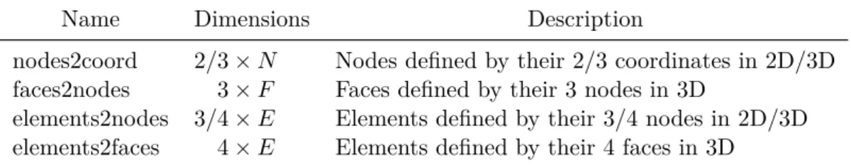
The implementation of a code based on EFEM is very similar to that which uses usual FEM. The main difference arises in the preparation of the input data, namely a nodal-based FEM standard code requires the data structures included in table 2.1, where N, E and F are the number of nodes, elements and faces respectively. Since
Name Dimensions Description
nodes2coord 2/3×N Nodes defined by their 2/3 coordinates in 2D/3D faces2nodes 3×F Faces defined by their 3 nodes in 3D
elements2nodes 3/4×E Elements defined by their 3/4 nodes in 2D/3D elements2faces 4×E Elements defined by their 4 faces in 3D
Table 2.1Main FEM data structures for linear triangular/tetrahedral nodal elements.
for the EFEM, the unknowns are associated to element edges, instead of the nodes, one needs a matrix to represent every element by their edges and another matrix to describe every edge by their two nodes, as show table 2.2 where E is the number of
edges. Because most of the FEM codes were developed for nodal-based FEM, it is necessary to develop a set of algorithms to build up the data structures of table 2.2, namely, convert node numbering into edge numbering. Traditional approach consists in go through element by element to check if all the edges of the i-th element have been numbered. If an edge has not been numbered, number it; otherwise, skip it (Jin,
2.3 Algorithms for EFEM
Name Dimensions Description
elems2edges 3/6×E Elements defined by their 3/6 edges in 2D/3D edges2nodes 2× E Edges defined by their 2 nodes in 2D/3D
Table 2.2 Main EFEM data structures.
2002). However, former technique can be very time-consuming for meshes with a considerable number of elements, which is a normal feature in real applications not just in the geophysics field, but also in others fields.
Many edge numbering strategies have been discussed in depth (Owen, 1998; Said et al.,1999;Chrisochoides,2006;Zhang et al.,2008;Jamin et al.,2014;Knepley et al.,
2015). This thesis focuses on the use and improvement of two of the most common techniques. In sake of simplicity, both algorithms are applied to a FE mesh in 2D which connectivity is presented in table 2.3. The first strategy start with the computation
e nodes(1,e) nodes(2,e) nodes(3,e)
1 2 4 1 2 2 4 5 3 2 3 5 4 3 5 6 5 4 5 7 6 5 7 8 7 5 6 8 8 6 9 8
Table 2.3 Element to nodes connectivity array in 2D.
of an edge id, which is given by simple operations such as (i1×i2), (i1/i2 +i2/i1) or (i1logi2+i2logi1), where i1 and i2 are the end-points of j-th edge. Its operation is applied to all elements in a nodal-based FE connectivity to list all edges in an array. Its array, should list the smaller nodal number first and should store the number of element. The ascending order of the end-points for all edges determines their global direction in the mesh, which is a critical aspect in the representation of vector fields such as the electric field (E) and the magnetic field (H). Once the edge id array is
computed, it should be rearrange according to the id. Therefore, for the nodal-based
FE connectivity of table 2.3, the edge id array is given by table 2.4.
Next step is number the edges of table 2.4 from top to bottom in order to produce the edge to node/element array, it approach works as follows. If id has a new value,
number the associated edge as a new edge. If the id has the same value as preceding
one, compare i1 with i2 to determine whether this is the same edge as the preceding one. If yes, skip it and set the associated element number behind the preceding edge; if not, number it as a new edge. The resulting array is shown in table 2.5.
Finally, the element to edge connectivity array can be generated by the use of information of table 2.3 and table 2.5. Therefore, the edge connectivity array for this mesh is shown in table 2.6. The efficiency of this approach derives from the efficient sorting algorithm.
The second strategy does not require the use of a sorting algorithm. In this ap-proach, the first step consist in generate a node to elements array such as table 2.7. After that, the element to edge connectivity array is initialized with zeros an set a counter, to be used to assign the edgeid, to 1, and the array is filled as follows. Visit
first element and examine each of its three edges. If the entry is non-zero, this edge was already numbered, then go to the next edge. If the entry is equal to zero, this is a new edge whose id is defined by the value of the counter. With information of
ta-bles 2.3 and 2.7, is possible check if this edge is also shared by other elements, namely, comparing the element numbers for the end-points of the edge. If the edge is also shared by other elements, set the value of the counter to the corresponding edges of these elements. After that, increase the counter by one and proceed to the next edge. Table 2.8 is a new version of element to edge array with edge to node/element array defined by table 2.9.
An important conclusion is that since the numbering of edges is not unique, their resultant arrays are different. However, both approaches can be applied to any nodal-based FE mesh (2D and 3D). Regardless the numbering edges technique, adopting local and global numbering conventions and then using these consistently is absolutely essential. Furthermore, since the basis functions of EFEM are vectors, they have directions in addition to magnitudes. To ensure the tangential continuity and considering that nodal numbering is assigned by the mesher, a unique global edge direction should be defined (Jin, 2002; Davidson, 2010; Rylander et al., 2012). This issue can to some extent be avoided on structured meshes of squares or cubes. For unstructured meshes, however, it is necessary to have efficient and reliable techniques. Therefore, the reference direction or global direction is usually based on the global node numbers at the end-points of the edge under consideration, i.e., the vector basis functionNe
i ofe-th element is directed from thei1 node toi2node when the coefficient for the vector basis function is positive. However, one or several of the vector basis functions on the local elements that share an edge may be defined in the reverse
2.3 Algorithms for EFEM id i1 i2 e 2 1 2 1 4 1 4 1 6 2 3 3 8 2 4 1 8 2 4 2 10 2 5 2 10 2 5 3 15 3 5 3 15 3 5 4 18 3 6 4 20 4 5 2 20 4 5 5 28 4 7 5 30 5 6 4 30 5 6 7 35 5 7 5 35 5 7 6 40 5 8 6 40 5 8 7 48 6 8 7 48 6 8 8 54 6 9 8 56 7 8 6 72 8 9 8
edge i1 i2 e 1 1 2 1 2 1 4 1 3 2 3 3 4 2 4 1, 2 5 2 5 2, 3 6 3 5 3, 4 7 3 6 4 8 4 5 2, 5 9 4 7 5 10 5 6 4, 7 11 5 7 5, 6 12 5 8 6, 7 13 6 8 7, 8 14 6 9 8 15 7 8 6 16 8 9 8
Table 2.5 Edge to node/element connectivity - first approach.
e edge 1 edge 2 edge 3
1 1 2 4 2 4 5 8 3 3 5 6 4 6 7 10 5 8 9 11 6 11 12 15 7 10 12 13 8 13 14 16
2.3 Algorithms for EFEM node e 1 1 2 1, 2, 3 3 3, 4 4 1, 2, 5 5 2, 3, 4, 5, 6, 7 6 4, 7, 8 7 5, 6 8 6, 7, 8 9 8
Table 2.7Node to elements connectivity array in 2D - first approach.
e edge 1 edge 2 edge 3
1 1 2 3 2 1 4 5 3 6 7 5 4 7 8 9 5 4 10 11 6 10 12 13 7 8 14 13 8 15 16 14
Table 2.8 Element to edges connectivity array in 2D - second approach.
Fig. 2.1 Global and local edge direction of two elements sharing three edges. Blue arrow depicts edges whose local direction is inverse to global direction.
edge i1 i2 e 1 2 4 1, 2 2 1 4 1 3 1 2 1 4 4 5 2, 5 5 2 5 2, 3 6 2 3 3 7 3 5 3, 4 8 5 6 4, 7 9 3 6 4 10 5 7 5, 6 11 4 7 5 12 7 8 6 13 5 8 6, 7 14 6 8 7, 8 15 6 9 8 16 8 9 8
Table 2.9Edge to node/element connectivity - second approach.
direction. One way to deal with this problem is to multiply all local vector basis functions with reverser direction by−1, i.e., the local vector basis function Ne
i relates
to the global vector basis function asNe
i =−Nei.
Previous strategy can be summarize as follows. If an edge adjoins two nodes ni
andnj, the direction of the edge as going from nodeni to nodenj ifi < j. This simple
algorithm gives a unique orientation of each edge in the mesh. On the other hand, the local orientation of edges within each element can be determined by his nodes indexes. For instance, the local edge direction for the elements in figure 2.1 with nodal and edge connectivity defined by table 2.10 and table 2.11 respectively, is given by the vectorial function Sie = node e i2−nodeei1 |nodee i2−nodeei1| i= 1. . .6, (2.19)
where i is the edge index within e-th element that adjoins nodee
i1 with nodeei2. The
main advantage of function (2.19) is that it allow work with node numbering based on a clockwise or counter-clockwise in order to meet some conditions of FEM formulations such as element’s volume computation, which must be positive in any case. Therefore, the relation between the local direction and global direction of edges in figure 2.1 is given by table 2.12, which means that vector basis functions N1
2.4 PETGEM
e nodes(1,e) nodes(2,e) nodes(3,e) nodes(4,e)
e1 28 114 861 1344
e2 28 114 29 861
Table 2.10Nodal connectivity for local/global edge direction.
e edge 1 edge 2 edge 3 edge 4 edge 5 edge 6
e1 158 157 160 165 708 167
e2 158 160 162 708 709 5780
Table 2.11 Elements to edges connectivity for local/global edge direction.
reversed. On the other hand, discretisation with EFEM based on tetrahedrons yields to
e edge 1 edge 2 edge 3 edge 4 edge 5 edge 6
e1 1 1 1 1 -1 1
e2 1 1 1 -1 -1 1
Table 2.12 Elements to edges connectivity for local/global edge direction.
more unknowns (about twice) than when using the nodal-based FEM on tetrahedrons. However, the higher number of unknowns is balanced by lower connectivity between edges or a greater sparsity of the nodal-based FEM matrices. As result, the memory demand for both kind of methods is about the same if only the nonzero entries are counted (Jin,2002; Mukherjee and Everett, 2011; Cai et al., 2014).
2.4
PETGEM
The Parallel Edge-based Tool for Geophysical Electromagnetic Modelling (PETGEM)
is a Python code for the scalable solution of 3D CSEM FM on tetrahedral meshes, as these are the easiest to scale-up to very large domains or arbitrary shape. It is written mostly in Python 3.5.2 and relies on the scientific Python software stack with heavy use of mpi4py and petsc4py packages for parallel computations. Other scientific Python packages used include: H5py for binary data format support, Numpy for efficient array manipulation and Scipy algorithms. PETGEM allow users the simulation of