IMES DISCUSSION PAPER SERIES
INSTITUTE FOR MONETARY AND ECONOMIC STUDIES
BANK OF JAPAN
2-1-1 NIHONBASHI-HONGOKUCHO CHUO-KU, TOKYO 103-8660
JAPAN
You can download this and other papers at the IMES Web site:
http://www.imes.boj.or.jp
Do not reprint or reproduce without permission.
Policy Measures to Alleviate Foreign Currency Liquidity Shortages under Aggregate Risk with Moral Hazard
Hiroshi Fujiki
NOTE: IMES Discussion Paper Series is circulated in order to stimulate discussion and comments. Views expressed in Discussion Paper Series are those of authors and do not necessarily reflect those of the Bank of Japan or the Institute for Monetary and Economic Studies.
IMES Discussion Paper Series 2010-E-4 March 2010
Policy Measures to Alleviate Foreign Currency Liquidity
Shortages under Aggregate Risk with Moral Hazard
Hiroshi Fujiki*
Abstract
During the recent global financial crisis, some central banks introduced two innovative cross-border operations to deal with the problems of foreign currency liquidity shortages: domestic liquidity operations using cross-border collaterals and operations for supplying foreign currency based on standing swap lines among central banks. We show theoretically that central banks improve the efficiency of equilibrium under foreign currency liquidity shortages by those two innovative temporary policy measures.
Keywords: Standing swap lines; Operations supplying US dollar funds outside the
US; Cross-border collateral arrangements
JEL classification: E58, F31, F33
*Associate Director-General and Senior Economist, Monetary Affairs Department, Bank of Japan (E-mail: hiroshi.fujiki @boj.or.jp)
The author would especially like to thank James McAndrews for his suggestion to incorporate the correspondent central banking model into my earlier work. The author would like to thank Antoine Martin and staff of the Bank of Japan for their useful comments. All remaining errors are my own. This paper was prepared in part while the author was affiliated with the Institute for Monetary and Economic Studies at the Bank of Japan. Views expressed in this paper are those of the author and do not necessarily reflect the official views of the Bank of Japan.
1. Introduction
In this paper, we show that central banks improve the efficiency of equilibrium under liquidity shortages in foreign currency markets through two temporary policy measures: either domestic liquidity operations using cross-border collaterals or operations for supplying foreign currency based on standing swap lines among central banks. We show this improvement in a two-country extension of Chapman and Martin’s (2007) model.
The motivation behind our focus on these two temporary policy measures is the recent central bank innovative cross-border operations to deal with the problems of foreign currency liquidity shortages. Before discussing the details of the models, let us briefly explain why these two temporary policy measures were introduced.1
Since the announcement of BNP Paribas on August 9, 2007 to suspend withdrawals from three funds that had invested in the US subprime market, central banks have adopted two kinds of cross-border operations to cope with the global financial crisis.
First, central banks have widened the range of collateral to maintain control of money markets during the current crisis. These include the acceptance of high-quality marketable collateral denominated in foreign currencies or held in foreign locations.2 For example, on May 22, 2009, the Bank of Japan (BOJ) decided to accept bonds issued by the governments of the United States, the United Kingdom, Germany and France as eligible collateral.
1 We focus on the US dollar fund-supplying operations conducted by several central banks associated with the
US Federal Reserve’s term auction facility. We do not discuss many other important issues for central banks, such as the role of monetary policy or lender of last resort policy, highlighted in the recent crisis. Freixas (2009) provides a survey of the recent literature. Obstfeld (2009) focuses on the lender of last resort role of central banks in a global economy.
2 The original idea behind the cross-border use of the collateral was a shift towards real-time gross settlement of
central bank payment systems, which requires large overdraft facilities and thus collateral. The European Central Bank, a notable example of a cross-border central bank, mitigates borrowers’ mismatch between the location of its collateral holdings and its liquidity needs through a correspondent central banking model (CCBM) within the euro area. The US Federal Reserve accepts several foreign government bonds as
Second, regarding the supply of foreign currency, the US Federal Reserve, the European Central Bank (ECB) and the Swiss National Bank (SNB) established swap lines that enabled ECB and SNB to provide dollar funds to their counterparties in December 2007.3 The actions of ECB and SNB were associated with the Federal Reserve’s establishment of the term auction facility (TAF), which lent dollars obtained through swap lines arranged with
the US Federal Reserve.4 After the failure of Lehman Brothers in September 2008, the
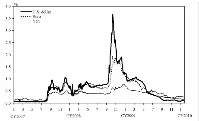
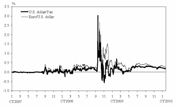
standing swap lines with the US Federal Reserve expanded to the Bank of England (BOE) and the BOJ. During this period, liquidity in the US dollar money markets outside the US quickly evaporated because of the sudden increase in the concerns over counterparty risk. LIBOR–OIS spreads increased substantially (Figure 1), and the financial strains were transmitted to the FX swap markets, as shown by the unusual increase in the spread of the FX-swap-implied dollar rate and LIBOR (3-month data) in Figure 2. Under such a situation, BOE, ECB, SNB and BOJ commenced the operations supplying US dollar funds at fixed rates within their appropriate collateral in October 2008. As Figure 3 shows, the amount of outstanding operations supplying US dollar funds increased sharply through the end of 2008.5 Thanks to the substantial provision of dollars in the markets outside the US, tightness in money markets and FX swap markets eased in 2009, as shown in Figure 1 and Figure 2. Faced with these improvements in the financial markets, the rates applied to the operations supplying US dollar funds rose above the market rates, and the amount of outstanding operations supplying US dollar funds declined through the first half of 2009 as Figure 3
3 Goldberg, Kennedy and Miu (2010) provide an excellent overview of the evolution of reciprocal currency
arrangements or dollar swap facilities that the Federal Reserve established with foreign central banks from 2007 to 2010.
4 Regarding empirical studies on the effectiveness of the TAF to reduce the strain in the short-term dollar
markets, see, for example, McAndrews et al. (2008), Taylor and Williams (2009), and Wu (2008). They reach different conclusions depending on the econometric identification assumptions.
5 Baba and Packer (2009) use data of foreign exchange swap pairs between the US dollar, euro, Swiss franc,
shows. On January 27, 2010, the Federal Open Market Committee announced that the temporary liquidity swap arrangements between the Federal Reserve and other central banks would expire on February 1. BOE, BOJ, ECB, and SNB announced the end of their US dollar-fund supplying operations the following day.
Given those developments, we show how the two temporary policy measures, the standing swap lines with the foreign central bank to supply foreign currency in the domestic market, and the acceptance of cross-border collateral arrangements, helped alleviate the liquidity shortages in the foreign currencies and improve the efficiency of the equilibrium in a two-country version model of Chapman and Martin (2007), which extends Freeman (1999).
Freeman (1999) examines the implication of aggregate default risk for the general equilibrium welfare effects of open market operations and discount windows. His model shows that open market operations not only reduce the risk to which the purchaser of the debt is exposed, but also spread aggregate risk more broadly and efficiently if all agents are risk averse, even if the central bank incurs losses related to default.
Chapman and Martin (2007) extend Freeman’s model by introducing moral hazard. Specifically, they point out that creditors’ incentives to monitor their loans would be reduced if the creditors knew that the central bank, which cannot monitor the quality of loans, would absorb losses under a “market-insensitive policy,” a policy whereby a central bank purchases the loans at a preannounced uniform discount rate, which Freeman (1999) recommends. Chapman and Martin (2007) show that a “market-sensitive policy,” a policy where a central bank randomly chooses a restricted number of creditors to compete for central bank funds, cures the shortcomings of the market-insensitive policy. By restricting the number of agents, the central bank limits the moral hazard problem because the creditors know that the creditors
are more likely to accept funds from other creditors who can check the quality of loans. By letting the creditors compete for central bank funds, the central bank exploits market information to infer the state of the economy because creditors bid up the price at which they borrow until the expected value of the loan is equal to the expected value of the collateral.
We extend the model of Chapman and Martin (2007) by adding the following five aspects: (1) some creditors want to consume goods produced by foreign debtors, (2) these creditors need foreign currency to purchase foreign debtors’ goods because foreign debtors only accept foreign currency, (3) to obtain foreign currency, these creditors first get second-hand debt denominated in foreign currency in exchange for their own currency-denominated loans in an active offshore international market (hereafter we call that offshore market the Eurodollar market, essentially a market for collateral swaps), (4) these creditors obtain foreign currency by presenting the second-hand debt to the issuer of the debt in the foreign credit market or by open market purchase by the foreign central bank, and (5) these creditors purchase foreign debtors’ goods using foreign currency (i.e. they undertake cross-border activity). These extensions allow us to examine two issues.
First, we examine the effects of domestic open market operations, which include lending to foreigners against domestic collateral. The optimal policy in normal times is the market-sensitive policy that Chapman and Martin (2007) propose. However, in our case, the market-sensitive policy in one country has positive spillover effects to risk averse creditors in the other country by mitigating the risk of liquidity shortages and default.
Second, we examine the effects of two temporary policy measures: standing swap lines with the foreign central bank to supply foreign currency in the domestic market, and the acceptance of cross-border collateral arrangements. Consider a sudden increase in the perceptions of counterparty risk in the Eurodollar market, which leads to a shutdown of all transactions, as we experienced in the Eurodollar market in early October 2008. Our model
shows central banks in two economies should take counterparty risks in the collateral swap market in one of the two temporary policy measures to improve the efficiency of market equilibrium. Specifically, the central banks should use the market-insensitive policy to substitute the transactions in the Eurodollar market when the creditors are reluctant to transact in this market. The market-insensitive policy could be either lending foreign currency to domestic agents against domestic collateral or lending domestic currency to foreign agents against foreign collateral. The central banks should supplement their market-insensitive policy in the Eurodollar market by their market-sensitive policy in their domestic credit markets. When the creditors resume transactions in the Eurodollar market, the central banks can exit from the market-insensitive policy in the Eurodollar market automatically. The automatic exits become possible because under the market-insensitive policy, the central banks set their discount rates slightly below the discount rates that would prevail under no monitoring effort by the creditors. These discount rates are inexpensive for the creditors in a situation in which a sudden increase in the perceptions of counterparty risk in the Eurodollar market leads to a shutdown of all transactions, but expensive for the creditors under normal market conditions.
The two temporary policy measures improve the welfare of both economies in a situation in which a sudden increase in the perceptions of counterparty risk in the Eurodollar market leads to a shutdown of all transactions, and thus these two temporary policy measures are incentive compatible to both central banks. The two temporary policy measures, however, cannot achieve the same level of efficiency as achieved by the foreign currency market transactions under normal conditions because central banks cannot use market-sensitive policy.
To the best of our knowledge, we are the first to show how the two temporary policy measures help alleviate liquidity crises in the foreign currencies in a theoretical model based
on Freeman (1999) and Chapman and Martin (2007).6
The rest of the paper is organized as follows. Section 2 explains the environment and trading patterns. Section 3 analyzes equilibrium with liquidity constraints. Section 4 considers the role of the market-sensitive policy and market-insensitive policy to mitigate the liquidity constraints in normal market conditions. Section 5 considers the role of the standing swap lines with the foreign central bank to supply foreign currency in the domestic market when the Eurodollar market is shut down. Section 6 studies the effects of cross-border collateral arrangements when the Eurodollar market is shut down. Section 7 discusses practical issues related to the two temporary policy measures, and Section 8 concludes.
2. Environment and trading patterns
2.1 The environment
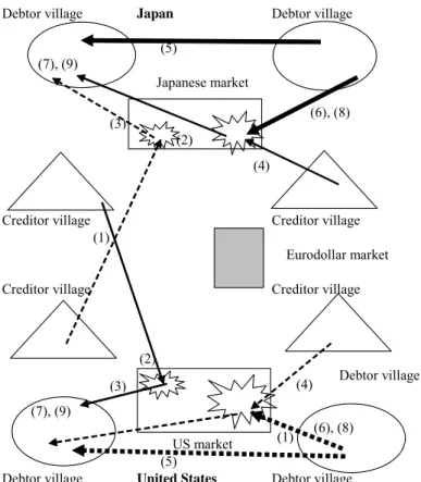
This section explains our model, which extends Chapman and Martin (2007) to a two-country model. There are two types of agents, called creditors and debtors, in the domestic country (hereafter Japan) and the foreign country (hereafter US). In both countries, creditors and debtors are scattered and live in small villages. Their populations are normalized to one, and their lifetime is divided into two periods. Japanese and US creditors and debtors are endowed with nonstorable goods specific to their villages in their first period of life, in the
6 There are many other ways to analyze the effects of liquidity crises on consumption in a multicountry model.
For example, Castiglionesi, Feriozzi and Lorenzoni (2009) use a multiregion version of the model of Diamond and Dybvig (1983) and show that financial integration reduces aggregate uncertainty and increases welfare, but induces banks to reduce their liquidity holdings, and that this increases the severity of extreme events. Regarding the cross-border use of collateral in payment systems, Manning and Willison (2006) examine the extent to which the liquidity risk arising from such a mismatch may be mitigated by allowing cross-border use of collateral in a two-country, two-bank model in which risk-neutral banks minimize expected costs with respect to their collateral choice in each country.
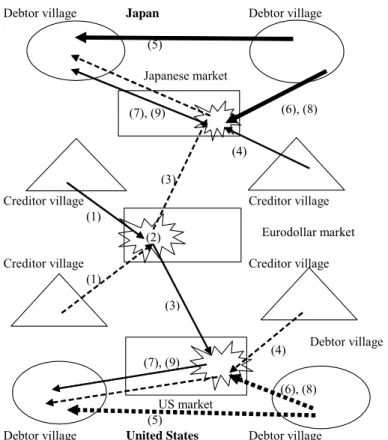
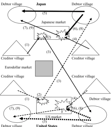
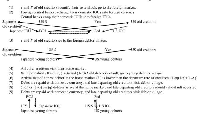
amounts of y,x,Y , and X respectively. Lowercase letters represent Japanese variables and uppercase letters represent US variables. The sequence of travel and trading patterns of debtors and creditors in each country during their lifetimes are summarized in Figure 4 and Figure 5, and we will explain them in turn below.
2.2 Trips by Japanese debtors and creditors
Japanese debtors consume their own endowment and Japanese creditor goods in the first period. At the beginning of the period, Japanese young debtors travel to the Japanese creditor village with which they are paired, where they may consume creditor village goods in exchange for the IOU to pay in yen in the second period at the Japanese market, where all IOUs denominated in yen are repaid. They return to their village of origin later in the period.
At the beginning of the second period, with probability θ, default occurs.
Specifically, (1−et)η debtors do not travel to the Japanese market, but scatter to Japanese
debtor villages where they are free to consume, and only 1–(1−et)η debtors travel to the Japanese market to pay their debt to the creditors, where et is the monitoring effort exerted by the Japanese creditors, which will be explained in the next paragraph. The default shock is independently and equally distributed over time and its realization is not known in advance.
η
) 1
( −et is the same for all debtors as long as creditors choose the same monitoring effort level et . With probability 1–θ, all debtors travel to the Japanese market to pay their debt to creditors. The function vc(ctd)+vd(dtd)+θ(1−et)η⋅vd(dtd+1) shows the expected utility of
Japanese debtors, where d
t
c , d
t
d and d
t
d+1 show the consumption of debtor and creditor
village goods when young, and of debtor village goods when old. The superscripts c and d
continuously differentiable strictly increasing concave functions. vc and vd have infinite
marginal utilities when their arguments are zero.
Japanese creditors consume c
t
c units of their own endowment when young, and when old, consume either c
t
d+1 units of Japanese debtor goods with probability (1–τ) or c t
D+1 units
of US debtor goods with probability τ. The utility of Japanese creditors is
), ( ) ( ) 1 ( ) ( 1 c1 t D c t d c t c c u d u D
u + −τ ⋅ + +τ⋅ + where the subscripts on the utility function denote
the types of goods consumed. The continuous and continuously differentiable utility functions uc and ud are strictly increasing and concave in each argument. Japanese creditors
invest effort et in monitoring the loan they extended to the debtor. Effort linearly decreases
the probability of default, and thus (1−et)η is the default probability they face if they invest
t
e . All creditors can verify the monitoring effort of the other creditors, but central banks
cannot. Japanese creditors get disutility from their effort of monitoring ϕ(et), where ϕ is an increasing concave function and ϕ(0)=0.
Japanese creditors know the types of goods to consume when old at the beginning of their second time period. (1–τ) creditors travel to the Japanese market. τ creditors first meet with T old US creditors, whose travel before their arrival to the Eurodollar market will be explained in the next paragraph, in the Eurodollar market, exchange the IOUs they have, and then travel to the US market. These US creditors travel from the Eurodollar market to the Japanese market holding Japanese IOUs.
Arrival at the Japanese market takes place in two stages. In the first stage, (1–τ) old Japanese creditors and T old US creditors, and λ old Japanese debtors arrive, where 0≤λ≤1 and 1–λ ≥ (1−et)η. At the end of the first stage, (1–α)(1–τ) old Japanese creditors and
the second stage. In the second stage, the remaining 1–λ–(1−et)η old debtors arrive if a
default shock occurs, and 1–λ old debtors arrive otherwise. The remaining creditors know whether a default occurs or not at this time.
All creditors face the same probability of leaving the Japanese market early ((1–α) for Japanese creditors and (1–A) for US creditors), and all debtors face the same probability of arriving early, late or not at all. Each learns his/her arrival or departure time as soon as he/she turns old. After the visit to the Japanese market, (1–τ) Japanese creditors, T US creditors and old debtors who have not gone to the Japanese market (and thus defaulted) randomly scatter to a selected Japanese debtor island. They arrive at the debtor island after the trips made by the creditors are completed.
2.3 Trips by US debtors and creditors
US debtors consume their own endowment and US creditor goods in the first period. At the beginning of the period, US young debtors travel to the creditor village with which they are paired, where they may consume creditor village goods in exchange for the IOU to pay in dollar the second period at the US market, where all IOUs denominated in dollar are repaid. They return to their debtor villages later in the period. With probability Θ, (1−Et)Η debtors do not travel to the US market, but scatter to US debtor villages where they are free to consume. Et is the monitoring effort exerted by the US creditors, which will be explained in
detail in the next paragraph. With probability 1–Θ, all debtors travel to the US market. The default shock is independently and equally distributed over time and its realization is not
known in advance. The function VC(CtD)+VD(DtD)+Θ(1−Et)Η⋅VD(DtD+1) shows the expected utility of US debtors.7
US creditors consume C
t
C units of their own endowment when young and either
C t
D+1 units of US debtor goods with probability (1–T) or C t
d+1 units of Japanese debtor goods
when old with probability T. The utility of US creditors is
) ( ) ( ) 1 ( ) ( 1 C1 t d C t D C t C C T U D T U d
U + − ⋅ + + ⋅ + .8 US creditors invest effort Et in monitoring the
loan they extended to the debtor. Effort linearly decreases the probability of default, and thus (1−Et)Η is the default probability they face if they invest Et . All creditors can verify the effort of monitoring, but central banks cannot. US creditors get disutility from their monitoring effort Φ(Et), where Φ is an increasing concave function and Φ(0)=0.
US creditors know the types of goods to consume when old at the beginning of their second time period. (1–T) creditors travel to the US market. T creditors first meet with τ old Japanese creditors in the Eurodollar market, exchange the IOUs they have, and then travel to the Japanese market.
After the visit to the US market, (1–T) old US creditors, along with τ old Japanese creditors and defaulted old US debtors randomly select US debtor islands.
Arrival at the US market takes place in two stages. In the first stage, (1–T) old US creditors, τ old Japanese creditors and Λ old US debtors arrive, where 0≤Λ≤1 and 1–Λ ≥
Η
− )
1
( Et . At the end of the first stage, (1–α)τold Japanese creditors and (1–A)(1–T) old US
creditors leave for their final destination, while the rest remain until the end of the second
7 D t
C , DtD and DtD+1 represent their consumption of debtor and creditor village goods when young and of
debtor village goods when old. The functions VC and VD are continuous and continuously differentiable strictly
increasing concave. VC and VDhave infinite marginal utilities when their arguments are zero.
8 The continuous and continuously differentiable utility functions U
C and UD are strictly increasing and concave
stage. In the second stage, the remaining 1–Λ–(1−Et)Η old debtors arrive if a default shock
occurs, and 1–Λ old debtors arrive otherwise. The remaining creditors know whether a
default occurs or not at this time.
All creditors face the same probability of leaving early in the US market ((1–α) for Japanese creditors and (1–A) for US creditors), and all debtors face the same probability of arriving early, late or not at all. Each learns his/her arrival or departure time as soon as he/she turns old.
2.4 Trading patterns
There exist central banks in the Japanese market and US market that issue currency with initial stocks of m yen and M dollars to each initial old creditor, whose mass is one and who lives only in the first period.
All agents can issue unfalsifiable IOUs that identify the issuer. Regal authorities exist in the Japanese market and US market and enforce the agreements between the parties currently in the villages. Regal authorities do not exist to enforce agreements in the Eurodollar market and at the agents’ final destination.
To consume when old, creditors must bring something of value to the debtor island. Currency will be accepted by young debtors if it helps them to pay their debts and thereby to acquire the goods they desire. If it is accepted in equilibrium, creditors will require that debts be repaid with currency.
The young debtors wish to consume goods from creditors’ villages but do not have national currency at hand. The young debtors offer creditors a promise to pay a sum of money in the next period in the domestic market. Because of the extent of legal authority, we assume that debtors can only promise to pay in national currency. The young debtor will
acquire this money by selling some of his/her endowment to an old creditor who brings domestic currency to the village later in the period.
Given this sequence of trade, the old creditors who want to consume foreign goods in the second period need foreign currency. To obtain foreign currency, the old creditors must exchange their national IOUs for foreign IOUs in the Eurodollar market. While the exchange of IOUs in this model is for the sake of consumption by the old creditors in foreign economies, the exchange could be interpreted as foreign currency funding in the offshore money market by multinational banks. Money is essential to make final payment to retire debt, and without repayment in the national currency, creditors will not accept debt.
Debts are cleared at the national market but not always bilaterally. Because the arrival rate of the old debtors is lower than the departure rate of old creditors, the early-departing old creditors sell their yet-unredeemed debt to the late-departing old creditors. The amount of debt redeemed in this second-hand debt market is limited by the currency that the early-arriving old debtors bring to the market, and thus the second-hand debt may be traded at a discount value.
In summary, creditors need to think about eight trading patterns, depending on whether they consume foreign goods or not, whether they depart the market early or late, and whether default occurs or not. Debtors need to consider two trading patterns, depending on whether default occurs. Note that whether a debtor arrives in the market early or late when old does not affect his/her consumption. Only whether he/she defaults or not affects his/her additional consumption when old. The probability of default of debtors in Japan and US is independent, and we have four states: state 00, with probability (1–θ)(1–Θ) of no default in both economies; state 10, with probability θ (1–Θ) that only Japanese debtors default; state 01, with probability ((1–θ)Θ) that only US debtors default; state 11, with probability (θΘ) that both Japanese and US debtors default. Those events are identified only after the arrival
of all debtors in each market. The situation of default in one economy will be known to the other economy immediately. When we need to distinguish the level of choice variables in these four states, we will use the expressions x[00], x[01], x[10], x[11] to represent the value of variable x in states 00, 01, 10, and 11.
3. Equilibrium
This section first examines the optimization problem by debtors and creditors and then moves on to present the market equilibrium conditions and finally defines a symmetric laissez-fare equilibrium with liquidity constraints.
3.1 The Japanese debtor’s problem
Let pt be the yen price of Japanese debtor goods in Japanese debtor villages at time t.
Because only debtor goods are sold in exchange for money in the current period, the yen price of Japanese debtor goods is a measure of the price level. Let mt be the acquisition of
yen from old creditors in exchange for debtor goods, let πt be the price of creditor island
goods at t of a promise to pay one yen on the Japanese market at t+1, and let ht be nominal
value at t of the Japanese debtor’s indebtedness. The Japanese debtor faces the following budget constraints: t d t t tx pd m p = + , (1) t t h m = , (2) t t d t h c = π , (3) t d t t d t t e p e m p+1[10] +1[10]= +1[11] +1[11]= . (4)
Note that equations (1) through (3) take into account the fact that all yen will be acquired by the young debtor in states 00, 10, 01 and 11 and thus his/her consumption
decision at time t does not depend on the states of default However, his/her consumption at time t+1 takes place only when default occurs in Japan (state 10, and 11) as can be seen in equation (4). Inserting those constraints into the utility function, the Japanese debtor maximizes: ) ] 11 [ ( ) -(1 ) ] 10 [ ( ) -)(1 -(1 ) ( ) ( 1 1 + + ⋅ Θ + ⋅ Θ + − + t t d t t t d t t t d t t c p m v e p m v e p m x v m v π θ η θ η , (5) by the choice of mt.
The resulting first-order condition will be:
0 ] 11 [ ' ) 1 ( ] 10 [ ' ) -(1 ) 1 ( ' ' 1 1 = ⋅ Θ − + ⋅ Θ − + − + + t d t t d t t d t c p v e p v e p v v π θ η θ η , (6)
where primes indicate first derivatives.
3.2 The US debtor’s problem
The US debtor’s problem is a mirror image of the Japanese debtor’s problem. Let Pt be the
dollar price of US debtor goods in the US debtor village at time t. Let Mt be the acquisition
of dollars from old creditors in exchange for debtor goods, let Πt be the price in creditor
island goods at t of a promise to pay one dollar in the US market at t+1, and let Ht be the
nominal value at t of the US debtor’s indebtedness. The US debtor faces the following
budget constraints: t D t t tX PD M P = + , (7) t t H M = , (8) t t D t H C = Π , (9) t D t t D t t E P E M P+1[01] +1[01]= +1[11] +1[11]= . (10)
) ] 11 [ ( ) 1 ( ) ] 01 [ ( ) 1 ( ) 1 ( ) ( ) ( 1 1 + + ⋅ Η − Θ + ⋅ Η − Θ − + − + Π t t D t t t D t t t D t t C P M V E P M V E P M X V M V θ θ , (11) by the choice of Mt.
The resulting first-order condition will be:
0 ] 11 [ ' ) 1 ( ] 01 [ ' ) 1 ( ) 1 ( ' ' 1 1 = ⋅ Η − Θ + ⋅ Η − Θ − + − Π + + t D t t D t t D t C P V E P V E P V V θ θ . (12)
3.3 The Japanese creditor’s problem
Let lt be the nominal value of a creditor’s loans to debtors at time t. Let qtc+1 (yen) and qtC+1
(yen) be the par value of nominal debt purchased by Japanese and US late-leaving creditors at time t+1. Let ρt+1≤1 represent the nominal price at which one yen of that debt is exchanged in the first stage of visits in the Japanese market at t+1. If default occurs, (1–λ–(1–et)η)/(1–λ)is the proportion of the remaining debt that will be repaid. Finally, let st
be the foreign exchange rate of yen per dollar that prevails in the Eurodollar market.
Similarly, let Lt be the nominal value of a creditor’s loans to debtors at time t. Let
C t
Q+1 (dollars) and c t
Q+1 (dollars) be the par value of nominal debt purchased by US and
Japanese late-leaving creditors at time t+1. Let Rt+1≤1 represent the nominal price at which one dollar of that debt is exchanged in the first stage of visits in the US market at t+1. If default occurs, (1–Λ–(1–Et)H)/(1–Λ) is the proportion of the remaining debt that will be
repaid. Those notations should be defined here because some of the Japanese creditors participate in the US second-hand debt market.
Japanese creditors consume c
t
c units of their own endowment when young. When
old, they consume either c t
d+1 units of Japanese debtor goods with probability (1–τ) or c t
D+1
units of US debtor goods with probability τ. The budget constraint of a Japanese creditor born at t when young is:
t t c t l c y= + π . (13)
Depending on whether he/she departs the market early or late, whether he/she consumes foreign goods or not, and whether the event of default occurs or not, a Japanese creditor has the following four budget constraints when old.
First, if he/she departs early and consumes Japanese goods (with probability of (1–α)(1–τ)) then: 11 , 01 , 10 , 00 ], [ ] [ ) 1 ( 1 1 1 − + = + + = + lt lt pt j dtc j j t λ λ ρ . (14)
Second, if he/she departs early and consumes US goods (with probability of (1–α)τ) then: 11 , 01 , 10 , 00 ], [ ] [ ) 1 ( 1 1 1 1 1 −Λ + +Λ + = + + = + l s l s P j D j j R c t t t t t t t . (15)
Equation (15) incorporates the fact that they exchange their yen-denominated loans into dollar-denominated loans at the beginning of time t+1 at the exchange rate st+1.
Third, if he/she departs late and consumes Japanese goods (with probability of
α(1–τ)) then, without default and with default, respectively, we have: 01 , 00 ], [ ] [ ) 1 ( − 1 1 = 1 1 = + + q+ p+ j d + j j l c t t c t t t ρ , if no default in Japan, (16) 11 , 10 ], [ ] [ 1 ) 1 ( 1 ) ) 1 ( 1 ( 1 − − 1 1= 1 1 = − − − + − − et lt qtc+ λ et ρt+qtc+ pt+ j dtc+ j j η λ η ,
if default occurs in Japan.
(17)
Finally, if he/she departs late and consumes US goods (with probability of ατ) then, without default and with default, respectively, we have:
10 , 00 ], [ ] [ ) 1 ( 1 1 1 1+ − + 1 = + + = + R Q+ P j D j j s l c t t c t t
t t , if no default in the US, (18)
11 , 01 ], [ ] [ 1 ) 1 ( 1 ) ) 1 ( 1 ( 1 1 − 1 1= 1 1 = Λ − Η − − Λ − + Η − − Et ltst+ Qtc+ Et Rt+Qtc+ Pt+ j Dtc+ j j ,
if default occurs in the US.
Using the budget constraints at times t and t+1 yields the following optimization problem for the young Japanese creditors with respect to lt, qtc+1, Qtc+1 and et at time t:
) ( ) ] [ ) 1 / ) 1 ( 1 ( ) ) 1 ( 1 ( ( Prob[j] ) ] [ ) 1 ( ( Prob[j] ) ] [ ) 1 / ) 1 ( 1 ( ) ) 1 ( 1 ( ( Prob[j] ) ] [ ) 1 ( ( Prob[j] ) 1 ( ) ] [ ) 1 ( ( Prob[j] ) 1 ( ) ] [ ) 1 ( ( Prob[j] ) 1 )( 1 ( ) ( 1 1 1 1 1 11 , 01 1 1 1 1 10 , 00 1 1 1 1 11 , 10 1 1 1 01 , 00 1 1 1 1 11 , 01 , 10 , 00 1 1 11 , 01 , 10 , 00 , , , 1 1 t t c t t c t t t t t D j t c t t t t D j t c t t c t t t t d j t c t t t d j t t t t t t D j t t t t d j t t c e Q q l e j P Q R Q E s l E u j P Q R s l u j p q q e l e u j p q l u j P s l s l R u j p l l u l y u Max t c t c t t ϕ τα ρ λ η λ η ρ α τ α τ λ λ ρ α τ π − − Λ − Η − − Λ − + Η − − ∑ + − + ∑ ⋅ + − − − − − + − − ∑ + − + ∑ ⋅ − + Λ + Λ − ∑ ⋅ − + + − ∑ ⋅ − − + − + + + + + = + + + + = + + + + = + + + = + + + + = + + = + + . (20)
Therefore, the first-order condition of this problem for lt is:
0 ] [ ) ) 1 ( 1 ( ) ] [ 1 ) 1 ( 1 ( ) ) 1 ( 1 ( ( ' Prob[j] ] [ ) ] [ ) 1 ( ( ' Prob[j] ] [ ) 1 ( 1 ) ] [ ) 1 / ) 1 ( 1 ( ) ) 1 ( 1 ( ( ' Prob[j] ] [ 1 ) ] [ ) 1 ( ( ' Prob[j] ) 1 ( ] [ ) 1 ( ) ] [ ) 1 ( ( ' Prob[j] ) 1 ( ] [ ) 1 ( ) ] [ ) 1 ( ( ' Prob[j] ) 1 )( 1 ( ) ( ' ) ( 1 1 1 1 1 1 1 11 , 01 1 1 1 1 1 1 10 , 00 1 1 1 1 1 11 , 10 1 1 1 1 01 , 00 1 1 1 1 1 1 1 1 11 , 01 , 10 , 00 1 1 1 1 11 , 01 , 10 , 00 = Η − − − Λ − Η − − Λ − + Η − − ∑ + + − ∑ ⋅ + − − − − − − − + − − ∑ + + − ∑ ⋅ − + Λ + Λ − Λ + Λ − ∑ ⋅ − + + − + − ∑ ⋅ − − + − − + + + + + + + = + + + + + + = + + + + + = + + + + = + + + + + + + + = + + + + = j P s E j P Q R Q E s l E u j P s j P Q R s l u j p e j p q q e l e u j p j p q l u j P s s R j P s l s l R u j p j p l l u l y u t t t t c t t c t t t t t D j t t t c t t t t D j t t t c t t c t t t t d j t t c t t t d j t t t t t t t t t t D j t t t t t t d j t t c t τα η ρ λ η λ η ρ α τ α τ λ λ ρ λ λ ρ α τ π π . (21)
The first-order condition for c t q+1 is: ) ] [ 1 ) 1 ( 1 )( ] [ 1 ) 1 ( 1 ) ) 1 ( 1 ( ( ' Prob[j] ] [ ) 1 ( ) ] [ ) 1 ( ( ' Prob[j] 0 1 1 1 1 1 1 11 , 10 1 1 1 1 1 01 , 00 j p e j p q q e l e u j p j p q l u t t t t c t t c t t t t d j t t t c t t t d j + + + + + + = + + + + + = − − − − − − − − − − + − − ∑ + − − + ∑ = ρ λ η λ ρ λ η λ η ρ ρ . (22)
The first-order condition for c t
] [ ) 1 ) 1 ( 1 ( ) ] [ 1 ) 1 ( 1 ) ) 1 ( 1 ( ( ' Prob[j] ] [ ) 1 ( ) ] [ ) 1 ( ( ' Prob[j] 0 1 1 1 1 1 1 1 11 , 01 1 1 1 1 1 1 10 , 00 j P R E j P Q R Q E s l E u j P R j P Q R s l u t t t t c t t c t t t t t D j t t t c t t t t D j + + + + + + + = + + + + + + = − Λ − Η − − Λ − − Λ − Η − − Λ − + Η − − ∑ + − − + ∑ = . (23)
The first-order condition for et is:
) ( ) ] [ 1 ( ) ] [ 1 ) 1 ( 1 ) ) 1 ( 1 ( ( Prob[j] ) 1 ( 1 1 1 1 1 1 11 , 10 t t c t t t c t t c t t t t d j p j e q l j p q q e l e u η λ ϕ ρ λ η λ η α τ − − ⋅ + − = ′ − − − + − − ′ ∑ ⋅ − + + + + + + = . (24)
3.4 The US creditor’s problem
US creditors consume C
t
C units of their own endowment when young. When old, they
consume either C
t
D+1 units of US debtor goods with probability (1–T) or C t
d +1 units of Japanese debtor goods with probability T. The budget constraint of a US creditor born at t
when young is:
t t C t L C Y = + Π . (25)
Depending on whether he/she departs the market early or late, whether he/she consumes foreign goods or not, and whether default occurs or not, a US creditor has the following budget constraints when old.
First, if he/she departs early and consumes US goods (with probability of (1–A)(1–T)) then: 11 , 01 , 10 , 00 ], [ ] [ ) 1 ( 1 1 1 −Λ +Λ = + + = + L L P j D j j R C t t t t t . (26)
Second, if he/she departs early and consumes Japanese goods (with probability of (1–A)T) then: 11 , 01 , 10 , 00 ], [ ] [ ) 1 ( 1 1 1 1 1 − + = = + + + + + p j d j j s L s L c t t t t t t t λ λ ρ . (27)
Third, if he/she departs late and consumes US goods (with probability of A(1–T)) then, without default and with default, respectively, we have:
10 , 00 ], [ ] [ ) 1 ( − 1 1 = 1 1 = + R+ Q+ P+ j D+ j j L C t t C t t
t , if no default occurs in the US, (28)
11 , 01 ], [ ] [ 1 ) 1 ( 1 ) ) 1 ( 1 ( 1 − 1 1= 1 1 = Λ − Η − − Λ − + Η − − E L Q+ E R+Q+ P+ j DC+ j j t t C t t t C t t t ,
if default occurs in the US.
(29)
Finally, if he/she departs late and consumes Japanese goods (with probability of AT) then, without default and with default respectively, we have:
01 , 00 ], [ ] [ ) 1 ( 1 1 1 1 1 = = − + + + + + + j j d j p q s L C t t C t t t
t ρ , if no default occurs in Japan, (30)
11 , 10 ], [ ] [ 1 ) 1 ( 1 ) ) 1 ( 1 ( 1 1 1 1 1 1 = = − − − − − + − − + + + + + + j j d j p q e q s L e C t t C t t t C t t t tη λ λ η ρ ,
if default occurs in Japan.
(31)
Using the budget constraints at times t and t+1 yields the following optimization problem for the young US creditors with respect to Lt, QtC+1, qtC+1 and Et at time t:
) ( ) ] [ 1 ) 1 ( 1 ) ) 1 ( 1 ( ( Prob[j] ) ] [ ) 1 ( ( Prob[j] ) ] [ 1 ) 1 ( 1 ) ) 1 ( 1 ( ( Prob[j] ) ] [ ) 1 ( ( Prob[j] ) 1 ( ) ] [ ) 1 ( ( Prob[j] ) 1 ( ) ] [ ) 1 ( ( Prob[j] ) 1 )( 1 ( ) ( 1 1 1 1 1 11 , 10 1 1 1 1 01 , 00 1 1 1 1 11 , 01 1 1 1 10 , 00 1 1 1 11 , 01 , 10 , 00 1 1 11 , 01 , 10 , 00 , , , 1 1 t t C t t C t t t t t d j t C t t t t d j t C t t C t t t t D j t C t t t D j t t t t t d j t t t t D j t t C E q Q L E j p q q e s L e U j p q s L U TA j P Q R Q E L E U j P Q R L U A T s j p L L U A T j P L L R U A T L Y U Max t C t C t t Φ − − − − − − + − − ∑ + − + ∑ ⋅ + − Λ − Η − − Λ − + Η − − ∑ + − + ∑ ⋅ − + + − ∑ ⋅ − + Λ + Λ − ∑ ⋅ − − + Π − + + + + + = + + + + = + + + + = + + + = + + + = + + = + + ρ λ η λ η ρ λ λ ρ . (32)
0 ] [ ) ) 1 ( 1 ( ) ] [ 1 ) 1 ( 1 ) ) 1 ( 1 ( ( ' Prob[j] ] [ 1 ) ] [ ) 1 ( ( ' Prob[j] ] [ ) ) 1 ( 1 ( ) ] [ 1 ) 1 ( 1 ) ) 1 ( 1 ( ( ' Prob[j] ] [ 1 ) ] [ ) 1 ( ( ' Prob[j] ) 1 ( ] [ ) 1 ( ) ] [ ) 1 ( ( ' Prob[j] ) 1 ( ] [ ) 1 ( ) ] [ ) 1 ( ( ' Prob[j] ) 1 )( 1 ( ) ( ' 1 1 1 1 1 1 1 11 , 10 1 1 1 1 1 1 01 , 00 1 1 1 1 1 11 , 01 1 1 1 1 10 , 00 1 1 1 1 1 1 11 , 01 , 10 , 00 1 1 1 1 11 , 01 , 10 , 00 = − − − − − − − + − − ∑ + − + ∑ ⋅ + Η − − − Λ − Η − − Λ − + Η − − ∑ + − + ∑ ⋅ − + − + − ∑ ⋅ − + Λ + Λ − Λ + Λ − ∑ ⋅ − − + Π − Π − + + + + + + + = + + + + + + = + + + + + = + + + + = + + + + + + = + + + + = t t t t C t t C t t t t t d j t t t C t t t t d j t t t C t t C t t t t D j t t C t t t D j t t t t t t t t d j t t t t t t D j t t C t s j p e j p q q e s L e U s j p j p q s L U TA j P E j P Q R Q E L E U j P j P Q R L U A T s j p s j p L L U A T j P R j P L L R U A T L Y U η ρ λ η λ η ρ λ ρ λ λ ρ . (33)
The first-order condition for C t Q+1is: ] [ 1 ) 1 ( 1 ) ] [ 1 ) 1 ( 1 ) ) 1 ( 1 ( ( ' Prob[j] ] [ ) 1 ( ) ] [ ) 1 ( ( ' Prob[j] 0 1 1 1 1 1 1 11 , 01 1 1 1 1 1 10 , 00 j P R E j P Q R Q E L E U j P R j P Q R L U t t t t C t t C t t t t D j t t t C t t t D j + + + + + + = + + + + + = − Λ − Η − − Λ − − Λ − Η − − Λ − + Η − − ∑ + − − + ∑ = . (34)
The first-order condition for C t q+1 is: ] [ 1 ) 1 ( 1 ) ] [ 1 ) 1 ( 1 ) ) 1 ( 1 ( ( ' Prob[j] ] [ ) 1 ( ) ] [ ) 1 ( ( ' Prob[j] 0 1 1 1 1 1 1 1 11 , 10 1 1 1 1 1 1 01 , 00 j p e j p q q e s L e U j p j p q s L U t t t t C t t C t t t t t d j t t t C t t t t d j + + + + + + + = + + + + + + = − − − − − − − − − − + − − ∑ + − − + ∑ = ρ λ η λ ρ λ η λ η ρ ρ . (35)
The first-order condition for Et is:
) ( ] [ 1 ) ] [ 1 ) 1 ( 1 ) ) 1 ( 1 ( ( Prob[j] ) 1 ( 1 1 1 1 1 1 11 , 01 t t C t t t C t t C t t t t D j P j E Q L j P Q R Q E L E U A T −Λ − Η + −Λ =Φ ′ Η − − Λ − + Η − − ′ ∑ ⋅ − + + + + + + = . (36)
3.5 Market clearing conditions
The conditions for the clearing of the market of goods denominated in yen and dollars in debtor villages are:
) ( d t t x d p m= − , (37) ) ( D t t X D P M = − . (38)
Note that young debtors at time t are not affected by whether old debtors have
defaulted, which implies the existence of an equilibrium in which a debtor’s demands for real balances do not depend on the realization of the default shock. Moreover, the same number of nominal yen and dollars arrive in each village (either brought by old creditors or old debtors) whether or not a default has occurred. Hence, equations (37) and (38) imply that the price levels are the same whether a default shock has occurred or not.
The clearing of the market for loans in yen and dollars requires: t t l h = , (39) t t L H = . (40)
These equations determine the price levels pt and Pt, the period t goods’ price of debt
payable in period t+1, πt and Πt.
In the Eurodollar market, T US creditors andτ Japanese creditors exchange their loans. We assume that the exchange will occur on a pro rata basis, because creditors supply their loans inelastically. The nominal exchange rate will be determined to equate the nominal value of the transactions:
T L s
lt⋅ t+1⋅τ = t⋅ . (41)
Per capita holding of foreign loans in domestic currency becomes TLt τ dollars for Japanese creditors and τlt T yen for US creditors.
Equation (42) below shows that in the Japanese resale market for loans, the sum of the debt purchased by the α(1–τ) Japanese late-leaving creditors, c
t
creditors, C t
q , must equal the unredeemed debt, which is the sum of the proportions (1–λ) of debt owned by the (1–α)(1–τ) Japanese early-leaving creditors, (1–λ)(1–α)(1–τ)lt, and the
proportion (1–λ) of debt owned by the (1–A)T US early-leaving creditors,
(1–λ)(1–A)T(τ T )lt = (1–λ)(1–A)τlt:
[
]
t C t c t ATq A l q (1 )(1 ) (1 ) (1 ) ) 1 ( τ 1 1 α τ τ λ α − + + + = − − + − − . (42)The other constraint in the Japanese resale market for loans is that the amount of yen
available to repurchase the debt, c
t c t+1q+1 ρ and C t C t+1q+1
ρ , is limited by the amount of yen
delivered by the early-arriving debtors, λlt as follows:
C t C t c t c t t q q l ≥ρ+1 +1+ρ+1 +1 λ . (43)
In the US resale market for loans, the sum of the debt purchased by the US A(1–T) late-leaving creditors, C
t
Q , and ατ Japanese late-leaving creditors, c
t
Q , must equal the
unredeemed debt, which is the sum of the proportion (1–Λ) of debt owned by the (1–A)(1–T) US early-leaving creditors, (1–Λ)(1–A)(1–T)Lt, and the proportion (1–Λ) of debt owned by
the (1–α)τJapanese early-leaving creditors, (1–Λ)(1–α)τ (TLt/τ) = (1–Λ)(1–α) TLt, as shown
in equation (44) below:
[
]
t C t c t A T Q A T T L Q+1+ (1− ) +1 = (1− )(1− )+(1−α) (1−Λ) ατ . (44)The other constraint in the US resale market for loans is that the amount of dollars
available to repurchase the debt, C
t C t Q R+1 +1 and c t c t Q
R+1 +1, is limited by the amount of dollars delivered by the early-arriving debtors, ΛLt as follows:
c t c t C t C t t R Q R Q L ≥ +1 +1+ +1 +1 Λ . (45)
3.6 Symmetric laissez-fare equilibrium with liquidity constraints
Consider a symmetric laissez-fare equilibrium where both Japanese and US liquidity constraints (equations (43) and (45)) are binding and all the same types of Japanese and US creditors choose the same actions, and central banks do not intervene in the markets. Note that equations (37) and (38) imply that the price levels are the same whether or not a default shock has occurred. Taking these properties into consideration, let pt+1[j] = pt+1 = p, ρt+1 = ρ,
ps = 1/πp, ls = l/p, hs = h/p, ms = m/p, mπ = (m/p)(πp) = ms/ps, qsc = qc/ps, qsC = qC/ps and et =
es for Japan, and let Pt+1[j] = Pt+1 = P, Rt+1 = R, Ps = 1/ΠP, Ls = L/P, Hs = H/P, Ms = M/P, MΠ
= Ns/Ps, Qsc = Qc/Ps, QsC = QC/Ps and Et = Es for the US. For the sake of expressing the
discount rate (the nominal price at which one dollar of that debt is exchanged in the first stage of visits on the domestic market at t+1) in the demand schedule of creditors, we will use the notation ρc, ρC, Rc, and RC.
Using these notations and equilibrium conditions in the loan and money markets, equations (2) and (39), and ls = hs = ms, we can simplify the first-order conditions for
Japanese agents as follows. In particular, equations (6), (21), (22), (23), and (24) would be simplified as follows: 0 ) ( ' ) 1 ( ) ( ' ) ( ' 1 − − + − = s d s s d s s c s l v e l x v p l v p θ η , (46)
{
}
−Θ + − +Θ − − Η + − − Η −Λ − − − Η ⋅ + − − − − − − + − − + − + − ⋅ − + Λ + Λ − Λ + Λ − ⋅ − + + − + − ⋅ − − = − P ps E Q R E l E u P ps Q R l u e q e l e u q l u P ps R P ps l R u l l u p l y u p s c s c s s s D c s c s D s c s c s s s d c s c s d C s C D c s s c d s s c s ) ) 1 ( 1 ]( ) ) 1 /( ) 1 ( 1 ( ) ) 1 ( 1 [( ' ) ]( ) 1 ( [' ) 1 ( ) ) 1 ( 1 ]( ) ) 1 /( ) 1 ( 1 ( ) ) 1 ( 1 [( ' ) ) 1 ( ( ' ) 1 ( ) 1 ( ) }( ) 1 ( )]{ ( } ) 1 ( [{ ' ) 1 ( ] ) 1 ( ][ ) 1 ( [' ) 1 )( 1 ( ) ( ' ) 1 ( τα η ρ λ η η θ ρ θ α τ α τ λ λ ρ λ λ ρ α τ (47) ) 1 ) 1 ( 1 ]( ) 1 ) 1 ( 1 ( ) ) 1 ( 1 [( ' ) 1 ]( ) 1 ( [' ) 1 ( 0 c s c c s s s d c c s c s d e q e l e u q l u ρ λ η ρ λ η η θ ρ ρ θ − − − − − − − − + − − + − − + − = , (48)) 1 ) 1 ( 1 ]( ) 1 ) 1 ( 1 ( ) ) 1 ( 1 [( ' ) 1 ]( ) 1 ( [' ) 1 ( 0 c s c s c s s s D c c s c s D R E P ps Q R E l E u R P ps Q R l u − Λ − Η − − − Λ − Η − − + Η − − Θ + − − + Θ − = , (49) ) ( ) 1 ( ] ) ) 1 ( ) 1 ( 1 ( ) ) 1 ( 1 [( ' ) 1 ( cs s s c s c s s s d e l e q l q e u ϕ λ η ρ λ η λ η θ α τ = ′ − + − − − − − + − − ⋅ − . (50)
Equation (42), the equilibrium condition of the Japanese resale market for loans, becomes:
[
]
s C s c s ATq A l q (1 )(1 ) (1 ) (1 ) ) 1 ( τ α τ τ λ α − + = − − + − − . (51)The liquidity constraint in the Japanese resale market for loans becomes: C s C c s c s q q l ρ ρ λ ≥ + . (52)
Next, we can simplify the first-order conditions for US agents as follows. In particular, equations (12), (33), (34), (35), and (36) after using the equilibrium conditions in the loan and money markets, equations (8) and (40), and Ls = Hs = Ms, become:
0 ) ( ' ) 1 ( ) ( ' ) ( ' 1 − − +Θ − Η = s D s s D s s C s L V E L X V P L V P , (53) − − − − − − + − − + − + − ⋅ + − − − Η Λ − Η − − + Η − − Θ + − + Θ − ⋅ − + + − + − ⋅ − + Λ + Λ − Λ + Λ − ⋅ − − = − ps P e ps P q e L e U ps P ps P q L U TA E Q R E L E U Q R L U A T ps P ps P L U A T R L R U A T P L Y U P s C s C s s s d C s C s d s C S C s S s D C s C S D C S C d C S C D s s C s ) ) 1 ( 1 )( }] ) 1 ) 1 ( 1 ( ) ) 1 ( 1 [{( ' ] } ) 1 ( [{ ' ) 1 ( ) ) 1 ( 1 ])( ) 1 ) 1 ( 1 ( ) ) 1 ( 1 [( ' ] ) 1 ( [' ) 1 ( ) 1 ( } ) 1 ( ]{ } ) 1 ( [{ ' ) 1 ( } ) 1 ( ]{ } ) 1 ( [{ ' ) 1 )( 1 ( ) (' 1 η ρ λ η η θ ρ θ λ λ ρ λ λ ρ , (54) ) 1 ) 1 ( 1 ]( ) 1 ) 1 ( 1 ( ) ) 1 ( 1 [( ' ) 1 ]( ) 1 ( [' ) 1 ( 0 C s C S s S s D C C S C S D R E Q E L E U R Q R L U − Λ − Η − − Λ − Η − − + Η − − Θ + − − + Θ − = , (55) ) 1 ) 1 ( 1 )( ]( ) 1 ) 1 ( 1 ( ) ) 1 ( 1 [( ' ) 1 )( }( ) 1 ( [{ ' ) 1 ( 0 C s C S C s S s d C C S C S d e ps P q e L e U ps P q L U ρ λ η ρ λ η η θ ρ ρ θ − − − − − − − − + − − + − − + − = , (56) ) ( ) 1 ( ] ) 1 ) 1 ( 1 ( ) ) 1 ( 1 [( ' ) 1 ( S C S s C S C s S s D E Q L Q R E L E U A T =Φ′ Λ − + Η − Λ − Η − − Λ − + Η − − Θ ⋅ − . (57)
Equation (44), the equilibrium condition of the US resale market for loans becomes:
[
]
S C S c s A T Q A T T L Q + (1− ) = (1− )(1− )+(1−α) (1−Λ) ατ . (58)Equation (45), the liquidity constraint in the US resale market for loan becomes: c c C C S R Q R Q L ≥ + Λ . (59)
Finally, the equilibrium condition in the Eurodollar market, equation (41), becomes: τ ⋅ ⋅ = s s l T L P ps . (60)
We obtain the equilibrium in the following way. First, by inserting the left-hand side of equation (60) into equations (47), (49), (54), and (56), we can eliminate the terms of trade, (ps/P). Then we use 14 equations, i.e. (46) through (59), to solve for 14 unknowns, ps, ls, qsc,
Qsc, ρc, Rc, es, Ps, Ls, qsC, QsC, ρC, RC and Es. Second, using equilibrium conditions in the
money market ms =m/p=m/p and Ms =M/P=M /P, we solve for p and P given ms ,
Ms, m, and M . Finally, using equation (60), ls, Ls, p and P, we obtain s.
Note that competition in the resale market for loans implies three possibilities: ρc = ρC,
qsc >0 and qsC>0 or ρc>ρC; qsc >0 and qsC = 0, or ρc<ρC, qsc = 0; and qsC>0. Similar
conditions apply to the US resale market for loans. Furthermore, equations (48), (49), (54),
and (55) show that the discount rates have upper bounds given the level of the effort of
monitoring as follows: λ η θ θ λ η θ ρ − − − ≤ − + − − − = 1 ) 1 ( 1 ])} 00 [ ( ' ]) 11 [ ( ' { ]) 00 [ ( ' ) 1 ) 1 ( ])( 11 [ ( ' 1 s c d c d c d s c d c e d u d u d u e d u , (61) Λ − − Θ − ≤ − Θ + Λ − − Θ Θ − = 1 ) 1 ( 1 ])} 00 [ ( ' ]) 11 [ ( ' { ]) 00 [ ( ' ) 1 ) 1 ( ])( 11 [ ( ' 1 E H D u D u D u H E D u R s c D c D c D s c D c , (62) Λ − − Θ − ≤ − Θ + −Λ − Θ Θ − = 1 ) 1 ( 1 ])} 00 [ ( ' ]) 11 [ ( ' { ]) 00 [ ( ' ) 1 ) 1 ( ])( 11 [ ( ' 1 E H D U D U D U H E D U R s c D c D c D s c D C , (63)
λ η θ θ λ η θ ρ − − − ≤ − + − − − = 1 ) 1 ( 1 )} 00 [ ( ' ]) 11 [ ( ' { ]) 00 [ ( ' ) 1 ) 1 ( ])( 11 [ ( ' 1 s C d C d C d s C d C e d U d U d U e d U . (64)
The first inequalities in these equations come from the fact that ud'(dc[11])>ud'(dc[00]) and UD'(Dc[11])>UD'(Dc[00]). The equalities hold when creditors have constant marginal utilities from consumption, and the price of debt reflects only the debt’s default risk, given the effort of monitoring loans. Our assumption is that binding liquidity constraints, and equations (52) and (59), reduce the rate of discount below these upper bounds.
For the sake of illustration, to obtain equilibrium, consider a case where the marginal utilities of consumption from debtors’ goods are constant. Then, equations (47), (50), (54) and (57) become: ) ( ' ) ) 1 ( 1 ( ' ) ) 1 ( 1 )( 1 ( ) ( ' ) 1 ( P ps u E u e p l y u p s s d s D s c s Η − Θ − + ⋅ − − − = − τ θ η τ , (65) ) ( ) 1 ( ' ) 1 ( sc s s d l q e u ϕ λ η αθ τ = ′ − + ⋅ − , (66) ps P U e T U E T P L Y U P s s D s d s C s ' ) ) 1 ( 1 ( ' ) ) 1 ( 1 )( 1 ( ) ( ' 1 − = − −Θ − Η ⋅ + −θ − η ⋅ , (67) ) ( ) 1 ( ' ) 1 ( SC s s D L Q E U T =Φ′ Λ − + Η ⋅ ΑΘ − . (68)
Equations (65) and (67) indicate that creditors equate the marginal utility of consuming their own endowment goods with the expected utility of consuming domestic debtors’ goods and foreign debtors’ goods, taking into account the probability of taste shocks and debtors’ default when they exercise the monitoring efforts es and Es. Equations (66) and
(68) says that creditors’ disutility from the effort of one more unit of monitoring equals the marginal utility of consumption from their original loan and second-hand loan when the creditors depart late, consume domestic debtors’ goods, and default occurs. Equations (48),
(56), (49) and (55) lead to the results that η
λ θ ρ ρ − − − = = 1 ) 1 ( 1 s C c e and Η Λ − − Θ − = = 1 ) 1 ( 1 s C c R E R .