MUTUAL INFORMATION BASED
MEASURES ON COMPLEX
INTERDEPENDENT NETWORKS OF NEURO
DATA SETS
A thesis presented for the degree of
Doctor of Philosophy in Mathematics of Imperial College London and the
Diploma of Imperial College by
FATIMAH ABDUL RAZAK
supervised by PROF. HENRIK JELDTOFT JENSEN
Department of Mathematics Imperial College
180 Queen’s Gate, London SW7 2BZ
2
I certify that this thesis, and the research to which it refers, are the product of my own work, and that any ideas or quotations from the work of other people, published or otherwise, are fully acknowledged in accordance with the standard referencing practices of the discipline.
3
Copyright
Copyright in text of this thesis rests with the Author. Copies (by any process) either in full, or of extracts, may be made only in accordance with instructions given by the Author and lodged in the doctorate thesis archive of the college central library. Details may be obtained from the Librarian. This page must form part of any such copies made. Further copies (by any process) of copies made in accordance with such instructions may not be made without the permission (in writing) of the Author.
The ownership of any intellectual property rights which may be described in this thesis is vested in Imperial College, subject to any prior agreement to the contrary, and may not be made available for use by third parties without the written permission of the University, which will prescribe the terms and conditions of any such agreement. Further information on the conditions under which disclosures and exploitation may take place is available from the Imperial College registry.
4
Abstract
We assume that even the simplest model of the brain is nonlinear and ‘causal’. Proceed-ing with the first assumption, we need a measure that is able to capture nonlinearity and hence Mutual Information whose variants includes Transfer Entropy is chosen. The second assumption of ‘causality’ is defined in relation to prediction ala Granger causality. Both these assumptions led us to Transfer Entropy. We take the simplest case of Transfer En-tropy, redefine it for our purposes of detecting causal lag and proceed with a systematic investigation of this value. We start off with the Ising model and then moved on to created an amended Ising model where we attempted to replicate ‘causality’. We do the same for a toy model that can be calculated analytically and thus simulations can be compared to its theoretical value. Lastly, we tackle a very interesting EEG data set where Transfer En-tropy shall be used on different frequency bands to display possible emergent property of ‘causality’ and detect possible candidates for causal lag on the data sets.
5
Acknowledgement
Praise be to Allah for this enlightening journey which has brought me to many different places, tested my limits and hopefully made me a better person. My experience in Imperial have been a pleasant one mainly due to the people I have met. First and foremost to my esteemed supervisor, Professor Henrik Jeldtoft Jensen who has time and time again guided me in the right direction with his great insights. I really appreciate the fact that he always manages to motivate me and that he has given me the freedom to explore. The very support-ive Complexity and Networks group made me feel right at home here at Imperial. Fellow PhD students Miss Nicky Nicola Zachariou, Dr. Paul Expert and Dr. Giovanni Petri were the individuals most responsible for this welcoming atmosphere. Miss Zachariou in partic-ular deserves special mention. Not only did she proof read this thesis but she is also the unofficial secretary of the group and is usually the one responsible for bringing us together. It is no surprise that she ‘shakes’ the earth wherever she goes.
The words of wisdom from the more experienced member (and former members) of the group namely Prof Kim Christensen, Dr Renauld Lambiotte, Dr Elsa Arcaute and Dr Micheal Gastner were most helpful. The enjoyable discussions with newer members of the group Xiaogeng Wan, Kristijonas Broga, Kishan Manani, Duccio Piovani, Alvis Tang, Dr. Roseli Wedemann and Shama Rahman, are always stimulating. The communication with the Mathematics Department of Imperial College facilitated the PhD greatly, many thanks to Svanide Rusudan and Prof John Gibbons. The funding for my PhD was provided by the Malaysian government in conjunction with Universiti Kebangsaan Malaysia (UKM) a.k.a National University of Malaysia. I would like to extend my gratitude to the School of Mathematical Sciences and Department of Mathematics as well as the Human Resource department of UKM for being so helpful and understanding.
6 The Malaysian London community have been essential in making me feel at home in London by providing avenues for festive celebrations and spiritual sessions. The con-ducive environment provided by the lovely people of The Victoria League of Common-wealth Friendship and MARA Hostel contributed greatly towards development of ideas for the PhD. Special thanks to Latifah Karim and Ummu Tasnim Husin for proof reading my thesis and always being there to listen to my problems. They form part of a caring circle of friends that are always curious about my wellbeing and ever ready to lend a hand. This circle of friends is also comprised of but not limited to Nurul Hana Mokhtar, Deena Yacob and husband Nazri Nawi, Syahida Zainuddin, Ahmad Mahfuz Ghazali, Raja Hafida, Nur Izzah Bakar and Siti Mariam Shafie.
Last but certainly not least, a big thank you to my family in Malaysia for the uncondi-tional love and never ending prayers on my behalf. My father Abdul Razak Abu Bakar for his soothing reassurances and my mother Sallina Mohd Zain for her heartwarming e-mails. My brothers and sister for being the nicest siblings one could ever have (despite occasional naughtiness). I have to apologize for not calling often enough. I am truly indebted to all of you. I dedicate this thesis to you my family and friends.
7
Table of contents
Abstract 4
1 The brain as a complex system 11
1.1 Complexity and the brain . . . 11
1.1.1 Complex systems and criticality . . . 12
1.1.2 The Ising model at phase transition . . . 13
1.1.3 The brain operating near criticality. . . 14
1.2 Peeking into the brain . . . 15
1.2.1 EEG versus fMRI. . . 16
1.2.2 Details of the EEG data set . . . 17
1.3 Measures on EEG data sets . . . 17
1.3.1 Probability and Expectation . . . 17
1.3.2 Covariance and Correlation . . . 18
1.3.3 Other measures . . . 19
1.4 How we humans view the brain. . . 20
1.4.1 Simplistic view of the brain . . . 20
2 Mutual Information as a nonlinear measure 23 2.1 Entropy . . . 23
2.1.1 The definition of entropy . . . 24
2.1.2 The uniqueness of entropy . . . 26
2.2 Mutual Information and Relative Entropy . . . 28
2.2.1 Relative Entropy and conditional Mutual Information . . . 29
2.2.2 Properties of Entropy, Relative Entropy and Mutual Information . . 30
2.3 Mutual Information versus covariance . . . 32
2.3.1 Comparing independence. . . 32
2.3.2 An illustrative example . . . 34
2.4 Various applications of Mutual Information . . . 36
2.4.1 Quantifying transitions . . . 36
2.4.2 Clustering and hierarchy detection . . . 37
8
3 The question of ‘causality’ 40
3.1 The concept of ‘causality’ . . . 40
3.1.1 Different point of views on ‘causality’ . . . 41
3.1.2 The arrow of time and prediction. . . 42
3.2 Issues in ‘causality’ . . . 43
3.2.1 Directionality and information transfer . . . 43
3.2.2 Deterministic variables and instantaneous casuality . . . 44
3.2.3 Indirect ‘causality’ and independence . . . 44
3.3 Causality on the brain . . . 46
3.3.1 Causal connectivity on the brain . . . 46
3.3.2 Approaches to determining neural causal connectivity . . . 47
3.3.3 Establishing connectivity through EEG . . . 47
3.4 Granger Causality . . . 49
3.4.1 G-causality: An overview . . . 49
3.4.2 Challenges to G-causality . . . 50
3.4.3 Generalization and extensions of G-causality . . . 51
4 Transfer Entropy 53 4.1 Transfer Entropy and the Markov property . . . 53
4.1.1 The transition probability. . . 54
4.1.2 Schreiber’s Transfer Entropy . . . 55
4.1.3 Directionality of couplings in dynamical systems . . . 57
4.2 Transfer Entropy and G-causality . . . 58
4.2.1 Transfer Entropy as a method that compares predictions . . . 58
4.2.2 Transfer Entropy versus G-causality . . . 59
4.3 Challenges to Transfer Entropy . . . 60
4.3.1 In addressing deterministic cases and full synchronization . . . 60
4.3.2 Indirect ‘causality’ . . . 62
4.4 Incorporating time delays . . . 62
4.4.1 The detection of ‘causal’ lags . . . 63
4.4.2 Simplest case and ‘causal’ lag detection . . . 64
5 The Ising model 67 5.1 Concept of the Ising model . . . 67
5.1.1 About the Ising model . . . 68
5.1.2 The mathematical formulation . . . 69
5.2 Simulating the Ising model . . . 70
5.2.1 Metropolis Monte Carlo (MMC) algorithm . . . 70
5.2.2 Temporal average . . . 72
5.2.3 Estimating transition probabilities . . . 74
5.3 Measures on Ising model . . . 75
9
5.3.2 Measuring values across time lags . . . 78
5.3.3 The influence of distance . . . 79
5.3.4 Measures onL= 25 . . . 82
5.4 Binary sequences . . . 85
5.4.1 Independence of binary sequence0and1 . . . 85
5.4.2 Covariance and Mutual Information for general binary sequence . . 87
5.4.3 Ising model as a binary sequence. . . 89
6 The amended Ising model 92 6.1 Replicating ‘causality’ . . . 92
6.1.1 Attempts and ideas . . . 93
6.1.2 The Generating Mechanism . . . 94
6.1.3 Incorporating causal lags . . . 96
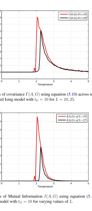
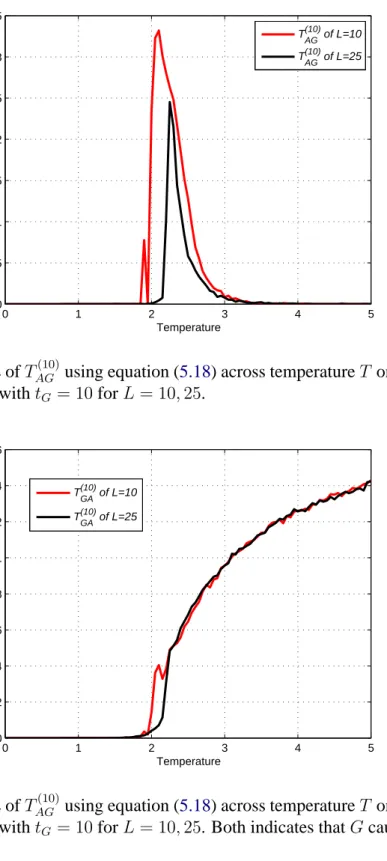
6.2 Measures on the amended Ising model . . . 97
6.2.1 Observables for verification of the critical point . . . 97
6.2.2 The influence of distance . . . 100
6.2.3 Measures onL= 25 . . . 103
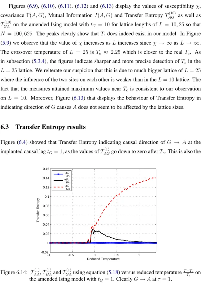
6.3 Transfer Entropy results. . . 106
6.3.1 Transfer Entropy as a causal lag indicator . . . 107
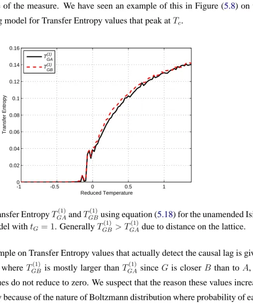
6.3.2 Discussions on the nature of Transfer Entropy . . . 109
7 A toy model 112 7.1 A simple model . . . 112
7.1.1 Probabilities on the simple model . . . 114
7.1.2 Transfer Entropy on the simple model . . . 117
7.2 The general model . . . 118
7.2.1 The relationship betweenΩandQ . . . 121
7.2.2 Transfer Entropy on the model . . . 123
7.2.3 Transfer Entropy for causal lag detection . . . 125
7.3 Cases of the general model . . . 130
7.3.1 Case 1:Ω = P(Zn−tZ = 1) . . . 131
7.3.2 Case 2:Ω = P(Zn−tZ 6= 1) . . . 133
7.3.3 Case 3:Ω = 12 . . . 134
7.3.4 Discussion . . . 135
8 Finite sampling effects and estimations 138 8.1 Simulation of the toy model . . . 138
8.1.1 Simulation ofns= 2 . . . 139
8.1.2 Simulation of Case3 . . . 141
8.1.3 Different cases of the general model . . . 143
8.2 The null model . . . 145
10
8.2.2 Mutual Information and covariance on the null model . . . 147
8.3 Correcting for finite sampling effects . . . 147
8.3.1 Surrogates for significant testing . . . 149
8.3.2 Effective and Corrected Transfer Entropy . . . 150
8.4 Estimation of Entropy . . . 152
8.4.1 Classical histogram (equidistant binning) . . . 152
8.4.2 Rankings and symbolic analysis . . . 154
8.4.3 Other nonparametric estimations . . . 155
8.4.4 Transfer Entropy estimators . . . 157
9 Application to EEG Data Sets 159 9.1 Visualizing the data . . . 160
9.1.1 Transfer Entropy on sine waves . . . 162
9.1.2 Stationarity and ergodicity . . . 165
9.2 Transfer Entropy between hemispheres of the brain . . . 166
9.2.1 Transfer Entropy of parietal cortices . . . 166
9.2.2 Transfer Entropy of the frontal cortices . . . 168
9.2.3 The interaction between frontal and parietal cortices . . . 171
9.3 Discussion. . . 174
9.3.1 Frontal cortices . . . 174
9.3.2 Causal lag detection . . . 175
10 Conclusion and Future Research 178 10.1 EEG data analysis . . . 179
10.1.1 What is causality of EEG data sets? . . . 179
10.2 The models and its potential . . . 181
10.2.1 Linking the model and data sets . . . 182
10.3 Information theoretic measures . . . 183
10.3.1 Variations of Transfer Entropy . . . 183
10.3.2 Generalized Mutual Information . . . 184
11
Chapter 1
The brain as a complex system
Statistical mechanics works towards understanding the macroscopic behaviour of a system from the microscopic interaction of its part. Lately the field has taken interest in complex systems, loosely defined as a system where the components self-organize into a critical state [6, 27, 53]. Criticality (the critical state) occurs when local distortions propagates throughout the entire system and observables are scale free [27, 53]. In this introductory chapter, we will first explain how the brain is essentially a complex system and how it is logical for it to operate near criticality. Then we look at the methods of analysing neuro data sets and why EEG data sets suits our purposes. After looking at some of the many different measures people have used on EEG data sets, we will most importantly explain our simplistic view of the brain and why we are looking for a measure that should essentially be nonlinear and be able to detect possible ‘causality’.
1.1
Complexity and the brain
Although there is no universally agreed upon definition of complex system, there are a few criteria that most will say define the system, mainly that it is composed of a large number of interacting components that give rise to emergent hierarchical structures and that the components typically change with time [54]. There is increasing belief among neurologists is that the brain is complex [20,43, 92]. In fact, it has been suggested that this wonderful brain of ours, could possibly be the most complex system of them all, due to its capability to
1.1 Complexity and the brain 12 represent the complex outer world to us humans [6]. Indeed, we are what we are perceived to be. A simple way to view the brain as a complex system is to imagine the neurons as individual components and the brain as a whole that emerges from cooperation of the neurons.
1.1.1
Complex systems and criticality
In other words, the brain is viewed as a system that exhibits complex behaviour where hundred billions of neurons self organize to function as one entity. However, some neu-rons seem to work together with one another more than others depending on the performed function [24, 92]. Consequently, it is believed that the brain can be divided into its func-tional parts [25,36]. Therefore, one could also consider the functional parts (encompassing certain areas of the brain) as the components that cooperate to become the brain as a whole. This is where a contradiction arises, on one hand the brain needs to be segregated for it to specialize and efficiently respond to specific stimulus (or lack of it) but on the other hand scientist have confirmed from many different sources and observations that virtually all perceptual or cognitive tasks are the end result of large scale and distributed activities, often times involving spatially disconnected area [25,24]. This integration versus segrega-tion issue is succinctly summarized in [92]. This apparent contradiction can be explained beautifully if we look at the brain as complex system. In order to further understand this currently prevalent paradigm about how the brain works we need to first understand criti-cality.
Criticality is the emergence of the components to work together as one. A familiar example will be the phase transition occurring when water evaporates into vapor. A phase transition with long range interactions (diverging correlation lengths) is critical. Basically in a complex system, criticality occurs when the system appears to act cooperatively as the result of individuals interactions [27, 53]. Therefore as a complex system, the brain is completely connected (acting cooperatively) and integrated at criticality as well as being segregated (acting individually or according to its functional speciality).
If a system is critical, there will be long range correlations as well as short range ones; in fact all scales of correlation should be present. Thus, theoretically the system will appear
Chapter 1. The brain as a complex system 13 identical no matter the scale at which we probe it, hence the term “scale free”. This self similar and scale free behaviour is fractal in nature which leads to the belief that a complex system is also fractal [27, 53]. This fact allows us to use scale free and self similarity as indicators of a system being in a critical state. The ability of certain data sets to appear self similar regardless of hierarchies and coarse graining is often taken to be an indication of criticality. However caution must be taken here since there can be other causes [104] for a system to be fractal.
1.1.2
The Ising model at phase transition
A system is critical in a sense that all members influence each other. In a complex system the critical state is established solely because of individual interactions [6, 27, 53] but an equilibrium system needs to be fine tuned to obtain this criticality. Perhaps the simplest example of an equilibrium system is the Ising model [27]. It displays emergent cooper-ative phenomenon (long range correlations) at its phase transition which is characterised by scale free behaviour. Therefore, the Ising model is critical at its phase transition. Only at this critical state, complex systems and equilibrium systems are said to exhibit similar behaviours [27,53], thus looking into this simple Ising model can help gain insight into the complexities of a the brain.
Briefly, the Ising model is a model comprised of sites on a lattice, where each site can only be in two possible states, either up (+1) or down (-1). In this thesis, we restrict the interaction of the sites to only its nearest neighbour (in two dimensions this will be nodes to the north, south, east and west). The effective interaction strength increases or decreases depending on temperature that effects the probability of the sites being in certain configura-tions. Amazingly, although only nearest neighbour interaction occurs, a specific site is able to influence other sites across the entire system at the critical temperature. The existence of this long range correlation at its phase transition, makes the model very interesting despite of its simplicity.
In fact, Fraiman et al. [38] compared the Ising model at criticality and the resting state of the brain obtained from functional magnetic resonance imaging (fMRI) data sets, and concluded that both the systems exhibit identical dynamics and statistical properties. They
1.1 Complexity and the brain 14 proposed that resting state (i.e the states when there are no explicit inputs or outputs) could be the default mode of the brain where certain areas are automatically activated during rest time and deactivated as soon as the slightest task is engaged upon. They even went further to suggest that the global changes in the brain (mood, attention etc) could be brought about the same way temperature drives the Ising model to criticality.
1.1.3
The brain operating near criticality
At first glance it looks like the brain must be critical since it has the capacity to allow communication between different parts of the brain at a speed that seems instantaneous. A critical system is highly susceptible to local distortion which resonates throughout the system. The brain seems to be doing exactly this when it switches between connections to figure out the appropriate responds to an external stimuli. Even when it is not stimulated it is perpetually changing [6, 20]. Moreover, if the brain was subcritical then only local correlations will occur and cooperative behaviour cannot be possible as the signals will die out. On the other hand, if the brain was supercritical there will be chaotic disorder as neurons will be firing and be massively activated all the time. Thus, it can be argued that the brain has to be critical for information to propagate and be comprehensible. There are even some scale free indicators found in the brain to support this hypothesis of criticality and fractal nature of the brain [25,34,36].
The idea that in order to be a dynamical system, the brain would have to operate near criticality was put forward by Turin in 1950 [104]. Being near criticality is very logical in terms of efficiency. Making use of local and global interaction appropriately as needed to balance out the integration and segregation as required is efficiency at its best. Brain scientists have confirmed that interactions in the brain are predominantly local [92]. Nev-ertheless, it does not work alone in its locality and needs to able to attain criticality very quickly. The brain connects and reconnects all the time according to its need and amazingly although the cortex is mainly excitory network it does not explosively propagate and still transmit information [24]. Thus it has to be near criticality. In fact Tagliazucchi et al. [97] claims to have evidence proving that in resting state, the brain spends most of its time near critical point where the dynamics are close to phase transition with long range correlations.
Chapter 1. The brain as a complex system 15 The main reason for this is that near the critical point, the system is anticipating criticality therefore a lot of different meta-stable states exist [38]. This makes the brain elastic and enhances the plasticity of the brain, to take the form of whatever state required.
One thing that we are very confident about is the fact that the brain handles loads of information. Thus some parts of the brain would be dependent on others at certain points in time. It is this flow of information and dependencies that we hope to understand a bit more of in order to contribute towards our understanding of the inner workings and complexities of the brain.
1.2
Peeking into the brain
The advances of technology have given us glimpses of what we hope to be the inner work-ings of the brain. Unfortunately making sense of these glimpses, is not an easy task to say the least. Adding to the difficulties is the fact that, on one hand it seems that different parts of the brain are activated at different times but on the other hand it appears almost like information is reaching all neurons at all times. Consequently, tracing the informa-tion flow in the brain will require high temporal resoluinforma-tion in order to capture split second changes. Electroencephalograph (EEG) may be able to do just that. On July 6, 1924 Hans Berger first used EEG to measure human brain waves [43, 84]. EEG is the recording of electrical activity along the scalp. The EEG can be defined roughly as the mean electrical activity of certain sites on the scalp [84]. The electrical activity is detected as the differ-ence in potential between two electrodes in a grounded system. With several electrodes on the scalp, an estimate map of the brain’s electrical charges can be constructed. This noninvasive technique is still the most widespread method used in laboratories [20].
Neuroimaging techniques are techniques used to visualize brain activity. The most popular of these techniques are functional magnetic resonance imaging (fMRI), positron emission tomography (PET) and single-photon emission computed tomography (SPECT) which assess metabolic correlates of neurons in blood flow, blood volume and oxygenation respectively [20]. The most prominent among those is the fMRI due to the prevalance of MRI scanners. This method which makes use of a magnet weighing several tonnes, depends on the magnetic moments of metal ions in our blood. fMRI makes use of the fact
1.2 Peeking into the brain 16 that the magnetic property of hemoglobin changes with presence and absence of oxygen. The information gathered by an fMRI scanner is usually processed to construct images of brain activities [20,43]. There are many interesting studies that have made use of data sets produced by fMRI [38,36,97].
1.2.1
EEG versus fMRI
The strength of fMRI lies in the spatial resolution. The easy-on-the-eye resulting images obtained from the MRI scans make it possible to detect cellular activity in structures that do not contribute to scalp EEG. A main technical drawback of the fMRI method is its slow temporal resolution [20]. EEG on the other hand has a very high temporal resolution but lower spatial resolution. EEG has come a long way since the time of Hans Berger but the general idea of recording electrical activity on the scalp remains. Fortunately for us the temporal resolution now is very high to the point where we could even possibly detect reactions at a neuronal level.
EEG and fMRI are both non-invasive procedures, however there are plenty of more-than-invasive experiments performed on the brains of animals including rats [12], cats [22] and monkeys [67]. In all of these experiments the neurons reacted in order of milliseconds. Therefore we believe that the human brain reacts similarly, that cooperative neuronal in-teractions are manifested in the order of milliseconds which can be detected by the EEG but not the fMRI. The temporal resolution is the most important reason we are interested in EEG data sets, especially when the brain appears to reorganize itself almost instanta-neously [20], in what appears to be the most effective information dissemination process in the universe. Additionally from a theoretical point of view, the high temporal resolution renders more data per second which leads to a much better probability estimate when one takes the average over time relative to the estimates that can be obtained from fMRI data sets.
Moreover, EEG technology has its advantages over the neuroimaging technique espe-cially in terms of portability, availability and at least 85 year history of investigation. MRI machines are typically huge and noisy enclosures which can sometimes intimidate whereas EEG involves wearing a string of electrodes on ones head. It is simply psychologically and
Chapter 1. The brain as a complex system 17 physically more convenient. Not to mention that it is also much cheaper than the fMRI. The simplicity and widespread usage of the EEG gives it the edge. It is much easier for a pianist for example to play the piano with some electrodes on his head then in an MRI scanner. Furthermore, the existence of smaller and more efficient EEG recording machines makes data acquisition less time consuming. In our case, EEG refers to the recording of the brain’s spontaneous electrical activity over a short period of time, as recorded from eight electrodes placed on the scalp.
1.2.2
Details of the EEG data set
Thanks to the team of EEG experts led by Bj¨orn Cr¨uts at Biometrisch Centrum (BMC) [1], that make their own EEG recording devices, we have EEG data sets from possibly the most up-to-date machine. Bj¨orn’s team have kindly shared some of their data sets and also gave very valuable advice with regards of the outcome of the analysis. The team is continuously working with clinicians all over the Netherlands (and currently expanding to some parts of Germany) in using EEG in psychological treatments and providing EEG machinery as well as training to the psychologist. The team strive to use the best quality materials for their machines and they are constantly trying to improve the efficiency and design of their EEG machines. The data sets provided to us were recorded at 250Hz (4 millisecond intervals) with a resolution smaller than 0.1 millivolts. These data sets motivated us to think about how the brain operates.
1.3
Measures on EEG data sets
In order to make sense of all the acquired EEG data obtained using these technologically advance machines, a certain type of measure must be used to quantify these data. There are many to choose from. The ever popular correlation deserves our attention first. But before that, some definitions that will be adopted throughout the thesis.
1.3 Measures on EEG data sets 18
1.3.1
Probability and Expectation
We shall defineP as the probability. The most common way we shall useP is in terms of expressing variables and its different possible values, that we shall call states. For example, define two variablesX andY that can be in statesx ∈ X andx ∈ Y respectively. X is the state space (set of all possible states) ofX andY is the state space ofY. P(X =x) =
pX(x) is the probability of X being in state x. P(X = x, Y = y) = pXY(x, y) is the
joint probability ofX being in statexandY being in stateysimultaneously. With regards to the conditional probability, we shall use P(X = x|Y = y) = pX|Y(x|y)to denote the
probability ofXbeing in statexgiven thatY is in statey. These terms can be generalized for relationship between many variables.
Thus if X ∼ pX(x) [X has distribution pX(x)] as we have defined above, then the
expected value of random variablef(X)is written [29] as
EpX(x)[f(X)] =
X
x∈X
pX(x)f(x) =E[f(X)]. (1.1)
The last term on the right hand side (RHS) will be used when the probability distribution is understood from the context. Moreover, sometimes we shall take the liberty of simply usingP(X) = P(X =x),P(X|Y) = P(X =x|Y =y)and so on, especially when using P in tandem with expectationE and when the context is clearly understood. However this is not to be confused with the general usage ofP as the probability of an event. For example ifA ={Xdoes not change}thenP(A) =P(Xdoes not change)is the probability thatX does not change which is equal to the probability of eventA.
1.3.2
Covariance and Correlation
The most common measure on neuro data sets (or any kind of data in statistical mechanics for that matter) is correlation. Correlation in a general sense of the word is commonly used to refer to the mutual relationship or connection between two or more things. Even when discussing the relationship between variables, correlation is often referred to in the context of whether or not there exist co-relation between them. In statistical mechanics, correlation often refers to a measure of mutual order existing between variables [109].
Chapter 1. The brain as a complex system 19 Unfortunately (and this is where it sometimes get confusing) this is usually done using the covariance measure. Recall the two variablesX andY previously defined. Given that the joint probability ispXY(x, y), the covariance ofX andY is defined as
Γ(X, Y) = E[XY]−E[X]E[Y] =X x∈X X y∈Y xypXY(x, y)− X x∈X xpX(x) X y∈Y ypY(y). (1.2)
In some literature this quantity is known as the correlation, we cautiously use the term covariance here to distinguish it from the statistical correlation [36,109],
ρ(X, Y) = Γ(X, Y)
σ(X)σ(Y) =
E[XY]−E[X]E[Y]
σ(X)σ(Y) (1.3)
where σ(X) is the standard deviation of X (note that ρ is undefined when X or Y is constant sinceσ(X) = 0). The variablesX andY are said to be ‘uncorrelated’ or linearly independent whenΓ(X, Y) = 0.
LetXτ be the variable X that is shifted byτ time steps. For example, ifX is in state 1at time step1, state2at time step2and so on. DenoteXnfor value ofX at time stepn.
Xτ is the variable Xshiftedτ time steps so that the values ofXτ areτ time step ahead of
X i.e. Xτ
n =Xn+τ. The cross correlation is used to measure correlation across time step
such that
ρ(Y, Xτ) = E[Y X
τ]−E[Y]E[Xτ]
σ(Y)σ(Xτ) . (1.4)
Similarly, cross covariance is defined as Γ(Y, Xτ). Autocorrelation is simply the
corre-lation of a variable with a time shifted version of itself (hence the word auto) such that ρ(X, Xτ). Correlation is widely used in measuring quantities in many fields including
neuroscience. It is extensively used on EEG data sets [5].
1.3.3
Other measures
Measures can be used in time domain or in frequency domain. The previous measures were mentioned in the context of time domain. There are many other measures that requires the
1.4 How we humans view the brain 20 EEG data set to be in the frequency domain since there are strong reasons to believe that fre-quencies are important on EEG data sets. The most basic one would be coherence [44,18], which is simply correlation as a function of frequencies allowing spatial correlation to be studied between different frequencies. For a review on how coherence have been used on EEG see [84]. More recently, popular measures for the frequency domain in neuroscience include Partial Directed Coherence (PDC) and Direct Transfer Function (DTF) by Taka-hashi et al. [99].
However, in this thesis we only discuss measures in the time domain. Most of our find-ings are similarly applicable to the frequency domain by simply replacing the probability density function with the spectral density function. We will be focusing on entropy based measures originating from information theory. The use of measures from information the-ory is aptly appropriate considering that it has been said to be a natural tool set to use on the brain [98] due to the vast amount of information processed.
1.4
How we humans view the brain
The way we humans picture the brain is constantly evolving. The ancient Egyptians appar-ently did not consider the brain to be important, thus taking it out and throwing it away from their dead ones during mummification. The ancient Greeks are the ones usually credited to be the first to think that the brain was important. The idea that the mind and matter is con-nected, is known to be propounded by Pythagoras who thought that the mind is somehow attuned to the laws of mathematics. Whether or not this happened in the brain was prob-ably not important to him. However, Hippocrates who came decades later argued that the brain is the most important organ for sensation, thought, emotion and cognition [20]. Fur-thermore, he divided the brain into four humours responsible for different temperaments. Recent developments in technology and complexity science has resulted in paradigm shifts in terms of how we look at the brain, most of the neuroscientists are now of the view that the whole brain is also integrated in addition to having different functionalities [92].
Chapter 1. The brain as a complex system 21
1.4.1
Simplistic view of the brain
The idea that there exist dedicated parts of the brain for certain functionalities persisted. In the current literature it is known as functional segregation which refers to specialized neurons responding to specific input features. There are even claims that every cognitive act has its specific assembly that causes its emergence [24]. Its counterpart, the functional integration on the other hand, refers to the establishment of a statistical relationship be-tween different and distant cell populations which may ironically degrade specialization [92]. From a very machine-like point of view the brain performs two very important and almost contradictory actions. The first is the need to extract the information from the input (stimulus) that it receives. This is where segregation is needed. At the same time (or within a few milliseconds) it has to make sense and then react to the stimulus accordingly. And this is where integration comes into play. Looking at the brain as a complex system that is constantly near criticality brings these two functions together.
Nonlinearity is fundamental in any complex system. By definition, the emergence and criticality expected in a complex system is a nonlinear phenomenon. The fact that we be-lieve the brain is operating near criticality thus being crucially nonlinear encouraged us to look for measures that can capture nonlinearities. Nonlinear relationships are prevalent in the brain, small inputs can stimulate large outputs or sometimes none at all [20]. The func-tional integration (connectivity) of the brain which is defined as the connections between distant groups of cells are commonly established using temporal correlations (cross corre-lation by our definition) or temporal covariance [92]. We are hoping to look at things in a more nonlinear manner. Therefore, in our simplistic approach to understanding the brain, nonlinearity will be one of the main issues.
The idea of functional segregation can sometimes be explained in terms of certain spe-cific parts of the brain controlling certain spespe-cific functions. However, these controlling areas are not the only ones that are active during the operation of the task and sometimes the communicating areas are not even spatially connected [98]. Therefore, there must be some form of communication between the areas especially when reacting to external inputs. The communication links exist mostly as a series of action potentials forming a connec-tion. The length of this connection in a single human brain is said to be between100,000
1.4 How we humans view the brain 22 to10,000,000kilometres [92]. This emphasizes the importance of communication in the brain in order for it to function as a directed network. The key word here is directed, having a starting point and an end point. The very definition of the functional integration was to establish a sort of temporal relationship between groups of cells and therefore establishing ‘causal’ (directed) link between these groups. Therefore, the second element that we wish to incorporate in our simplistic model of the brain is a type of ‘causality’.
Chapter Summary
We have first explored how the brain could be the very definition of a complex system and how technology can help us understand it better. Subsequently, we explained our interest in EEG data sets and went through some basic introduction on how people go about measuring it. The very nature of the brain where there is bound to be ‘causal’ connections in a very nonlinear environment of a complex system points out the need for a measure that can incorporate both nonlinearity and ‘causality’. We start by examining how to capture the nonlinearity and this is where Mutual Information comes into the picture.
23
Chapter 2
Mutual Information as a nonlinear
measure
To capture the nonlinearities of the brain, we need a nonlinear measure. The Mutual In-formation which is based on inIn-formation theoretic entropy introduced by Shannon in his seminal paper [91] seems to fit this description. Firstly, we define entropy and its unique-ness in defining uncertainties. Consequently we define Mutual Information and Kullback Leibner measure as function of probabilities. We discuss some of the common properties of these measures. In terms of independence, we show how Mutual Information is tailor made to capture the very definition of independence in contrast to covariance which is es-sentially defined to capture linear independence. Lastly, we will take a brief look at some applications of the Mutual Information including possible ‘causality’ detection.
2.1
Entropy
In statistical mechanics, entropy arises as a measure of uncertainties and disorganization in a physical system. Information theory deals with entropy in a slightly different man-ner as it focuses on the quantification of information. Mutual Information is an entropy based measure widely used in information theory. In order to understand Mutual Informa-tion, we need to understand entropy. Entropy was first coined in 1865 by Rudolf Julius Emmanuel Clausius [59] in reference to thermodynamics. However in 1948, Shannon
de-2.1 Entropy 24 fined a slightly different kind of entropy in terms of measurable dynamics and information theory. It was reported that he contemplated calling it information or uncertainty but was convinced by John Von Neumann to call it entropy for two reasons. The first was that entropy is the uncertainty function of statistical mechanics and secondly according to Neu-mann, to call it entropy will be advantageous in debates since nobody knows what entropy really is [59].
On a more general level, the field of complex networks is still looking for a good quan-tifier of complexity and there seems to be a great need for a new theory of information of complex networks [3]. One way to tackle this issue is to import the key concepts of information theory that has quantification of information as the main focus where entropy based measures such as Mutual Information plays a key role. Being able to evaluate the information transfer of a complex system is one of the main outstanding problems in the statistical mechanics of the complex systems.
2.1.1
The definition of entropy
Shannon [91] defined entropy as the functionH(p1, p2, ..., pn)for probabilitiesp1, p2, ..., pn,
H(p1, p2, ..., pn) =−k n X
i=1
pilog pi (2.1)
where k > 0 is a constant and the log is to the base 2. The aim was to measure the un-certainty of the outcome of a certain variable given the probabilities. H was chosen to represent uncertainty due to it being the only the solution to certain properties that are outlined to ‘measure’ uncertainty [91] . Khinchin [58] came up with a more mathemati-cally rigorous proof for uniqueness ofHfor the chosen properties. Before outlining these properties in subsection (2.1.2), we explain more aboutH.
Whenp1, p2, ..., pnare the probabilities of discrete random variableX we write
H(X) =H(p1, p2, ..., pn) = − n X
i=1
pilog pi (2.2)
Chapter 2. Mutual Information as a nonlinear measure 25 X is not the argument of the functionH but it is the random variable the entropy of which we are trying to measure. For example, say we have a random variableXwith probabilities p1 = P(X = 1) = 13, p2 = P(X = 2) = 12 andp3 = P(X = 3) = 16, then the entropy
would be H(X) = −1 3 log 1 3− 1 2 log 1 2− 1 6log 1 6.
Entropy does not actually depend on the values taken by random variable X but only its probabilities. This entropy definition is also prominent in measure theory and ergodic theory [52,59].
More formally, define two random variablesXandY that have probabilitypX(x), x∈
X andpY(y), y ∈ Y, respectively.X is the state space (set of all states) ofX andY is the
state space ofY. Their respective entropies [29] are
H(X) = −X x∈X pX(x)log pX(x) (2.3a) and H(Y) = −X y∈Y pY(y)log pY(y). (2.3b)
We will use the convention 0 log 0 = 0 which is easily justified by continuity since x log(x)→0asx→0and log to the basee. In terms ofE, we have
H(X) =−X
x∈X
pX(x)log pX(x) = EpX(x)[−log pX(x)] =E[−log P(X)]. (2.4)
Therefore, the entropy ofX can also be interpreted as the expected value of−log pX(x)
when X ∼ pX(x) [29]. Recall that pX(x) = P(X = x) and E is the expectation as
2.1 Entropy 26
2.1.2
The uniqueness of entropy
When more than one variable is involved, joint and conditional entropy can be defined [29,52]. The joint entropy ofX andY is defined as
H(X, Y) = −X
x∈X
X
y∈Y
pXY(x, y)log pXY(x, y) =E[−log P(X, Y)]. (2.5)
DefineH(Y|X = x) = −Py∈YpY|X(y|x)log pY|X(y|x), so that the conditional entropy
can be written as H(Y|X) = X x∈X pX(x)H(Y|X =x) = − X x∈X pX(x) X y∈Y pY|X(y|x)log pY|X(y|x) =−X x∈X X y∈Y
pXY(x, y)log pY|X(y|x) =EpXY(x,y)[−log P(Y|X)] (2.6)
where we have substitutedpY|X(y|x)pX(x) =pXY(x, y).
The Uniqueness of Entropy was later on proven in mathematically rigorous way by Khinchin [58] whenHhas these properties:
1. Givennpossibilities,H is maximum whenpX(x) = 1n for∀x∈ X.
2. The chain rule:H(X, Y) =H(X) +H(Y|X).
3. Adding an impossible event i.e a zero probability event does not change the value of H:H(p1, p2, ..., pn,0) = H(p1, p2, ..., pn).
As a side note, we would like to point out a trivial point that will make working with expectations much simpler. For any function ofX,f(X)with distribution functionpX(x),
we have that EpX(x)[f(X)] = X x∈X pX(x)f(x) = X x∈X X y∈Y pXY(x, y)f(x) = EpXY(x,y)[f(X)], (2.7)
where we made use of the joint probability property Py∈YpXY(x, y) = pX(x).
Chapter 2. Mutual Information as a nonlinear measure 27 P(X, Y) =P(X)P(Y|X)into equation (2.5) as follows
H(X) +H(Y|X) = EpX(x)[−log P(X)] +EpXY(x,y)[−log P(Y|X)]
=EpXY(x,y)[−logP(X)P(Y|X)] =EpXY(x,y)[−log P(X, Y)]
=H(X, Y). (2.8)
This rule links joint and conditional entropy. By symmetry we also have H(X, Y) =
H(Y) +H(X|Y). It is possible to include more variables in the definition of joint and conditional entropy where the definitions can also be linked using the chain rule. If we define a new random variableZin a similar manner, using the equality from Bayes theorem pZ(z)pXY|Z(x, y|z) =pXY Z(x, y, z)and the definition of the conditional entropy, we get
H(X, Y|Z) = X z∈Z pZ(z)H(X, Y|Z =z) =−X z∈Z pZ(z) X x∈X X y∈Y pXY|Z(x, y|z)log pXY|Z(x, y|z) =−X x∈X X y∈Y X z∈Z pXY Z(x, y, z)log pXY|Z(x, y|z) =EpXY Z(x,y,z) [−log P(X, Y|Z)]. (2.9)
And by substitutingpY Z(y, z)pX|Y Z(x|y, z) =pXY Z(x, y, z), we obtain
H(X|Y, Z) =X y∈Y X z∈Z pY Z(y, z)H(X|Y =y, Z =z) =−X y∈Y X z∈Z pY Z(y, z) X x∈X pX|Y Z(x|y, z)log pX|Y Z(x|y, z) =−X x∈X X y∈Y X z∈Z pXY Z(x, y, z)log pX|Y Z(x|y, z) =EpXY Z(x,y,z)[−log P(X|Y, Z)]. (2.10)
It is clear that by simple manipulation of the probabilities using Bayes theorem we can get relations between conditional entropies. For example, using Bayes theorem to manipulate
2.2 Mutual Information and Relative Entropy 28 the probabilities we get
pXY|Z(x, y|z) = pXY Z(x, y, z) pZ(z) = pY|XZ(y|x, z)pXZ(x, z) pZ(z) =pY|XZ(y|x, z)pX|Z(x|z),
so that the entropy of X andY conditioned onZ is equal to entropy ofY conditioned on XandZ plus the entropy ofXconditioned onZ, i.e.
H(X, Y|Z) = H(Y|X, Z) +H(X|Z). (2.11) We are now prepared to define Mutual Information.
2.2
Mutual Information and Relative Entropy
For the same random variablesX andY, the Mutual Information [29,60,61,64,73,103] is defined as
I(X, Y) = H(X)−H(X|Y)
=EpX(x)[−log P(X)]−EpXY(x,y)[−log P(X|Y)]
=−E[log P(X)] +EpXY(x,y) logP(X, Y) P(Y) =EpXY(x,y) log P(X, Y) P(X)P(Y) =X x∈X X y∈Y pXY(x, y)log pXY(x, y) pX(x)pY(y) . (2.12)
I can be interpreted as the amount of informationY provides about X since it measures the difference between the uncertainty of X and the the uncertainty of X given Y. The relationship can also be viewed in a set theoretic setting as in Figure (2.1). If we define H(X)andH(Y)as sets, then we have thatI(X, Y) = H(X)∩H(Y)and thatH(X, Y) =
H(X)∪H(Y). The conditional entropies are given byH(X|Y) = H(X)\I(X, Y)and H(Y|X) =H(Y)\I(X, Y). From the definition and the Venn diagram we can see thatIis
Chapter 2. Mutual Information as a nonlinear measure 29
Figure 2.1: Venn diagram depicting relationship betweenIandH
symmetric so that the information thatY gives aboutXis the same amount of information Xgives aboutY. The symmetry of Mutual Information can be shown using the chain rule in equation (2.8).
I(X, Y) =H(X)−H(X|Y) =H(X)−[H(X, Y)−H(Y)]
=H(Y)−[H(X, Y)−H(X)] =H(Y)−H(Y|X) =I(Y, X). (2.13) Note thatI(X, X) = H(X)−H(X|X) =H(X)sinceH(X|X)is obviously zero. There-foreH is a special case ofI.
2.2.1
Relative Entropy and conditional Mutual Information
Another interesting way of interpreting Mutual Information is through relative entropy. Relative entropy or Kullback Leibner (KL) distance [29, 52,63] between two distribution functionsf(x)andq(x)is defined as
D(f||q) =X x∈X f(x)log f(x) q(x) =Ef log f(X) q(X) ,
where we take 0log 0
q = 0 and 0log
f
0 = ∞. D can be seen as a measure of distance
between distributions. However it should be pointed out that it is not a true metric distance because it is not symmetric and does not satisfy the triangle inequality. Despite that, it is often helpful to think ofD as the distance between f and q, because it seeks to quantify the difference between these two distributions and D = 0 when f(x) = q(x). If we let
2.2 Mutual Information and Relative Entropy 30 f(x) = pXY(x, y)andq(x) =pX(x)pY(y)then we get that
D(pXY(x, y)||pX(x)pY(y)) =EpXY(x,y) log P(X, Y) P(X)P(Y) =I(X, Y). (2.14)
It appears thatI is just the special case ofDwhere f is the joint distribution andq is the product distribution. Using this logic, we can interpretI as measuring how ‘far’ the joint distribution is from the product distribution.
Analogous to entropy, the definition of Mutual Information can be extended to include a third random variable Z in the form of conditional Mutual Information [29, 52] which can be written as I(X, Y|Z) = H(X|Z)−H(X|Y, Z) =E[−log p(X|Z)]−E[−log p(X|Y, Z)] =E log p(X|Y, Z) p(X|Z) =E log p(X, Y, Z)p(Z) p(Y, Z)p(X, Z) =EpXY Z(x,y,z) log P(X, Y|Z) P(Y|Z)P(X|Z) , (2.15)
where one can clearly see that the only difference with the Mutual Information definition in equation (2.12) is that the probabilities are conditioned onZ. Conditional Mutual Infor-mation can be interpreted as the amount of inforInfor-mationXprovides aboutY (or vice versa) given thatZ is known.
2.2.2
Properties of Entropy, Relative Entropy and Mutual Information
EntropyH is a specific case of Mutual InformationI. Mutual InformationI is a specific case of relative entropy D. So all properties of D extends to I and all properties of I extends to H. This does not apply in the other direction. One prevailing property for all three quantities is non-negativity. This can be proven using Jensen’s Inequality [29, 108] which states that ifgis a convex function thenE[g(X)]≥g(E[X]). And ifg is a concave function thenE[g(X)] ≤g(E[X]). Letf(x)andq(x)be distribution functions, we claim thatD(f||q)≥0andD(f||q) = 0if and only iff(x) = q(x)for anyx. Forf(x), q(x)>0Chapter 2. Mutual Information as a nonlinear measure 31 we have that −D(p||q) =−Ef(x) logf(X) q(X) =Ef(x) logq(X) f(X) ≤log Ef(x) q(X) f(X) =logX x f(x)q(x) f(x) =log X x q(x) =log1 = 0
where the inequality follows from Jensen’s inequality since the functionlog(x)is a concave function ofx. Thus I(X, Y) = D(pXY(x, y)||pX(x)pY(y)) ≥ 0andI(X, Y) = 0 if and
only ifpXY(x, y) =pX(x)pY(y). MoreoverH(X) =I(X, X)≥0andH = 0only when
Xis constant [29]. However it must be pointed out that
I(X, Y|Z) =EpXY Z(x,y,z) log P(X, Y|Z) P(X|Z)P(Y|Z) 6 =EpXY|Z(x,y|z) log P(X, Y|Z) P(X|Z)P(Y|Z) =D(pXY|Z(x, y|z)||pX|Z(x|z)pY|Z(y|z)),
and that D ≥ 0 does not necessarily implies that the conditional Mutual Information I(X, Y|Z)≥0. HoweverI(X, Y|Z)≥0can also be proven using Jensen’s inequality.
I(X, Y|Z) = EpXY Z(x,y,z) log P(X, Y|Z) P(X|Z)P(Y|Z) =EpXY Z(x,y,z) −logP(X, Z)P(Y, Z) P(X, Y, Z)P(Z) ≥ −log EpXY Z(x,y,z) P(X, Z)P(Y, Z) P(X, Y, Z)P(Z) =−logX x∈X X y∈Y X z∈Z pXY Z(x, y, z) pXZ(x, z)pY Z(y, z) pXY Z(x, y, z)pZ(z) =−logX y∈Y X z∈Z pY Z(y, z) pZ(z) X x∈X pXZ(x, z) = −log X y∈Y X z∈Z pY Z(y, z) pZ(z) pZ(z) =−logX y∈Y X z∈Z pY Z(y, z) =−log X z∈Z pZ(z) =−log 1 = 0.
One property of I not possessed by D is symmetry. Generally, D is not symmetric sinceD(p||q) = Eplogqp((XX)) 6= Eqlogqp((XX)) = D(q||p). I however, is symmetric because of
2.3 Mutual Information versus covariance 32 equation (2.13). Joint entropyH(X, Y)is symmetric since we get that
H(X, Y) =EpXY(x,y)[−log P(X, Y)] =H(X) +H(Y|X)
=H(Y) +H(X|Y) =H(Y, X).
On the other hand, conditioning reduces entropy hence distorting the symmetry i.e
H(X|Y) = −EpXY(x,y)[log P(X|Y)] =H(X, Y)−H(Y)≤H(X),
H(Y|X) = −EpXY(x,y)[log P(Y|X)] =H(X, Y)−H(X)≤H(Y),
so thatH(X|Y) 6=H(Y|X)in general. It is the same case forI, generallyI(X, Y|Z)6=
I(X, Z|X) 6= I(Y, Z|X)since the probabilities could be different although we obviously still haveI(X, Y|Z) = I(Y, X|Z).
2.3
Mutual Information versus covariance
One feature of Mutual Information is that it enables quantification of relationship between symbolic sequences [64]. This is due to the fact that Mutual Information only depends on probabilities rather than the values of the variable itself, consequently the variable does not have to be a number. It is pointed out that, in this way Mutual Information is somewhat more flexible than covariance (and correlation) function since it does require the variable to be a number. In a similar sense we can get relationship between blocks or group of nodes on the brain since all we need are the probabilities and not the values of the nodes itself. This could be very useful in identifying any scale free features of the brain to support the claim in [36]. However the most important difference is in terms of linearity and independence.
2.3.1
Comparing independence
The variablesX andY are said to be linearly independent of each other if
X x∈X X y∈Y xypXY(x, y) = X x∈X xpX(x) X y∈Y ypY(y). (2.16)
Chapter 2. Mutual Information as a nonlinear measure 33 It can easily be seen that the covariance and correlation is defined to capture linear inde-pendence. Recall the definition of covariance from equation (1.2) so that
Γ(X, Y) =E[XY]−E[X]E[Y] = 0 ⇒ E[XY] =E[X]E[Y] ⇒X x∈X X y∈Y xypXY(x, y) = X x∈X xpX(x) X y∈Y ypY(y) (2.17)
where the last line is the very definition of linear independence. Therefore E[XY] =
E[X]E[Y]implies thatXandY are linearly independent.
It is well known that two variables X andY are independent if and only if their joint distribution equals their product distribution [108] such that
pXY(x, y) = pX(x)pY(y)∀x∈ X, y ∈ Y. (2.18)
It is a well known fact in statistics that uncorrelated-ness (linear independence) does not imply (general) independence but independence implies uncorrelated-ness [46]. Anything that is independent would of course be linearly independent by default. Recall from equa-tion (2.14) that when pXY(x, y) = pX(x)pY(y) i.e when theX and Y are independent,
we have that I = 0. We have seen that I can be interpreted as measuring how ‘far’ the joint distribution is from the product distribution (which is the joint distribution when X andY are independent). In other words Mutual Information seeks to measure how depen-dent these two variables are on each other. One can see this from the definition of Mutual Information in equation (2.12) which renders
I(X, Y) = E log P(X, Y) P(Y)P(X) =E[log P(X, Y)−log P(X)P(Y)] = 0 ⇒ E[log P(X, Y)] =E[log P(X)P(Y)]. (2.19) Consequently it is logical to expect that, Mutual Information has the potential to provide us with insights that have not been obtained using covariance before. The direct approxima-tion approach should give us a clear indicaapproxima-tion of independence given that the probabilities
2.3 Mutual Information versus covariance 34 are accurately estimated. Moreover, even ifX and Y are not independent of each other, one could have
pXY|Z(x, y|z) = pX|Z(x|z)pY|Z(y|z)∀x, y, z
so that variablesX andY are said to be conditionally independent on variable Z. There-fore, ifX andY are conditionally independent onZ, we get thatI(X, Y|Z) = 0.
2.3.2
An illustrative example
The discussion on independence indicates thatΓ = 0; I = 0butI = 0 ⇒Γ = 0. This is demonstrated in [64] which starts off with a binary sequence where the numerical values ofXandY can only be either 0 or 1. In this case, we can find a relationship between these two functions and linear dependence would lead to general dependence. Therefore we have
thatΓ = 0 ⇔ I = 0for binary sequences.
Let p(α) and p(α, β) be the probability and joint probability for α, β ∈ {0,1}. The covariance in equation (1.2) becomes
Γ(X, Y) = E[XY]−E[X]E[Y] = p(1,1)−p(1)2, (2.20) so that we can write the probabilities in terms of Γ = Γ(X, Y). Using the property of joint probabilityPβp(α, β) = p(α)and imposingp(α, β) = p(β, α), we get thatp(1)−
p(1,1) = p(0)−p(0,0).Moreover, taking into accountp(1) +p(0) = 1(the normalizing condition for probabilities) we obtain
p(1,1) = Γ +p(1)2, (2.21a)
p(0,0) = Γ +p(0)2, (2.21b)
p(0,1) =p(1,0) = −Γ +p(0)p(1). (2.21c) The probabilities can be used to obtain the Mutual Information formula using equation
Chapter 2. Mutual Information as a nonlinear measure 35 (2.12) so that I(X, Y) =X α X β p(α, β)log p(α, β) p(α)p(β) =Γ log 1 + p(1)Γ2 1 + p(0)Γ2 Γ p(0)p(1) 2 +p(1) 2log 1 + Γ p(1)2 +p(0)2log 1 + Γ p(0)2 −2p(0)p(1)log 1 + Γ p(0)p(1) . (2.22)
This equation ties in with the fact that the lower bounds on Mutual InformationI for any kind of sequence has been proven to be dependent on the covariance Γand the marginal probabilities [37]. An approximation when the terms p(α)Γp(β) are small gives
I ≈Γ 2 2 1 p(1)2 + 1 p(0)2 + 2 p(0)p(1) = 1 2 Γ p(0)p(1) 2 . (2.23)
This illustrates thatI decays to zero at a faster rate than the correspondingΓ.
By settingα, β ∈ {0,1,2}, we get ternary sequences. To obtain a relationship between IandΓusing similar methods and constraints does not seem possible for ternary sequences. However, settingΓ = 0in equation (1.2) with current values ofX andY renders
Γ =E[XY]−E[X]E[Y] (2.24)
=p(1,1) + 2p(1,2) + 2p(2,1) + 4p(2,2)−(p(1) + 2p(2))2 = 0
and using this as an additional constraint, gives us probabilities to put in I to get values ofI corresponding toΓ = 0. In [64], some non-negative values for the probabilities were randomly chosen and this made clear that there are values for which Γ = 0 but I 6= 0. ThereforeΓ = 0 ; I = 0for ternary sequences in general. This demonstrates that the Mutual Information function is capable of capturing the nonlinear dependencies that the covariance might have missed.
2.4 Various applications of Mutual Information 36
2.4
Various applications of Mutual Information
Just like correlation, Mutual Information has also been defined and redefined to serve different purposes. The most natural extension is to insert an element of time and use the Mutual Information with its time shifted counterpart ala cross correlation in equation (1.4) such that I(X, Yτ) = H(X)− H(X|Yτ) where Yτ denotes a variable Y which
has been shifted by time τ. This value is known as pairwise cross Mutual Information [40] or time delayed Mutual Information [57, 89]. Mutual Information applied to its time shifted version is sometimes referred to as auto Mutual Information [2, 55, 56] such that I(X, Xτ) =H(X)−H(X|Xτ)whereXτ is the variableXthat is shifted byτ.
Some go even further by defining the persistent Mutual Information of a variable (some-times know as Mutual Information between past and future) which is the Mutual Informa-tion of the past history of a variable and it’s evoluInforma-tion later in the future [8]. Analytical works has been done on continuous Mutual Information for stochastic differential equa-tions on Gaussian cases where Mutual Information has been expressed as the mean square estimation error [7, 32,33]. Mutual Information have also been applied on the frequency domain [18] and is said to be better than coherence.
2.4.1
Quantifying transitions
Aiming to predict the future of evolving dynamical systems from the past using observed historical data, [8] uses the persistent Mutual Information on the logistic map and con-cluded that the measure succeeded in detecting different types of associated cascades of banded chaos in addition to period doubling. This is an example of how Mutual Informa-tion is utilized to quantify underlying transiInforma-tion in dynamical systems.
In [73], it is claimed that the Mutual Information is able to detect the phase transition occurring in a two dimensional Ising model. This claim has been corroborated on different systems on a few occasions. On the Viscek model of self propelled particles for example, [105] has claimed that Mutual Information is a sensitive indicator and phase transition locator. Furthermore, [105] claims that on this particular model, the Mutual Information works even better than susceptibility even when only partial observations are available. Drawing parallels between market crashes and phase transition under the assumption that
Chapter 2. Mutual Information as a nonlinear measure 37 collective pricing behaviour of the financial market works the like a complex systems, [47] claims that Mutual Information indicates the transition from random to collective behavior on the data sets.
2.4.2
Clustering and hierarchy detection
There are strong indicators that there exist hierarchies in the brain [20]. The grouping property of Mutual Information could provide a natural way for application in clustering algorithms. For this purpose, one could adopt the definition in [61] such that
M I(X, Y, Z) =H(X) +H(Y) +H(Z)−H(X, Y, Z)
is defined for random variables X, Y, Z as utilized before. This representation is useful since one could make use of the grouping property of Mutual Information so that
M I(X, Y, Z) = I(X, Y) +I((X, Y), Z),
whereI((X, Y), Z) =I(X, Z) +I(Y, Z|X)[29,61]. If we again define everything in set theoretic terms like in Figure (2.1) and consider H(X), H(Y) and H(Z)as sets so that I(X, Y) =H(X)∩H(Y),I(Y, Z) =H(Y)∩H(Z)andI(X, Z) =H(X)∩H(Z),then
M I(X, Y, Z) =I(X, Y)∪I(Y, Z)∪I(X, Z) (2.25a) and
I((X, Y), Z) = I(X, Z)∪I(Y, Z). (2.25b) We can clearly see from Figure (2.2) that
2.4 Various applications of Mutual Information 38
Figure 2.2: M I(X, Y, Z),H(X),H(Y)andH(Z)
These equalities can be generalized into
M I(X1, X2,∙ ∙ ∙ , Xn) = n X i=1 H(Xi)−H(X1, X2,∙ ∙ ∙ , Xn) I((X1, X2,∙ ∙ ∙ , Xn−1), Xn) = n X i=1 I(Xi, Xn|X1,∙ ∙ ∙ , Xi−1)
whereH(X1, X2,∙ ∙ ∙ , Xn) = Pni=1H(Xi|X1,∙ ∙ ∙ , Xi−1)is the generalization [29] of the
chain rule on entropy that we have defined before. Therefore Mutual Information could also be used as the proximity measure in a clustering algorithm, where the equations can be used recursively as a clustering tool. This have been done in [61] electrocardiogram (ECG) data. Examples of Mutual Information used for clustering and classification of EEG data are given in [56,2,55]. Other applications of Mutual Information based clustering can be seen in [21,4].
2.4.3
Detecting causality
The earliest criticism of ‘causality’ based test is that correlation is not equal to ‘causal-ity’ due to its symmetry [46]. Correlation and Mutual Information gives no indication of the direction of the relationship. Coming back to our aim of capturing both nonlinear-ity and ‘causalnonlinear-ity’, it would be great if Mutual Information is able to quantify ‘causalnonlinear-ity’. Therefore one would logically conclude that inserting an element of time into conditional Mutual Information will be more suitable for ‘causality’ detection. It so happens that there is a value called Transfer Entropy [89] that is said to be able to do just that. This value is
Chapter 2. Mutual Information as a nonlinear measure 39 simply an extension of the conditional Mutual Information where the conditional Mutual Information is utilized but now with its time shifted counterpart.
Consider the time shifted variable as in equation (1.4) and letX1be the variableXthat
is shifted by1(so that the values ofX1 always comes beforeX). Recall the definition of
conditional Mutual Information from equation (2.15) and let X = X1 andZ = X in the
definition so that
I(X, Y|Z) = H(X|Z)−H(X|Y, Z) (2.27)
=H(X1|X)−H(X1|Y, X) =I(X1, Y|X) = TY→X.
This is a simple example of Transfer EntropyTY→X as described by [89]. The idea is that,
ifY causesXat time lagτ = 1, thenI(X1, Y|X)will be large since a lot the uncertainties
ofX will be caused byY and the termH(X1|Y, X)will be much smaller thanH(X1|X).
However, before we delve further into how exactly the Transfer Entropy works we first need to address the question of ‘causality’.
Chapter Summary
Entropy based measures are at the heart of information theory. There are overwhelming interest in entropy based measure due to its nonlinearity. Moreover, we have discussed our interest in Mutual Information due to its direct approach to quantifying ‘independence’ as opposed to covariance. Popular applications of Mutual Information based measures and its variants includes quantifying transitions, clustering and possibly ‘causality’ detection. The relationship between independence and ‘causality’ is eminent. However, it seems that dependency needs to be coupled with some sort of time element in order to be asymmetric and therefore ‘causal’. In the next section we explore the idea of ‘causality’ and what can be done to quantify it.
40
Chapter 3
The question of ‘causality’
The question of ‘causality’ is a very tricky one to say the least. The definition of it, is not something universally accepted. First we examine the conceptualization of ‘causality’ as envisioned by Wiener and formulated by the nobel prize winning Granger. It is in this framework of ‘causality’ that we wish to build upon. We shall discuss some terms and is-sues related to this kind of ‘causality’ for the sake of clarity. Next, we expound on what type of ‘causality’ do we expect in the brain and how we intend to detect this using asymmetric measures. The most popular ‘causality’ measure is Granger Causality (G-causality), there-fore we venture into taking a closer look at G-causality and the challenges it faces. Lastly, we go through some generalizations of G-causality (which surprisingly includes Transfer Entropy) that aims to address the challenges.
3.1
The concept of ‘causality’
In his book I Am A Mathematician [106], Norbert Wiener wrote that
“ .. If we can measure degrees of causality ... We can then observe how much a change in one aspect of the universe will bring out changes in others.”
Wiener implied in his speech (and later in his book and papers) that it is possible to quantify ‘causality’ by virtue of quantifying the changes in a certain variable that incites changes in another. Wiener had the idea that the ‘causality’ of a variable in relation to another can be measured by how well the variable helps to predict the other. In other words, variable
Chapter 3. The question of ‘causality’ 41 A ‘causes’ variable B if the ability to predict B is improved by incorporating information about A in the prediction of B. Moreover, Wiener also said in [106] that
“.. I was forced to consider the theory of information, and above all, that partial information which our knowledge of one part of the system gives us the rest of it.”
The multi-talented Wiener is considered to be one of the pioneers of information theory. He believed that information theory could really contribute to detecting ‘causality’ and uncovering hidden information.
3.1.1
Different point of views on ‘causality’
From a philosophical point of view there has never been a clear agreement on what could be defined as ‘causality’, for an interesting review of the mathematical theory of causation from a philosophical point of view refer to [50]. Some philosophers even hold the view that ‘causality’ is impossible to quantify [45,52].
Statisticians often meet with ‘causality’ when dealing with correlation coefficient and regression [45]. Granger has written a review (mainly intended for econometricians) about the concept of ‘causality’ [46]. A more recent overview of causal related statistics albeit in a slightly different area is written by Judea Pearl [80] who is known as one of the pioneers of the Bayesian networks. According to him, the recent statistical ideas are moving away from traditional statistical analysis and more towards causal analysis. He differentiates between these two by saying that traditional statistical analysis focuses more on describing the data and inferring distribution parameter from samples while causal analysis requires explicit articulation of the underlying causal assumptions which is not what Bayesian statistician normally do.
In Bayesian statistics (the name derived from Bayes theorem for conditional probabil-ity), graphical models are often used. Graphical models are probabilistic models denoting conditional independence structure between random variables. In [80], Pearl proposes us-ing Structural Causal Model (SCM) to define causal quantities, causal assumptions and all the other concepts needed in a causal discourse. SCM is an extension on the Structural