Performance optimizations for LTE User-Plane L2 software

(1)

DEPARTMENT OF COMPUTER SCIENCE AND ENGINEERING

Sakari Alapuranen

Performance Optimizations for LTE User-Plane L2 Software

Master’s Thesis

Degree Programme in Computer Science and Engineering

April 2015

(2)

Alapuranen S. (2015) Performance Optimizations for LTE User-Plane L2 Software. University of Oulu, Department of Computer Science and Engineering. Master’s Thesis, 67 p.

ABSTRACT

Nowadays modern mobile communication networks are expected to be able to compete with wired connections in both latency and speed. This places a lot of pressure on the mobile communication protocols, which are very complex, and much of their implementation depends on the software. The performance of the software directly affects the capacity of the network, which in turn affects the throughput and latency of the network’s users and the number of users the network can support.

This thesis concentrates on identifying software components of LTE User-Plane radio interface protocols for improvements, and exploring the solutions for better performance. This study leans on system component tests and the performance profiler tool perf, which enables tracking the effects of software optimizations from function-level to the whole system-level accuracy. In addition to perf, performance counters provided by the processor are manually observed and they provide the verification on why specific optimizations affect the performance.

Slow memory accesses or cache misses are identified as the most constraining factor in the software’s performance. Also many good practices are found during the optimization work, such as arranging code common path first. Surprisingly, separating hardly executed code from hotspots also has a positive impact on performance, in addition to shrinking the active binary. The optimization work results in the whole software’s load decreasing from 60% to 50% and in some individual functions load decreases of over 70% are achieved. Keywords: mobile communication protocols, software optimizations, software performance, performance profiling, perf

(3)

Alapuranen S. (2015) LTE User-Plane L2-ohjelmiston suorituskykyoptimoinnit.

Oulun yliopisto, tietotekniikan osasto. Diplomityö, 67 s.

TIIVISTELMÄ

Nykyään oletetaan, että modernit langattomat mobiiliverkot pystyvät kilpailemaan langallisten verkkojen kanssa sekä latenssissa että datansiirtonopeudessa. Tämä asettaa paljon haasteita langattomien mobiiliverkkojen protokollille, jotka ovat hyvin kompleksisia, ja paljon niiden implementaatiosta riippuu ohjelmistosta. Protokollien ohjelmiston suorituskyky vaikuttaa suoraan verkon kapasiteettiin, joka vuorostaan vaikuttaa käyttäjien datansiirtonopeuksiin ja latenssiin sekä siihen, kuinka montaa käyttäjää verkko pystyy tukemaan.

Tämä diplomityö keskittyy tutkimaan sekä toteuttamaan suorituskykyä parantavia ratkaisuja LTE User-Plane L2-protokollien ohjelmistoon. Työssä käytetään systeemikomponenttitason testejä sekä suorituskyvyn profilointityökalua perf varmentamaan ohjelmistoon tehdyt optimoinnit. Perf

pystyy profiloimaan ohjelmiston sekä funktio- että systeemitasolla. Perf:n lisäksi prosessorin tarjoamia suorituskykylaskureita seurataan manuaalisesti ja ne tarjoavat selityksen miksi tietyt optimoinnit vaikuttavat ohjelmiston suorituskykyyn.

Välimuistin ohittavat muistihaut tunnistetaan olevan ohjelmiston suorituskyvyn rajoittavin tekijä. Monia hyviä käytäntöjä löydetään optimointityön aikana kuten koodin järjestely yleisin polku ensin. Harvoin suoritetun koodin erottaminen ohjelmiston jatkuvasti suoritetuista kohdista huomataan myös tuottavan yllättävän positiivinen vaikutus ohjelmiston suorituskykyyn. Optimointityön alkaessa ohjelmiston tuottamaa kuorma oli 60 % ja lopussa 50 %. Muutamat yksittäiset funktiot pystyttiin optimoimaan niin, että niiden kuorma laski alkuperäisestä kuormasta jopa 70 %.

Avainsanat: mobiiliverkkojen protokollat, ohjelmiston optimoinnit, ohjelmiston suorituskyky, suorituskyvyn profilointi, perf

(4)

FOREWORD

I would like to thank my supervisor Prof. Olli Silvén for being extremely motivated and helpful during the whole process of the thesis work. I’m also extremely grateful for the steering group members Ms. Virpi Hanni, Mr. Juha Toivonen, Mr. Juha Kangas and Mr. Jouko Lindfors from Nokia Networks for giving me the opportunity to write this thesis and for their support and feedback in all matters related to it.

Big thanks to my team mates and co-workers in LTE UP Feature Team 9. Your feedback and guidance in the optimizations work was essential. Special thanks to Mr. Petri Laine and Mr. Juha Toivonen for their help and extensive knowledge in everything related to optimizations and LTE User-Plane L2 software.

Finally I would like to thank my parents and girlfriend Niina for believing in me during the thesis work and in my studies overall. Your support carried me through times when I didn’t have much faith in my own success. Thank you.

Oulu, 15.4.2015 Sakari Alapuranen

(7)

ABBREVIATIONS

GSM Global System for Mobile Communications 2G Second generation mobile networks

3G Third generation mobile networks HSDPA High Speed Downlink Access 4G Fourth generation mobile networks

LTE Long Term Evolution

WiMAX Worldwide Interoperability for Microwave Access LTE-Advanced Long Term Evolution Advanced

DL Downlink

UL Uplink

eNodeB, eNB Evolved Node B

UE User Equipment

L1 Layer-1

L2 Layer-2

MAC Medium Access Layer

RLC Radio Link Control

PDCP Packet Data Convergence Protocol

E-UTRAN Evolved Universal Terrestrial Radio Access Network

EPC Evolved Packet Core

MM Mobility Management

EPS Evolved Packet System SRB Signaling Radio Bearer

DRB Data Radio Bearer

ROHC Robust Header Compression PDU Protocol data unit

SDU Service data unit

ARQ Automatic repeat request

TM Transparent Mode

UM Unacknowledged Mode

AM Acknowledged Mode

HARQ Hybrid automatic repeat request

UMD Unacknowledged Mode data

TB Transport Block

CPU Central processing unit RTCG Runtime code generation VSO Value-specific optimization IPO Interprocedural optimizations OoOE Out-of-order execution ILP Instruction level parallelism CMP Cache Chip Multiprocessor LRU Least-recently used

EM Event Machine

EO Execution Object

SCT System component tests PMU Performance monitoring unit

(8)

1. INTRODUCTION

Previously in mobile network systems, performance optimizations have focused on making improvements on hardware rather than software. This has caused performance optimizations to be relatively slow. Now these systems have been developed to be more software dependent, which has created the possibilities for performance optimizations in software. Software performance optimizations are usually less expensive and easier to implement compared to hardware performance optimizations. In this thesis different possibilities for performance optimizations are introduced and analyzed for LTE User-Plane L2 software.

1.1. Evolution of data traffic in mobile communications

The capability to carry data traffic over mobile networks was first introduced by the second generation mobile networks (2G) – such as Global System for Mobile Communications (GSM), General packet radio service (GPRS) and Enhanced Data rates for GSM Evolution (EDGE). In spite of this, 2G was dominated by voice traffic. The data capabilities of 2G networks depended on the standards, network architecture and transmission techniques, thus the goal of the software of 2G devices was to achieve the capabilities set by the standards and specifications. [1] [2]

With the third generation mobile networks (3G) High Speed Downlink Access (HSDPA) was introduced. It had the capability to handle much greater amounts of data traffic than the 2G networks and was one of the driving forces that changed mobile networks from voice dominated to packet data dominated networks. 3G introduced faster transmission techniques and improved network architecture compared to 2G, amongst other things. Even so, the software of 3G devices was limited by the standards and specification set for it. [1] [2]

Although the 3G networks were able to transfer data from and to users much faster than 2G networks, they were far behind the data traffic capabilities of the wireline networks. The fourth generation mobile networks (4G) were specified and developed to further increase the data traffic capabilities, therefore catching up to the wireline networks in that regard [1].

4G introduced first Long Term Evolution (LTE), WiMAX (Worldwide Interoperability for Microwave Access) and later Long Term Evolution Advanced (LTE-Advanced). LTE was more widely adopted than WiMAX as it offered higher bit rate, lower latency and many other service offerings compared to WiMAX and its predecessors [3]. LTE-Advanced is an evolution of LTE and it offers even higher bit rates, lower latencies and more features than LTE.

4G networks have fewer nodes in their architecture and less complexity in radio protocols compared to 3G networks. This provides the possibility to increase the performance of the network by improving software even after the specifications are met rather than upgrade hardware or revise the network architecture or techniques used in it, which has been the way this has been done before. Table 1 shows the evolution of mobile network technologies.

(9)

Table 1. Evolution of mobile network technologies

LTE-Advanced(4G)

LTE(4G) HSDPA(3G) EDGE(2G) GPRS(2G) Modulation QPSK, 16QAM, 64QAM QPSK, 16QAM, 64QAM QPSK, 16QAM, 64QAM GMSK, 8PSK GMSK Multiple access schemes OFDMA (DL), SC-FDMA (UL) OFDMA (DL), SC-FDMA (UL)

CDMA TDMA TDMA

New features 8x8 MIMO, Carrier Aggregation Flat architecture, 2x2 MIMO, VoLTE, Scalable bandwith, Compatible with 2G and 3G networks Fast packet scheduling, HARQ, Adaptive modulation and coding, Dual-Cell 8PSK encoding GMSK encoding

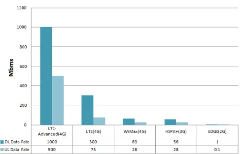
The theoretical peak for the downlink (DL) data rate with LTE-Advanced is 1 Gbps and for uplink (UL) the peak data rate is 500 Mbps [4]. This is much higher than any mobile network has been capable of before. The theoretical peak data rates are shown in Figure 1.

Figure 1. The theoretical peak data rates of different mobile networks.

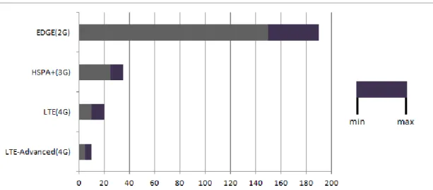
LTE and later LTE-Advanced have also been able to reduce the network latency significantly, which is seen in Figure 2. It is obvious that the mobile networks have come a long way regarding data traffic, but the customer need for faster mobile networks is growing constantly.

(10)

Figure 2. The theoretical minimum and maximum latencies of different mobile network technologies. (X-axis is time in milliseconds)

In 2013 the amount of global mobile devices grew to 7 billion [5]. It is predicted that the amount of mobile devices in use will surpass the 7.1 billion people on earth in the year 2014 [6]. Also according to Cisco, the global mobile data traffic will increase nearly 11-fold between 2013 and 2018 [5]. This creates great demand for capable mobile communication networks and the performance of those networks is of high importance.

1.2. Scope of the thesis

The Evolved Node B (eNodeB) is a LTE network element that communicates directly with user equipments (UEs). The LTE User-Plane radio interface protocols include the Layer-1 (L1) Physical Layer protocol as well as the Layer-2 (L2) protocols, i.e. Medium Access Layer (MAC), Radio Link Control (RLC) and Packet Data Convergence (PDCP) protocols.

In this thesis, we are interested in the performance of the LTE user plane protocol stack between the UE and eNodeB. These protocols and their functions are extensively described in Chapter 2.

All the data packets are processed by the PDCP, RLC and MAC before being passed to the physical layer for transmission [1]. This means that the functionalities in these protocols need to be executed efficiently and fast. The time spent in these protocols must be relatively low compared to the time it takes for the actual transmission of information. These protocols are complex and most of their implementation depends on the software. Also the 4G standard development & customer specific requirements create more pressure on software for continuous performance optimization. In this thesis the focus is on the PDCP, RLC and MAC layers of one eNodeB product and their performance characteristics, measurement and optimization.

(11)

1.3. Thesis structure

In Chapter 2 the Evolved Node B architecture and the role of the hardware and software in it is introduced. Chapter 3 goes into detail about different performance optimization methods. In Chapter 4 the performance evaluation framework and tools are described. Chapter 5 shows the results of the optimization work and goes into detail about a couple of successful optimization examples. Chapter 6 reflects upon the results of Chapter 5 and discusses optimization methods left unused in the thesis. Chapter 7 summarizes the thesis.

(12)

2. LTE ARCHITECTURE

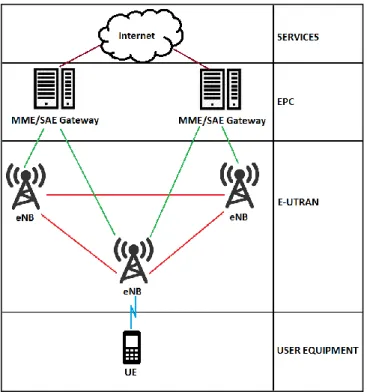
LTE Architecture can be split into four main high level domains: User Equipment (UE), Evolved Universal Terrestrial Radio Access Network (E-UTRAN), Evolved Packet Core (EPC) and the Services domain [1]. Figure 3 provides a high-level view of LTE architecture.

Figure 3. LTE Architecture overview.

The Services domain includes Operator Services and the Internet. The EPC is the core network of the LTE system. It connects the rest of the network to the Services domain. The EPC is an evolution of the packet-switched architecture used in 3G [7]. The E-UTRAN handles the communication between the UEs and the EPC and has one component, the eNodeB or eNB, which is another name for the base station [8]. The User Equipment domain contains all devices with the ability to connect to the LTE network. For example smart phones and tablet computers can be considered as user equipment.

2.1. LTE Advantages

The key difference between LTE and HSPA (3G) architecture is that there is no Radio Network Controller (RNC) in the LTE architecture. The RNC is responsible for controlling the Node Bs that are connected to it in 3G networks. In LTE the functionality of the RNC is included in the eNBs, which means that the LTE architecture has one node less than the HSPA architecture. This makes LTE architecture flat with only 2 nodes and naturally results in much faster communication between UEs and the network, which means lower latency and higher throughput.

(13)

The air interface in LTE is also different from previous generations as seen in Table 1. The multiple access schemes used in LTE are orthogonal frequency-division multiple access (OFDMA) and single-carrier frequency-division multiple access (SC-FDMA). OFDMA is used in downlink and SC-FDMA is used in uplink. OFDMA significantly increases spectral efficiency in LTE compared to HSPA and thus uses the bandwidth more efficiently and has more processing power. The reason why SC-FDMA is used in uplink is the high power consumption of OFDMA, which makes it unpractical to be used in the UEs.

The GSM architecture relies on circuit-switching (CS). This means that circuits are established between the calling and called parties throughout the telecommunication network. In GPRS and UMTS (3G) the architecture supports both packet-switching (PS) and CS. With PS technology data is transported in packets without the establishment of dedicated circuits.

The LTE architecture’s interfaces are Internet Protocol (IP) based. IP is used for control and user plane as the network layer in the protocol stack of all interfaces. The EPC is an evolution of the PS architecture used in GPRS/UMTS and CS is no longer used. This offers more flexibility and efficiency. [7]

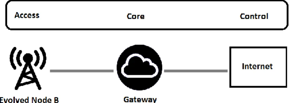
Figure 4 shows a simplified view of the LTE network. The figure highlights the importance of eNB in the LTE network. The whole LTE network depends on the capabilities of the eNB. Both the quality of software and hardware in eNB are of great importance. The faster the eNB operates, the lower the latency and the higher the throughput the user has. This chapter concentrates on the eNB and discusses its structures and complexities.

Figure 4. LTE: Flat, IP-based network.

2.2. The Evolved Node B

The eNodeB controls all radio related functions in the fixed part of the LTE system. Typically eNodeBs are distributed throughout the networks coverage area, each residing near the actual radio antennas. In short the eNodeB functions as a layer 2 bridge between the UE and the EPC. It is the termination point of all the radio protocols towards the UE, and it takes care of relaying data between the radio connection and the corresponding IP based connectivity towards the EPC. [1]

LTE, with its IP based and flat architecture, places much pressure on the eNodeB. At the functional level, the eNodeB needs to follow the 3GPP standard and be compliant with it. At the performance level, the eNodeB needs to support thousands of UEs, each with varying data rates. The high number of UEs per eNodeB, the high

(14)

data throughput and the low latency require the software and hardware of eNodeB to be optimal and well performing.

The eNodeB also has an important role in Mobility Management (MM), which means that the eNodeBs themselves are a part of the decision when to move a user under a different eNodeB. This transition usually happens when the user moves too far away from the eNodeB it is currently under. This chain of events is called a handover and is needed because a user can only be under one eNodeB at a time. [1]

The eNodeB is responsible for many Control-Plane functions, such as Mobility Management. The Control-Plane carries the control information of the network and the User-Plane carries the network’s user’s traffic.

The low latency of User-Plane is relevant nowadays for many applications such as real time gaming. Latency is measured by the time it takes for a small IP packet to travel from the UE to the internet server, and back. This is called round trip time measurement and is illustrated in Figure 5. Holma & Toskala assume that the eNodeB processing delay is 4ms and the whole round trip time of LTE network approximately 20ms. [1]

The 4ms delay target creates a high restriction for eNodeB’s performance but also leaves room for improvement. If the eNodeB’s functionalities could be performed faster, the round trip time for the whole LTE network would be less and the UE would experience less delay.

Figure 5. LTE round trip time measurement.

2.3. LTE L2 Radio Protocols

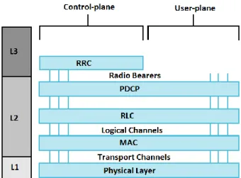
The role of the LTE radio interface protocols is to set up, reconfigure and release the Radio Bearer that provides the means for transferring the Evolved Packet System (EPS) bearer [1]. The LTE radio protocol stack is shown in Figure 6.

(15)

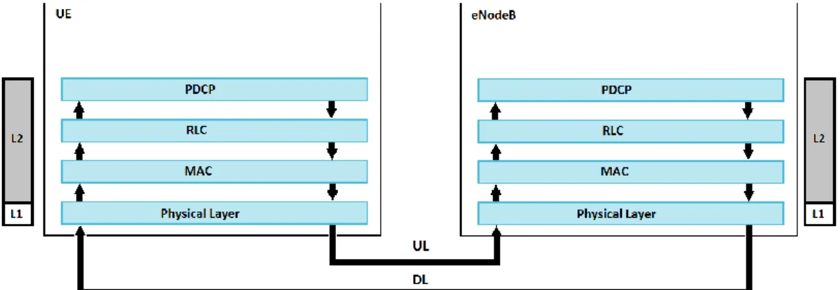
There are two types of Radio Bearers in LTE: Signaling Radio Bearer (SRB) and Data Radio Bearer (DRB). SRBs carry signaling messages and DRBs carry the user data. The term bearer can be defined in the communication system as a pipe line connecting two or more points. Therefore the EPS Bearer can be defined as a pipe line through which data traffic flows within an Evolved Packet Switched System that is the LTE network. The LTE User-Plane radio protocols between the eNodeB and the UE can be seen in Figure 7. [1]

Figure 7. LTE User-Plane radio protocols and data flow between the eNodeB and the UE.

As can be seen from Figures 6 and 7, the LTE Layer 2 (L2) consists of three sub layers:

- Packet Data Convergence Control (PDCP) - Radio Link Control (RLC)

- Medium Access Layer (MAC)

Figure 7 also shows the most important task of the LTE L2 sub layers, which is to transport data. Each sub layer naturally has additional tasks to perform in addition to transporting data but the figure illustrates the importance of performing these tasks quickly so that the data flow is as fast as possible. The faster the layers operate the faster the users can receive their data. Each layers’ task in the eNodeB side is further explained in the following subsections.

2.3.1. PDCP

The PDCP layer has three main functionalities, which are header compression/decompression of IP packets, ciphering and deciphering and integrity protection and verification.

Header compression/decompression is based on the Robust Header Compression (ROHC) protocol. Efficient compression is important especially for small IP packets because if a large IP header is created, it will be a significant source of overhead for small data rates.

Ciphering and deciphering is done for both the User-Plane and the Control-Plane. Previously in 3G networks this was done in the MAC and RLC layers.

(16)

Integrity protection and verification is done for Control-Plane data and the purpose is to confirm that the control information is coming from the correct source. [1]

The PDCP layer’s ROHC protocol is measured to be the major time critical algorithm, consuming approximately half of the entire L2 DL execution time based on measurements by D. Szczesny et al [9]. The measurements show that the computational power of the L2 DL is distributed as follows: PDCP 71 %, RLC 23 % and MAC 6 %.

2.3.2. RLC

The RLC layer transfers the protocol data units (PDUs) received from higher layers such as the PDCP to MAC layer and vice versa. The RLC also takes care of concatenation, segmentation, in-sequence delivery and error correction with automatic repeat request (ARQ). These actions are taken depending on the mode used.

There are 3 different modes in which the RLC can operate. They are Transparent Mode (TM), Unacknowledged Mode (UM) and Acknowledged Mode (AM).

Transparent Mode only relays the PDUs without adding any headers to them. This means that PDUs are not tracked. This mode is suited for services that don’t require retransmissions and are not sensitive to delivery order.

Unacknowledged Mode includes in-sequence delivery of data, which comes in handy with data that has been received out of order due to Hybrid ARQ (HARQ) operation. On the transmitting side UM mode the data is segmented/concatenated to RLC Service Data Units (SDUs) with a UM data (UMD) header. The header includes the sequence number needed for in-sequence delivery. The formed data unit is called RLC PDU and is passed on to MAC layer.

Acknowledged Mode offers, in addition to the functionalities in UM mode, PDU retransmission if they are lost in lower layers. Information on the last correctly received packet is also stored and the header has the same sequence number as in UM mode. [1]

2.3.3. MAC

The MAC layer maps the logical channels used between the MAC and RLC layer to transport channels used between the MAC and the physical layer. On the downlink side the MAC layer does the multiplexing of RLC PDUs into Transport Blocks (TB) and delivers them to the physical layer on transport channels. The MAC layer operation on the uplink side is naturally the opposite of the downlink side operation. The MAC layer also takes care of error correction through HARQ, transport format selection and priority handling between logical channels. [1]

2.3.4. Cross-layer optimization

Performance wise it is not always beneficial to split layer functionalities to be completely separate. Cross-layer optimizations remove the strict boundaries between layers to allow communication between layers. This might include one layer to access the data of another layer to exchange information for the purpose of more

(17)

efficient performance. In one study cross-layer adaptation schemes are applied to the MAC and the physical layer, which results in improved average cell throughput by 25-60% [10].

2.4. LTE layers data flow

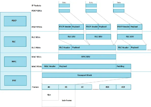
Figure 8 shows the data flow of the PDCP, RLC, MAC and the physical layer. Packets received by a layer are SDUs and the packets output of a layer are PDUs. The downlink data flow is explained in Subsection 2.4.1.

Figure 8. LTE data flow through different layers.

2.4.1. Downlink data flow

The downlink data flow starts from the IP layer, which sends packets to the PDCP layer. These packets are called PDCP SDUs. The PDCP layer then does header compression and adds a PDCP header to the PDCP SDUs. The header compression includes the removal of the IP header, which has the minimum size of 20 bytes, and adding a token, which is 1-4 bytes. Also ciphering for User and Control-Plane bearers is applied if configured. The data unit that is ciphered is the data part of the PDCP PDU. Then the PDCP layer submits the newly formed PDCP PDUs to the RLC layer.

The RLC layer receives the RLC SDUs (PDCP PDUs) and does segmentation on them. RLC segmentation might include splitting a large RLC SDU into multiple RLC PDUs or adding multiple small RLC SDUs into one RLC PDU depending on

(18)

the situation. After the segmentation is done the RLC PDUs are sent forward to the MAC layer.

The MAC layer receives the MAC SDUs (RLC PDUs) and then forms the MAC PDUs. A MAC PDU consists of the MAC header, MAC SDUs and MAC control elements. Then the MAC layer submits the MAC PDUs or Transport Blocks to the physical layer.

2.5. Focus of improvements

The improvement focus is on the software of the system rather than improving hardware or air-interface techniques. The goal is to make the LTE L2 functionalities to perform faster and to increase their capacity in users and radio bearers. In Chapter 3 many methods to boosting the performance of any embedded system by modifying its software are described.

(19)

3. PERFORMANCE OPTIMIZATIONS

Software optimization can be described as a process of modifying a software system to make some aspect of it work more efficiently or use fewer resources [11]. A program or a system can be optimized in many different ways. It can be optimized for example to:

- Execute code faster - Operate with less memory - Use memory more efficiently - Draw less power

In this chapter different software optimization methods for boosting the performance of an embedded system, like the eNodeB, are introduced. The main focus area for this thesis work is to simply decrease the load of the central processing units (CPUs) executing the software of the LTE L2 User-Plane in an eNodeB and therefore increase the capacity of the network. This translates to making the code execute faster and to use the memory more efficiently.

3.1. Compiler

Compilers translate high-level programming languages such as C and C++ into assembly code for the target processor. In the early 2000 and before, most of embedded systems were programmed using assembly, and compilers were not widely used. Embedded systems have high-efficiency requirements, thus they require well optimized software [12]. Nowadays compilers are able to offer highly optimized code and there is less need for developers to program in assembly. Each processor has its own unique machine language. In optimization context this needs to be taken into account when choosing the compiler for an embedded system [13].

3.1.1. Compiler optimization options

Compilers provide optimization opportunities by different compilation flags. With GCC compiler turning on optimization flags makes the compiler attempt to improve the performance and/or code size at the expense of compilation time and possibly the ability to debug the system. [14]

Configuring and using different compiler flags can have a huge impact in performance as is shown in the book “Techniques for optimizing applications: high performance computing”. There different optimization flags for the Sun compiler and their impact in performance are described. One example shows a part of the code, which does matrix-matrix multiplication. The performance of the code improves more than eight times when using the “–x04” optimization level in the compiler compared to compilation with no optimization. [15]

Table 2 shows the differences between a couple different GCC optimization options. The “-O3”-option is widely used with GCC compilers if optimizations are needed. From the Table differences between the 3 levels of “-O”-options can be seen. For example using the “-O1”-option the compiler inlines functions that are called once with the flag “-finline-functions-called-once“, but with the “-O3”-option the

(20)

compiler tries to inline functions more aggressively with the flag “-finline-functions”. Optimization instructions can also be given for the compiler in code with keywords and directives. The inline keyword along with others are explained in Section 3.3.

Table 2. GCC optimization options [14]

Option and description: Enables:

-O1

The compiler tries to reduce code size and execution time, without performing any optimizations that take a great deal of compilation time.

-fauto-inc-dec -fbranch-count-reg -fcombine-stack-adjustments -fcompare-elim -fcprop-registers -fdce -fdefer-pop -fdelayed-branch -fdse -fforward-propagate -fguess-branch-probability -fif-conversion2 -fif-conversion -finline-functions-called-once -fipa-pure-const -fipa-profile -fipa-reference -fmerge-constants -fmove-loop-invariants -fshrink-wrap -fsplit-wide-types -ftree-bit-ccp -ftree-ccp -fssa-phiopt -ftree-ch -ftree-copy-prop -ftree-copyrename -ftree-dce -ftree-dominator-opts -ftree-dse -ftree-forwprop -ftree-fre -ftree-phiprop -ftree-sink -ftree-slsr -ftree-sra -ftree-pta -ftree-ter -funit-at-a-time -O2

-O2 turns on all the same flags as –O1 and also some additional flags. This option optimizes even more and also increases the compilation time as well as the performance of the generated code.

-fthread-jumps -falign-functions -falign-jumps -falign-loops -falign-labels -fcaller-saves -fcrossjumping -fcse-follow-jumps -fcse-skip-blocks -fdelete-null-pointer-checks -fdevirtualize -fdevirtualize-speculatively -fexpensive-optimizations -fgcse -fgcse-lm -fhoist-adjacent-loads -finline-small-functions -findirect-inlining -fipa-cp -fipa-sra -fipa-icf -fisolate-erroneous-paths-dereference -flra-remat -foptimize-sibling-calls -foptimize-strlen -fpartial-inlining -fpeephole2 -freorder-blocks -freorder-blocks-and-partition -freorder-functions -frerun-cse-after-loop -fsched-interblock -fsched-spec -fschedule-insns -fschedule-insns2 -fstrict-aliasing -fstrict-overflow -ftree-builtin-call-dce -ftree-switch-conversion -ftree-tail-merge -ftree-pre -ftree-vrp -fipa-ra -O3

-O3 turns on all optimizations in -O2 and adds a few more in an effort to optimize even more. -finline-functions -funswitch-loops -fpredictive-commoning -fgcse-after-reload -ftree-loop-vectorize -ftree-loop-distribute-patterns -ftree-slp-vectorize -fvect-cost-model -ftree-partial-pre -fipa-cp-clone

(21)

3.2. Dynamic approach

A dynamic approach means in the scope of this thesis, making performance optimizations dynamically. One of these dynamic optimizations is compiling code on the fly, which is called dynamic compilation. Dynamic compilation is usually good for code that executes over large sets of data using the same data processing loop. In addition dynamic compilation also results in a compact binary. In this section the concept of runtime code generation is explained along with dynamic compilers and their advantages and disadvantages.

3.2.1. Runtime code generation

Runtime code generation (RTCG) means dynamically adding code to the instruction stream of an executing program. Static-code implementation translates the code into an intermediate form, which is then interpreted with a statically-compiled interpreter. With RTCG implementation code is dynamically statically-compiled, which means translating it to machine code and then executing it directly. RTCG is required for incremental compilers, dynamic linkers and debuggers. Some systems use RTCG to improve performance, such as interactive systems that demand good response time on inner loops.

Nowadays memories in embedded systems are large and fast memory is provided by caches. Fetching data fast is done by first-level caches, but if the data needed is not located in the cache, there is a large miss penalty, which has a significant effect on the performance of a system. Cache performance can be affected by implementation-dependant compiler optimizations, such as loop unrolling. RTCG lets a program dynamically adapt to these kinds of particular implementations. For example, if an array is known at runtime to be small, then the iterations can be fully unrolled. This is value-specific optimization (VSO), which means that when the program state and its inputs are known, the code can be optimized for specific values.

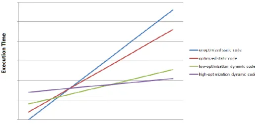
Runtime code generation is beneficial only when the generated code is run fast enough that it pays for the time spent optimizing. The payback depends on both the runtime cost of optimizing and how much faster and how many times the runtime-generated code executes. This is shown in Figure 9. [16] [17]

(22)

3.2.2. Dynamic compilers

Compilation speed is crucial to RTCG’s performance. Dynamic compilers or runtime compilers are usually faster than conventional compilers since they do not need to compile everything straight away. Some dynamic compilers are written for the particular application using statically generated templates, which contain “holes”. The dynamic compiler then later fills those holes by the values computed at runtime.

With VSO the dynamic compiler can use all information available to a static compiler with the addition of the present information visible at runtime. This leads to a high possibility of generating better code than is possible with static compilation. [16] [17]

3.2.3. Advantages

Dynamic optimizations have advantages, such as faster execution time, reduced development cost and in some cases highly optimized code compared to code produced by other methods. The faster execution time with large data sets is demonstrated in Figure 10. Dynamic optimization reduces the development costs, since it lessens the need for optimizing by hand. Also in some cases hand-written optimizations in code have fallen short to dynamic optimizations made by the compiler. [16]

Figure 10. Execution times of dynamic and static optimizations.

3.2.4. Disadvantages

Disadvantages for dynamic optimizations are: platform dependency, added complexity and the need for big data sets to be profitable. Dynamic optimizations require a lot of work and modifications to work in a specific platform. This means that if the program is needed to run on many different platforms, dynamic optimizations need to be setup to work on all of them and the solutions might be distinctly different from each other.

(23)

Added complexity means making the code hard to read. With dynamic optimizations the code needs to be modified in certain places to make use of the optimizations. When the code is harder to read, it is harder to modify and therefore the further development is increasingly difficult.

As seen in Figure 10 dynamic optimizations are great for accessing or using large data sets in processing loops. But if the code is divided into small processing loops using different data sets within them, dynamic optimizations will not provide good results.

Dynamic optimizations were not further researched in this thesis. One reason for this was that the software of LTE L2 User-Plane in eNodeB is used with multiple platforms and the platform dependency of dynamic optimizations would not fit well. Another reason was that the code in the software is packet-specific, meaning that the execution for every packet is different and therefore hard to predict and divided into many processes.

3.3. Static approach

In comparison to the dynamic approach, a static approach means, within the scope of this thesis, making optimizations by hand rather than making them dynamically in runtime. A static approach was chosen to be used in performance optimizations in this thesis. This was because static optimizations guarantee performance enhancing results, if done correctly, compared to dynamic optimizations, which could have not worked at all.

Before starting any optimizations it is vital to identify the bottlenecks of the software. A bottleneck is a component or components that limit the entire performance of a system. In some programs 99% of the time is spent doing mathematical calculations, and in some that time is spent reading and writing data files, while using them takes less than 1% of the time. Optimizing less critical parts of the code is a waste of time and will make the code more difficult to debug and maintain. This is because optimizations reduce the readability of the code and make it more complex. [18]

This section shows how to find worthwhile optimization targets. Also useful and basic optimization methods are described. The programming language used in the software of the thesis work is C++, therefore most of the examples are written in it.

3.3.1. Code profiling

Profilers help in finding the bottlenecks or hotspots of a system. Profilers are tools that can for example tell how many times a function is called, how much time it uses and where the time is spent inside that function. Profilers are not without fault and it is usually best to use more than one method in finding the bottlenecks of the software.

There are many different profiling methods. Table 3 shows four different profiling methods with explanations on how the profiling works in the method. [18]

(24)

Table 3. Different profiling methods

Profiling method What it does

Instrumentation Adds instructions to the target program to collect the required information. That information might be how many times different functions are called.

Debugging Inserts temporary debug breakpoints for example to every function or every code line.

Time-based sampling Tells the operating system to create an interrupt for example every millisecond. With the information the profiler is able to count how many times the interrupts occur in different parts of the program.

Event-based sampling Tells the CPU to generate interrupts at certain events. Events could be for example cache misses, data memory accesses and CPU cycles. This makes it possible to see which part of the program has most cache misses or CPU cycles and so on.

3.3.2. Compiler keywords

Compilers have many keywords and directives that are used for giving specific optimization instructions at specific places in code. Const and static are one of the most popular of these. They work on all C++ compilers and help the compiler to do optimizations. It is important for all software developers to understand how to use these keywords, because the more they are used the more the compiler can do additional optimizations.

Const tells that a variable is constant and will never change. This will allow the compiler to optimize the variable away in many cases. One example is shown in Code Fragment 1. There the compiler can replace all occurrences of ArraySize with the value 1000. This means that the compiler does not need to allocate any memory for ArraySize. [18]

Code Fragment 1. Const keyword example const int ArraySize = 1000;

int Array[ArraySize]; … for(int x = 0; x < ArraySize; x++) { Array[x]++; }

The meaning of a static keyword depends on the situation. In Table 4 different places where the keyword static can be applied and its impact are described.

(25)

Table 4. Static keyword descriptions

Applied to Impact Why

A non-member function Tells the compiler that the function is not accessed by any other module.

Makes inlining more efficient and enables interprocedural

optimizations. A class member function The function cannot access

any non-static data members or member functions.

It is called faster than a non-static member function.

A global variable Tells the compiler that the

variable is not accessed by any other module.

Enables interprocedural optimizations.

A local const variable Tells the compiler to initialize the variable only the first time the function is called.

Saves a lot of CPU cycles.

Interprocedural optimizations (IPO) refer to a collection of compiler optimizations or techniques used to improve performance in programs containing many frequently used functions. The difference between IPO and other compiler optimizations is that IPO analyzes the entire program, where other compiler optimizations look at smaller scope issues, such as a single function or a single block of code.

An example of applying the static keyword to a local const variable is displayed in Code Fragment 2. There function calculateVariable is called only once due to the usage of a static keyword. This means that a check must be added for the variable to see if the function has been called but execution is still faster than calling the function every time the exampleFunction is called. [18]

Code Fragment 2. Static keyword example

3.3.3. Integers, variables and operators

Integer operations are fast in most cases, regardless of the size. One thing to note is to avoid using integer sizes larger than the largest register size. For example, using 64-bit integers in 32-bit systems is inefficient.

Operations like addition, subtraction, comparison, bit operations and shift operations usually take only one clock cycle on most microprocessors. Multiplication and division are the most time consuming operations. Multiplication usually takes 4 cycles, whereas division might take up to 80 cycles, depending on the microprocessor.

It is usually more efficient to use bit shifting instead of multiplication or division, if possible. Bit shifting is possible if the values of the variables are to a power of 2. A

void exampleFunction() {

...

static const int exampleVariable = calculateVariable(1); ...

(26)

good optimizing compiler will replace multiplications with shifts, when possible, but programmers should make sure that this is done by the compiler especially in places where a lot of multiplication or division operations are executed. [18]

3.3.4. Functions

Excessive function calls may cause performance issues. The book “Optimizing software in C++” lists some of these. One of the major issues is that a lot of function calls lead the code to become fragmented and scattered in memory. This will require the CPU to jump to many different code addresses, which costs CPU cycles. There are a lot of solutions for these issues, but the most important are the following: avoiding unnecessary functions, using inline functions and avoiding nested function calls in the innermost loop.

Some coding conventions prefer that the size of a function should be only a couple lines. This is good when the functions do logically distinct tasks, but splitting functions to smaller ones should not be done only because the original function was too long. Also a critical innermost loop should always be kept inside one function, if possible. If a function has to be called inside a loop, inlining should be used.

The inline keyword is an extremely simple and powerful way for optimizing C++ programs. Inlining a function means that the place where the function is called, is replaced by the function body. The benefits from inlining are the performance gains coming from avoiding the function call, stack frame manipulation and the function return. The negative side is that inlining functions increase program size, build times and may increase the program’s execution time by reducing the caller’s locality of reference.

One example of the profits of inlining is described by Pete Isensee in “C++ Optimization Strategies and Techniques”. There a situation is described where a C++ standard library sort function ran 7 times faster than one other C standard function qsort on a test of 500 000 elements because the C++ sort function was inlined.

Inlining a function is advantageous when the function is small or called from only one place. Good compilers also inline some functions automatically but in larger programs compilers usually do not inline all functions that could be inlined. This is why developers themselves should make sure that inlining is done by the compiler in places where it should be used. An example of inlining a function is shown in Tables 5 and 6. [18] [19]

(27)

Table 5. Before inlining example Code Explanation ExampleClass.cpp --- void ExampleClass::exampleFunction_1(){ ... setExampleVariable(5); ... } void ExampleClass::exampleFunction_2(){ ... exampleVariable=FncStr::getExampleVariable(); ... } FunctionStorage.hpp --- namespace FncStr{

void setExampleVariable(int value){ m_exampleVariable = value; } int getExampleVariable(){ return m_exampleVariable; } }

Execution jumps to the addresses of setExampleVariable and getExampleVariable, when they are called.

Table 6. After inlining example

Code Explanation ExampleClass.cpp --- void ExampleClass::exampleFunction_1(){ ... setExampleVariable(5); ... } void ExampleClass::exampleFunction_2(){ ... exampleVariable=FncStr::getExampleVariable(); ... } FunctionStorage.hpp --- namespace FncStr{

inline void setExampleVariable(int value){ m_exampleVariable = value;

}

inline int getExampleVariable(){ return m_exampleVariable; }

}

Compiler converts the code in functions exampleFunction_1 and exampleFunction_2 in the following way:

ExampleClass.cpp --- void ExampleClass::exampleFunction_1(){ ... m_exampleVariable = 5; ... } void ExampleClass::exampleFunction_2(){ ... exampleVariable= m_exampleVariable; ... }

(28)

3.3.5. Branches

Modern microprocessors can achieve high performance partly due to using an instruction pipeline, where instructions are fetched and decoded in several stages before they are executed. In practice this means that the processor fetches a lot of instructions in advance before executing any of them. When the processor notices a branch, it has to decide, which of the paths it will feed to the pipeline. A branch might be a if-else, switch-case, for, while or do-while statement. If the processor feeds the instructions under the else-statement to the pipeline, when it should have fed the if-statement instructions, it can lose approximately 12-25 cycles, depending on the processor. This is called the branch misprediction penalty and the processor deciding which branch to feed to the pipeline, is called branch prediction. Branch prediction is done by algorithms that make their decision through past history of that branch and other nearby branches. [18]

Branches are usually cheap, when predicted correctly, but expensive if they are mispredicted often. Branches with a 50-50 chance of going either way will result in mispredictions 50% of the time. Naturally, this will have a negative impact on performance. Imperfect branch prediction can reduce performance by a factor of two to more than ten [20]. One simple example on how to avoid branch prediction misses is the binary lookup table, which is seen in Code Fragments 3 and 4. If the original code would cause a lot of mispredictions, it would be beneficial to use the look-up table since there the processor does not have to predict anything.

Code Fragment 3. Binary look-up table example, original code int a; bool b; … if (b) a = 4; else a = 2;

Code Fragment 4. Binary look-up table example, modified code int a; bool b;

…

Static const type lookup_table[] = {2, 4}; a = lookup_table[b];

3.3.6. Error handling

C++ offers exception handling with try, catch and throw-methods in order to recover and handle errors. They are not very efficient performance-wise and should be avoided if possible. It is more efficient to define own error-handling methods, which simply print an error message and then try to exit or shut down the program or function. [18]

Error handling code is not executed very often but needs to be checked every time. This generates considerable amount of additional instructions to functions. In small scale this is not an issue, since jumping over error handling code does not have an impact on performance, if the program only has error handling in only a few parts of

(29)

the code. But in a larger scale error handling increases the size of the binary a great deal and generates a lot of inactive code.

One solution for optimizing error handling code is to move the error handling code to its own functions and make sure that it is not inlined. This is because the amount of generated instructions of an error handling code should be minimized in performance critical parts of the code.

3.3.7. Out-of-order execution

Out-of-order execution (OoOE) is an important term to understand for software developers, especially if their program is running on a microprocessor with OoOE support. If a processor has OoOE support, it executes instructions based on the availability of the input data, rather than their original order. With the help of out-of-order execution, the processor minimizes its idle time by not having to wait for the current instruction to finish before executing the second one. Code Fragment 5 and Table 7 show the advantage of out-of-order execution in a simplified example. There out-of-order execution completes the instructions 2 CPU cycles faster than in-order execution.

Code Fragment 5. Instructions of out-of-order execution example. Incrementing a variable takes one CPU cycle and loading a variable takes 4 CPU cycles

INCR A LOAD B INCR B INCR C INCR D

Table 7. Out-of-order execution example

Cycles Out-of-order execution In-order execution

1 INCR A INCR A 2 LOAD B LOAD B 3 INCR C - 4 INCR D - 5 - - 6 INCR B INCR B 7 - INCR C 8 - INCR D

One limit for OoOE is data dependency, which is also shown in the previous example. This means that for example, if the first instruction is to load variable A from memory and the second instruction is to increment that value, it cannot execute the second instruction before the first is completed.

3.3.8. Software pipelining

Software pipelining is defined as a coding technique that overlaps operations from various loop iterations in order to exploit instruction level parallelism (ILP) [21]. Software pipelining is a type of out-of-order execution, except that the reordering of

(30)

instructions is done by the compiler instead of the processor. ILP is a measure of how many operations can be performed simultaneously. If the developers want to make use of software pipelining, they must be aware of the architecture of the processor they are using. The important thing is to know how many instructions can be executed parallel and what kind of execution pipelines exist in the processor core.

For example, a fictional processor could dispatch 3 instructions parallel and have one load, one store, one simple logic, one multiply and one division execution pipeline. This practically means that it could execute simultaneously 3 operations, if the operations were different from each other. For example, it could do store, load, simple logic operation simultaneously, but could not do store, store, load simultaneously. In practice software pipelining is re-arranging code and the goal is to be able to execute instructions simultaneously as much as possible.

One example is shown in Code Fragment 6 and Table 8. There a loop is shown where in the first cycle one instruction is executed. In the second cycle two instructions are executed parallel and finally in third cycle three instructions are executed parallel to the point when there are only three instructions left in total. This is enabled by OoOE and software pipelining. The reason why three instructions cannot be executed at once from the start is the data dependency. Incrementing a variable before loading it is not possible.

Code Fragment 6. Software pipelining example for (int i = 0; i < 100; i++)

{

x = A[i]; x++; A[i] = x; }

Table 8. Instructions and their execution order of Code Fragment 6

CPU cycles i = 0 i = 1 i = 2 i = 3

1 load A[0] - - -

2 incr A[0] load A[1] - -

3 store A[0] incr A[1] load A[2] -

4 store A[1] incr A[2] load A[3]

5 store A[2] incr A[3]

6 store A[3]

3.4. Memory optimizations

Memory plays an important role in the performance of embedded systems, such as the eNodeB, since the main task of the software of LTE L2 User-Plane is to transport data from the IP layers to the physical layer and vice versa. Therefore it is essential

(31)

that the software accesses its memory as fast as possible, since usually slow memory accesses are the most time consuming operations in embedded systems.

Nowadays with the new processors pushing the limits of high performance even further, the processor-memory gap widens and becomes the bottleneck in achieving high performance [22]. This section introduces CPU caches and their importance in performance optimizations. Also, different methods for optimizing the usage of CPU caches are discussed.

3.4.1. CPU caches

CPU caches try to bridge the gap between the CPU and the memory as they offer the illusion of a large and fast memory [23]. They are a much smaller memory and they try to keep the most frequently used data copied from the main memory. Usually CPUs have three independent caches as can be seen in Table 9.

Table 9. Cache types and their function

Cache type Speeds up

Instruction cache Executable instruction fetch

Data cache Data store and fetch

Translation lookaside buffer (TLB) Virtual-to-physical address translation

Data caches are usually split into a hierarchy of more cache levels. Figure 11 illustrates one of these hierarchies in a 4-core Shared Cache Chip Multiprocessor (CMP). It has on-chip core-specific L1 Instruction caches, L1 Data caches and a shared L2 Data cache between cores.

Figure 11. A 4-core CMP cache hierarchy.

3.4.2. Cache entry structure

The data copied from main memory is stored in a cache as cache lines (also known as cache rows). When a cache line is copied from memory into the cache, a cache entry is created. The usual structure of a cache entry is shown in Figure 12.

(32)

Figure 12. Cache entry structure.

Tag contains the address of the data fetched from the main memory. Data block contains the actual data. Flag bits indicate the state in which the cache line is. Data cache typically has two flag bits: a valid bit and a dirty bit. Valid bit indicates if the cache line is loaded with valid data. Usually valid bits are set to invalid in all cache lines when the hardware powers-up. This way the CPU knows when the cache lines are stale. Dirty bit, when set, indicates that the cache line has changed since it has been copied from main memory.

3.4.3. Cache entries

In read or write operations the processor first checks whether, the required data is located in the cache. If so, the processor performs the operation for the data located in the cache, if not the operation will be performed to the data located in the main memory, which is much slower. When the processor tries to handle data which is not located in cache, it is called a cache miss. When the data is found in the cache, it is called a cache hit.

In the case of a cache hit, the processor immediately reads or writes the data in the cache line. When a cache miss occurs, the cache allocates a new entry and copies the data from the main memory. The processor has to wait for the data to be ready in the cache to perform its read or write operation. CPU caches are a critical component of any high performance system and usually cache access time and cache misses are the single factor most constraining performance, since accessing main memory is much slower than accessing caches[24].

3.4.4. Cache replacement policy

Cache replacement policy determines which data stays in the cache and which is evicted. This is needed when cache misses happen and something is needed to be replaced to make room for the new entry. One of these policies is the least-recently used policy (LRU). It replaces the least recently accessed entry with the retrieved data. In one study different replacement policies are compared and their performance evaluated and it shows that there are substantial differences in performance of different replacement policies. [25]

3.4.5. CPU stalls

When a cache miss happens, the CPU will try to execute other instructions as much as possible, while fetching the cache line from memory. Usually though the CPU will run out of things to do before the fetching is complete. This is called a CPU stall and it is basically a moment where no instructions are executed and the CPU is idling. This of course should be avoided since it can cost hundreds of wasted CPU cycles. The penalty of a cache miss depends on how good the CPU is able to

(33)

hide it. The more the CPU can issue instructions during the cache miss, the better the penalty is hidden. [26]

The focus of the thesis in memory optimizations is mainly to try to avoid cache misses as much as possible. If avoiding a cache miss is not possible, then the penalty of the miss must be minimized. Techniques for avoiding cache misses and minimizing the penalty are described in the subsections to follow and in Section 3.5.

3.4.6. Code arrangement

Functions that are used near each other should be also stored near each other. The code cache benefits from this and works more efficiently. Also, it is efficient to collect functions that are used in the critical part of the code and store them together preferably in the same source file. Seldom used functions and code like error handling should be put to their own functions and be kept separate from often used functions.

Variables should be declared before they are needed inside functions and variables and objects like functions that are used close together should also be stored together. Static and global variables and dynamic memory allocation should also be avoided. [18]

3.4.7. Prefetching

Fetching a cache line that is expected to be used later is called prefetching. This is done to avoid cache misses that would happen without prefetching. Modern processors do prefetching automatically quite efficiently thanks to out-of-order execution and advanced prediction mechanisms. Prefetching is one of the several effective approaches for tolerating large memory latencies [18]. There are two main ways of prefetching: prefetching initiated by hardware and prefetching initiated by software.

Hardware prefetching is implemented by the processor. The implementation of the hardware prefetching is naturally different in different processors. Nowadays processors have multiple different hardware prefetchers, such as for example Intel Xeon® 5500 series processors, which have separate prefetchers for fetching data to L1 cache and for prefetching data to L2 caches. Hardware prefetchers can have different algorithms that decide which cache lines are fetched. One algorithm could always fetch two adjacent lines, where one could monitor data access patterns and try to predict from them the addresses needed in the future.

Software prefetching is done by the software developers manually. When doing software prefetches, the developers must have knowledge of the possible places where prefetching is needed. Different performance profilers can help in this by providing information on where, for example, CPU stalls happen. Doing software prefetching generally helps, but without performance profiling information it can harm the system’s performance.

Prefetching has to be done in the correct time. Prefetching too early will result in replacing useful data or in worst cases the prefetched data will be replaced before being used. If prefetching is done too late, it will not be able to hide the processor stall. Figure 13 illustrates the effect of a successful prefetch on execution time. [27] [28]

(34)

Figure 13. Prefetching example.

3.5. Loop optimization

The efficiency of a loop depends on the processor’s ability to predict the loop control branch. An optimal loop, which is small and has a fixed repeat count with no branches inside, can be predicted perfectly. But in practice those loops are rare. [18]

Loop optimization is the process of optimizing loops, which results in faster execution time and less overhead. It boosts cache performance and uses parallel processing to its advantage. Loop optimizations are also very important since most of the execution time is spent inside loops. [29]

Extensive research has been done on loop optimizations and there are many different methods of doing them. The following subsections go through a couple of those methods that best fit into the theme for this research. One loop optimization that has been already described in Subsection 3.3.8 is software pipelining.

3.5.1. Loop unrolling

Loop unrolling is a technique that attempts to optimize a program’s execution speed at the expense of binary size. It writes the loop or part of the loop open when used. Loop unrolling is helpful when a loop contains branches. It is able to remove those branches when done correctly and will also reduce the loop control branch significantly.

Code Fragments 7 and 8 show one example. Advantages of the loop unrolling are: loop control branch count reduced to 10 from 20 and the if-branch is removed completely. The disadvantage is that the unrolling creates more code to the binary. Overall the execution speed will increase by this change.

(35)

Code Fragment 7. Loop unrolling example, original code for (int x = 0; x < 20; x++) { if (x % 2 == 0) { exampleFunction_A(x); } else { exampleFunction_B(x); } exampleFunction_C(x); }

Code Fragment 8. Loop unrolling example, unrolled loop for(int x = 0; x < 20; x+=2){ exampleFunction_A(x); exampleFunction_B(x+1); exampleFunction_C(x); exampleFunction_C(x+1); }

Some compilers like the GCC can unroll loops in the code automatically. In GCC this is done by enabling the flag “-funroll-loops”. This option makes the code larger, but may or may not make the code run faster [14]. Loop unrolling should be done by the developer manually only if it appears beneficial, such as for example in the previous example, where the if-branch was eliminated. [18]

3.5.2. Loop fusion/fission

One obvious method for loop optimizations is the loop fusion. There two or more for-loops are combined into one, if the loops iterate over the same range and do not have data dependencies on each other. It might seem that loop fusion would always improve performance but this is not the case. In some cases two loops may perform better than one loop, which might be caused for example if the one loop contains an excessive number of computations. One example of loop fusion is illustrated in Code Fragments 9 and 10.

Code Fragment 9. Loop fusion example, original code for (int x = 0; x < 100; x++){ A[x] = A[x] + 5; } for (int x = 0; x < 100; x++){ B[x] = B[x] + 10; }

Code Fragment 10. Loop fusion example, combined loop for (int x = 0; x < 100; x++){

A[x] = A[x] + 5; B[x] = B[x] + 10; }