Hilbert-Huang Transform for ERP detection

(1)

Z´

apadoˇ

cesk´

a univerzita v Plzni

Fakulta aplikovan´

ych vˇ

ed

Hilbert-Huangova transformace

pro detekci evokovan´

ych

potenci´

al˚

u

Ing. Jindˇrich Ciniburk

disertaˇ

cn´ı pr´

ace

k z´ısk´

an´ı akademick´

eho titulu doktor

v oboru Inˇ

zen´

yrsk´

a informatika

ˇ

Skolitel: Prof. Ing. V´

aclav Matouˇsek, CSc.

Katedra informatiky a v´

ypoˇ

cetn´ı techniky

(2)

University of West Bohemia

Faculty of Applied Sciences

Hilbert-Huang Transform for

ERP detection

Ing. Jindˇrich Ciniburk

dissertation thesis

submitted in partial fulfillment of the requirements

for a degree of Doctor of Philosophy

in Computer Science and Engineering

Supervisor: Prof. Ing. V´

aclav Matouˇsek, CSc.

Department of Computer Science and Engineering

(3)

Declaration

I present a dissertation thesis to be reviewed and defended. The thesis was created at the end of doctoral study on Faculty of Applied sciences, University of West Bohemia. I hereby declare that I have created this work alone if not noted otherwise and that all used references are properly cited in a list at the end of this thesis.

In Pilsen, 29th_August,₂₀₁₁ _{. . . .} Ing. Jindˇrich Ciniburk

(4)

Abstrakt

Pˇri vyhodnocován´ı ERP experiment˚u je naprosto nezbytné pˇresnˇe urˇcit am-plitudu a latenci jednotlivých ERP komponent. Protoˇze je EEG signál kvazi-stacionárn´ı, je nezbytné pro jeho analýzu pouˇz´ıt ˇcasovˇe-frekvenˇcn´ı metody, jako je waveletová transformace, krátkodobá Fourierova transformace, nebo matching pursuit. Dalˇs´ım zástupcem metod ˇcasovˇe-frekvenˇcnˇe analýzy je Hilbert-Huangova transformace, která byla navrˇzena pˇr´ımo pro zpracován´ı nestacionárn´ıch signál˚u. V mé práci jsem navrhl nˇekolik modifikac´ı Hilbert-Huangovy transformace, které umoˇzn´ı omezit tzv. overshoot efekt, který vzniká v pr˚ubˇehu vytváˇren´ı obálek. S navrˇzenými vylepˇsen´ımi jsou pˇr´ıdavné extrémy lépe um´ıstˇeny, t´ım je zajiˇstˇena vyˇsˇs´ı rychlost rozkladu na intrinsic mode funkce a z´ıskané intrinsic mode funkce v´ıce odpov´ıdaj´ı p˚uvodn´ımu EEG signálu.

(5)

Abstract

While evaluating ERP experiments, it is essential to determine the amplitude and latency of ERP components. Time-frequency domain methods, such as the wavelet transform, short-time discrete Fourier transform, matching pursuit, are usually used for this task, because the EEG signal is quasi-stationary. The Hilbert-Huang transform was designed to process non-stationary signals. There-fore, it should be suitable for processing EEG signals as well.

I have designed several modifications of the Hilbert-Huang transform, which restrain the over/undershoot effect occuring when envelopes are being calculated. My modifications contribute to better estimation of additional extrema and im-prove the results acquired from processing the EEG signal (even when it is con-tamined with artifacts). They make the empirical mode decomposition faster and the decomposed IMFs corresponds more with the original EEG signal.

(6)

List of Figures

3.1 10-20 electrode placement system . . . 5

3.2 Muscles and EKG artifact [3] . . . 8

3.3 Example of eye movement artifacts [3]. . . 8

3.4 Skin artifact [3] . . . 9

3.5 Electrode artifact. Sudden change of the impedance. [3] . . . 10

4.1 Properties of ERP wave . . . 13

5.1 Latency variability could cause deformation of ERP wave, when the trials are averaged. . . 20

5.2 50Hz noise in the EEG signal and the same signal after processing with a notch-filter. . . 21

5.3 Created averaged ERP wave without baseline correction. . . 22

6.1 Dilatation of Mexican hat wavelet . . . 25

6.2 Translation of Mexican hat wavelet . . . 26

6.3 Input signal and its scalogram. . . 26

6.4 Haar wavelet (scaling function on the right, wavelet function on the left) . . . 27

6.5 Principle of Discrete Wavelet transform [34] . . . 28

6.6 Input signal with P3 component [25] . . . 32

6.7 Gabor atom which best approximates P3 component [25] . . . 32

6.8 Wigner-Ville transform of MP algorithm output [25] . . . 33

6.9 Input signal . . . 33

(11)

LIST OF FIGURES

6.11 ERP component model in the corresponding location . . . 34

8.1 Example of a signal and the spline overshoot effect. Undershoot effects are better visible in figures 8.2. . . 43

8.2 Detail of spline undershoot effects. . . 43

8.3 Demonstration of the mirror method from [28]. . . 45

8.4 The illustration of the slope based method from [28]. . . 47

8.5 Example of artificial signal which represents the EEG signal with artifacts. . . 47

8.6 Example of poorly estimated additional extrema point with mirror method. . . 48

8.7 Example of poorly estimated additional extrema with slope based method. . . 49

9.1 Misplaced additional extrema created by First/Last method . . . 51

9.2 Example of distorted IMF, caused by misplaced additional extrema. 52 9.3 Modified Mirror Method . . . 54

9.4 Envelopes created with additional extrema estimated by Modified mirror method . . . 55

9.5 Detected extrema with Inflection Point Method . . . 56

9.6 Extrema detected by Delta Difference Method . . . 57

9.7 Hilbert transform results of simple sinus wave using simple arctan 58 9.8 Hilbert transform results of simple sinus wave using arctan2 . . . 60

10.1 Class diagram of Core module of HHT . . . 62

10.2 Preview of the classifiers result . . . 71

10.3 Success preview of used classifiers . . . 73

11.1 Envelopes created using Inflection Point Method. . . 77

11.2 Envelopes created using Delta-difference method. . . 78

11.3 Comparison of Improved mirror method using Inflection point method (left) and Delta-difference method (right) for extrema detection. . 79

1 The visualization of HT results - single IMF. . . 99

(12)

LIST OF FIGURES

3 An example of decomposed IMFs of the EEG signal. . . 101 4 Time-Frequency map . . . 102

(13)

Acronyms

CCT Cauchy convergence test. CWT continuous wavelet transform.

DWT discrete wavelet transform.

EEG electroencephalography. EKG electrocardiography.

EMD empirical mode decomposition. ERP event-related potential.

FFT Fast-Fourier transform.

HAS Hilbert spectral analysis. HHT Hilbert-Huang transform.

HT Hilbert transform.

IMF intrinsic mode function.

MP matching pursuit.

SC stopage criteria.

SD standard deviation.

(14)

Chapter 1 Introduction

The electroencephalography (EEG) still has its place as a diagnostic tool in to-day’s world. It has several advantages over newer methods such as the com-puterized tomography (CT), magnetic resonance imaging (MRI), functional MRI (fMRI), positron emission tomography (PET). The greatest advantages are excel-lent temporal resolution (sampling frequency in kHz), low cost of examinations, and very low cost of the equipment. The other advantage is portability; today’s EEG devices are small enough to be used as holters. These advantages lead to acquiring long time records (often longer than 24 hours). But there is the greatest disadvantage: the only way to analyze is to conduct a visual analysis of the raw EEG recording. This is still the state of art of the clinical electroencephalography – there hasn’t been any significant progress in last 75 years [7]. The situation of the processing and analyzing event-related potentials (ERPs) is similar.

Event Related Potentials (ERPs) play the essential role in the Brain-Computer Interface, in the medicine and attention experiments. We cooperate with the University Hospital in Pilsen, Skoda Auto Inc., and Faculty of Transportation Science of Czech Technical University in Prague on assessment of the level of drivers’ attention. Our research group at the Department of Computer Sciences and Engineering, University of West Bohemia is responsible for technical and scientific issues, e.g. EEG/ERP laboratory operation, development of advanced software tools for EEG/ERP research, or analysis and proposal of signal process-ing methods.

(15)

1. Introduction

To detect an ERP component means to locate the wave and determine its amplitude and latency. There are suitable time-frequency domain methods to achieve this task, such as Wavelet transform and Matching pursuit. Matching pursuit and Wavelet transform are using predefined functions (wavelets, Gabor atoms) in which the EEG signal is decomposed to. Another alternative is repre-sented by Hilbert Huang transform, which decomposes the signal into Intrinsic Mode Functions (IMFs) defined by the signal itself. The Hilbert Huang transform was specially designed for processing non-stationary signals such as EEG.

The aim of my PhD thesis is to use the Hilbert Huang transform for EEG signal processing, especially for the ERP detection. Hilbert Huang transform is a relatively new method proposed by Huang in [10]. It seems to be very promising for the EEG signal processing because it could calculate instantaneous frequency and amplitude - tasks essential for the ERP detection.

During tests of the Hilbert Huang transform on the data acquired in our laboratory, I have encountered several drawbacks of the Empirical Mode Decom-position method (first part of Hilbert Huang Transform). Therefore, I had to design modifications which adapt the Hilbert Huang transform for EEG signal processing and ERP detection.

(16)

Chapter 2 Aims of the PhD Thesis

The PhD thesis is focused on the EEG signal processing with time-frequency methods, especially on using Hilbert Huang transform to accomplish this task.

Following objectives were defined for my PhD thesis:

1. To implement and test HHT for EEG signal processing and ERP detection. 2. To propose necessary modifications of HHT in EEG/ERP analysis

(estima-tion of first and last extrema point, stopping condi(estima-tions, etc.) 3. To design and implement HHT algorithm improved according to2.

4. To validate the proposed method in multiple experiments including tests on real world data (acquired in our laboratory).

(17)

Chapter 3 Introduction into EEG

3.1 Origin of the EEG Signal

EEG is an abbreviation of the Electroencephalogram and it is a result of the neu-rophysiologic measurement of an electrical activity emitted by the brain. This method is called the Electroencephalography. The EEG signal is a time varia-tion of potential difference between two electrodes placed on the patient’s scalp surface.

The EEG signal is created by weighted summation of signals produced by huge amount of single neurons, located in parts of the brain: cortex and thalamus. The intensity of the electric activity of neuron groups depends on the distance between the electrode and neurons. Neurons located in greater distance from the electrode contribute less to the resulting electric activity than neurons which are closer to the electrode. There is no way to separate contribution of the single neuron.

3.2 Measurement of the EEG Signal

Nowadays is the EEG recorded as a discrete signal and stored on optical discs, flash cards, hard disks and in databases. The capacity of storage media enables to keep recordings from every patient’s examination.

Each modern encephalographic recording system consists of [37]

(18)

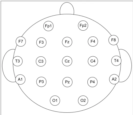
3. Introduction into EEG Fp1 Fp2 Fz F4 F8 F3 F7 T3 C3 Cz C4 T4 Pz P4 A2 P3 A1 O1 O2

Figure 3.1: 10-20 electrode placement system

• amplifiers with filters,

• an A/D converter

• and a recording device.

Electrodes are attached to the patient’s scalp and read the signal from the sur-face. To decrease the impedance between the patient’s scalp and the electrode, a conductive gel is applied. When the impedance is lower, the EEG signal is more suitable for the processing. The usual layout of electrodes for the standard EEG examination was established in 195. It is called 10-20 electrode placement system [37] (see figure 3.1. However the count of the used electrodes could be greater or lower (e.g. five or even three electrodes are sufficient for some event related potentials experiments).

(19)

3. Introduction into EEG

The EEG signal acquired from the patient’s scalp is too weak (µV) to activate the differential amplifier. It has to be pre-amplified before the amplification or processing (A/D converter). There are pre-amplifiers (usually the Common-Emitter amplifiers (see more int [36])) designed special for this task.

Before the analogue signal is converted into the discrete signal, the signal is amplified using the difference amplifier. It amplifies the difference between two electrodes. Therefore three kinds of electrodes are usually used: the ground-ing, reference electrode and active electrodes. The difference amplifiers reduce the outside interference and artifacts because they amplifies just the potential difference between two electrode distorted by the same artifact.

To store the signal on the computer, it is necessary to convert it to the discrete form. The A/D converter does this task. The signal is sampled repeatedly with the fixed time interval and each sample is converted into the digital form. a suf-ficient sampling frequency (at least two times higher than the highest measured frequency) is the requirement for a suitable A/D converter. So is the resolution -the smallest amplitude which could be sampled (it is recommended to be at least 0.5µV) [37].

3.3 Brain Rhythms

Brain waves have been categorized into five main groups according to their fre-quency range:

α The frequency of alpha waves lies within the range 8-13Hz. The amplitude is higher over the occipital areas and normally is less than 50µV. Best seen is with eyes closed and under condition of physical relaxation and relaxed awareness without any attention or concentration [23; 32].

β The frequency of beta waves lies within the range 14-26Hz (in some liter-ature no upper bound given). Higher frequencies usually called fast beta and corresponds with gamma range. Amplitude is normally up to 30µV. Beta can be found, when the patient is actively thinking or solving concrete problem [32].

(20)

γ The usual frequency range is above 30Hz, usually up to 45Hz (sometimes called fast beta). Its occurrence is very rare, it is used for diagnoses of certain brain diseases [32].

δ Delta waves are very slow 0.5-4Hz. Delta waves are associated with the deep sleep, but they could be rarely present in the waking state. They could be easily confused with artifact (caused by neck and jaw muscles). [23].

θ Waves with frequencies between 4-7.5Hz are called theta waves. Theta waves play an important role in the infancy and childhood. Normal adults have their theta activity only during drowsiness and sleep [23;32].

3.4 Interference

The acquired signal conists of signals originating in the neural activity, and sig-nals that originate from other sources than the neural activity. These recorded non-cerebral signals are termed as artifacts. Artifacts could be divided into two categories:

• physiologic

• extraphysiologic

. Physiological artifacts are generated by the patient’s body but not by the brain. Extraphysiologic artifacts come from the equipment and the environment (outside of the patient’s body)[3].

3.4.1 Physiologic Artifacts

Muscle Activity

Muscle artifacts are most common artifacts. Most often they are caused by clenching of jaw muscles (figure 3.2). Duration of the muscle artifacts is shorter than the duration of potentials generated in the brain. The frequency of muscle artifacts is in the range 50-100Hz [3].

(21)

Figure 3.2: Muscles and EKG artifact [3]

Figure 3.3: Example of eye movement artifacts [3].

Eye Movements

The eyeball acts as a dipole where the positive pole represents the cornea and the negative pole represents the retina. When the eye moves, it generates the alternate current field measurable with all electrodes near the eye (figure 3.3. The muscle artifacts, produced by muscles of the eye, influence the measured signal as well.

Glossokinetic Artifact

The tongue acts also as a dipole in the same manner as eyes. When the tip of the tongue moves, it produces broad potential field which drops from frontal to occipital areas. Frequency is variable but usually lies in the delta range [3].

(22)

Figure 3.4: Skin artifact [3]

EKG Artifact

electrocardiography (EKG) artifacts are related to the field of the heart potentials. ECG artifacts are synchronized with the ECG tracing (figure 3.2) and could be recognized through their rhythmical repetition [3].

Pulse

Pulse artifacts are caused by the pulsating vessel when the EEG electrode is placed near such vessel. Then the EEG signal contains pulse artifact with low frequency similar to the EEG activity. This artifacts correspond the ECG arti-facts (delayed 200-300ms past the ECG) [3].

Respiration Artifact

One of the respiration artifacts is slow and rhythmic. It corresponds with body movements, which affects the impedance of electrodes. The second type corre-sponds with the exhalation or inhalation and it is presented as slow or sharp waves. The second type affects the electrodes, on which the patient is lying [3].

Skin Artifact

Skin artifacts are caused by the biological artifacts which alter the impedance of the electrode. Sodium chloride and lactic acid from sweating react with the metal of electrodes and produce large and very slow waves (˜0.5Hz, figure 3.4) [3].

(23)

Figure 3.5: Electrode artifact. Sudden change of the impedance. [3]

3.4.2 Extraphysiologic Artifacts

Electrode Artifacts

When the impedance of the electrode changes suddenly, “pop” artifact (figure 3.5) appears. It is usually limited to the single electrode. The impedance of the electrode could change slowly. One of the causes is the drying-out of the conductive gel applied on the electrode [3].

Power grid 50Hz(60Hz)

This artifact is induced from external power sources like the power grid (50Hz Europe, 60Hz North America) see figure 5.2. Similar problems are caused by switched-mode power supplies. They spread interference with higher frequen-cies across the power grid. When the impedance between grounding and active electrode is significantly higher then this artifact affects the EEG signal more intensively. But it could be easily removed by using filters and lowering the grounding impedance. The common practice is to use batteries for the EEG measuring unit. The best solution would be a room shielded with Faraday cage.

3.5 Properties of the EEG Signal

If we calculate statistics of the EEG signal in different time points, we realize that these statistics vary significantly. If the statistics were nearly equal in the whole signal, the signal would be deemed as stationary. Therefore, the EEG signal is

(24)

deemed as non-stationary because its statistic differs. This is caused with the nature of the signal as it consits of different brain rhythms, artifacts, etc.

The EEG signal can be divided into the short intervals with different length but the same statistics within the interval. Such intervals are called segments and the process of acquiring them is called segmentation [32].

Nowadays the EEG is stored in its digital form only. Therefore one of the sig-nificant properties of the EEG signal is the sampling frequency. It represents the time resolution. For continuous EEG the sampling frequency up to 256Hz is suf-ficient usually. Higher sampling frequency around 1 or 2 kHz is more conventient for the ERP detection.

(25)

Chapter 4 Introduction into ERP

4.1 What is ERP?

Event-related potentials (ERPs) are EEG signals, which represent the response of the cortex to sensory, affective or cognitive events. The ERP are created as large sum of action potentials, which follow sensory or cognitive events.

The amplitude of ERPs is quite small, up to 30µV(the background EEG activity has amplitudes even 100µV). Therefore, it is necessary to use averaging technique to highlight them and suppress the background EEG [32; 39].

4.2 Properties of ERP Wave

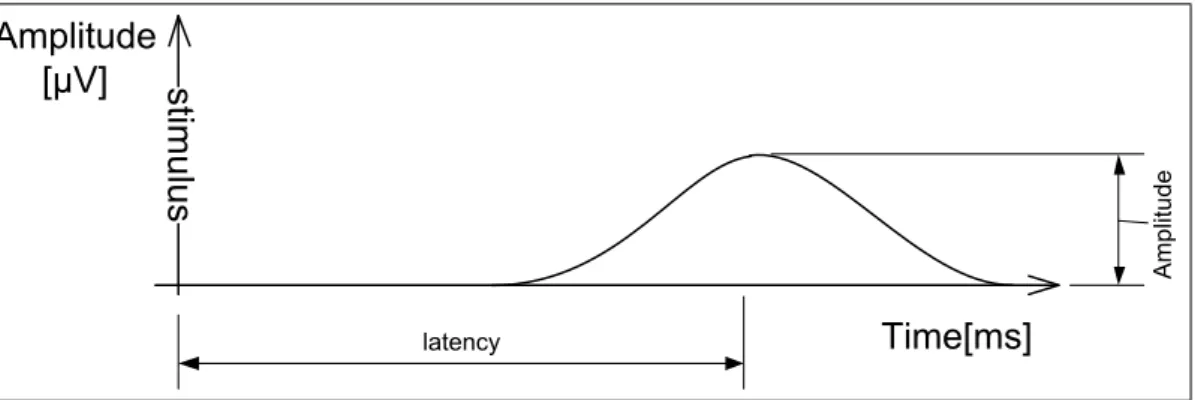
Three parameters could be used to describe ERP waves (figure 4.1):

• the amplitude,

• the latency,

• the scalp distribution.

The amplitude represents the rate of neural activity as the response to the stimulus. The latency (delay after stimulus) reveals the timing of the neural activity. The scalp distribution provides us with the information which part of

(26)

4. Introduction into ERP sti m ulu s latency A m pl itu de Time[ms] Amplitude [μV]

Figure 4.1: Properties of ERP wave

a brain was involved in the response (visual components are higher on the top of the head).

In the ideal case the amplitude will peak at the point of the ERP component. But the interference and averaging distort the ERP wave, so the maximum ampli-tude isn’t suitable for describing the ERP component. The average ampliampli-tude or the area under the curve would be a better criterion. The area under the curve isn’t so much affected by the distortion caused by averaging. When the ERP component is wider because of averaging, then the amplitude is lower, but the area under the curve remains almost same. The latency is affected in the same manner. When the averaging is performed on the ERP waves, the resulting wave-form will be “wider” (has lower frequency) and the maximum amplitude doesn’t have to be exactly in the middle of the wave (interference, artifacts). Then the better way how to establish latency, would be to divide the area below the curve (ERP component) into the two equal parts. The latency would be measured as the distance from this point (see more in [20]).

4.3 Sorts of ERPs

In this section some of the ERP components (parts of the ERP waveform) are described briefly.

ERP components are usually labeled as P1, N2, P3. The labeling refers their polarity; P for the positive and N for the negative orientation (be aware that

(27)

4. Introduction into ERP

the positive orientation is plotted downward in medical practice ). The number represents the position within the waveform. The labeling is not linked to the nature of the underlying brain activity. Therefore the the auditory component P1 and N1 are not related with visual components P1 and N1. Some of the later components such as P3 could be modality-independent, but they could contains specific sub-components.[19].

4.3.1 Visual Sensory Response

C1

C1 is the first major visual ERP component. It isn’t labeled as P or N, because its amplitude polarity can vary. Usually it is positive for stimuli in the lower visual field and negative for stimuli in the upper visual field. When it is positive it merges with P1 component usually. It starts 40-60ms after stimuli and the peak is in range 80-100ms post-stimuli. Its generation is located in primary visual cortex [19].

P1

The P1 component follows the C1 wave. P1 achieves its highest amplitude at lateral occipital electrodes. P1 onsets 60-90ms post-stimuli and its peak is located between 100-130ms. The latency of P1 varies according to the contrast of the stimulus. The P1 component is also affected by parameters of te stimulus and spatial attention (see more in [19]).

N1

After P1 wave, the N1 wave comes. The N1 component is usually divided into several sub-components. The peak of the earliest component appears after 100-150 ms at frontal electrodes. At least two posterior N1 components follow the first N1 component. They peak between 150 and 200ms after stimulus (one from parietal cortex and second form occipital cortex) [19].

(28)

P2

The N1 wave is followed by the P2 wave on frontal and central electrodes. When the stimuli contain target features and come relatively infrequently, the compo-nent is larger. In this way the P2 is similar to the P3, but the P3 can occur by far more complex target categories. The P2 wave is often overlapped with N1, N2 and P3 waves [19].

N170

The component N170 has its peak between 150 and 200ms. The N170 is later and/or larger for inverted faces used as stimuli. This effect is also observed for non-face stimuli when the subject has extensive experience of viewing these stimuli in the upright orientation. The similar effect is observed when the subject is stimulated with familiar stimuli such as words [19].

4.3.2 Auditory Sensory Response

Very Early Components

It is possible to observe a sequence of ERP peaks within the first 10 ms after auditory stimuli. These peaks are generated by various stages along the brainstem auditory pathways. Therefore these peaks are called brainstem evoked potentials (BERs) or auditory brainstem responses (ABRs). BERs are useful for testing auditory pathology, especially for infants. The BERs are followed by mid-latency components. Their latency is in range 10-50 ms. These waves arise from the medial geniculate nucleus (auditory thalamus) and the primary auditory cortex. After these waves comes the auditory P1 wave (ca. 50ms) which achieve its largest amplitudes at fronto-central electrodes [19].

N1

The auditory N1 has several sub-components like the visual N1 wave. The first fronto-central has its maximum amplitude about 75ms after stimuli and its origin is in the auditor cortex. The second wave peaks around 100 ms and the third peaks about 150ms. The latency of N1 component is affected by the attention [19].

(29)

Mismatch Negativity (MMN)

When the subject is exposed to identical stimuli and occasionally to other different stimuli called mismatching stimuli, the mismatching stimuli elicit the negative wave. This wave achieves its highest amplitude in the area of central scalp. Its latency lies between 160 and 220ms. The MMN is observed even when the subject isn’t focused on the stimuli (stimuli are not task-relevant) [19].

The N2 Family

The N2 family contains several different components. Their latency corresponds to the time range of the N2. The first one could be called the basic N2 which is elicited by repetitive non-target stimuli. If the subject is exposed to other stimuli (usually called deviants), the amplitude will be larger. If the deviants are task-relevant (differs from the MMN), then the later N2 component called N2b will be observed. This component could occur at both visual and auditory stimuli [19].

The P3 Family

In the time range of P3 wave, several different ERP components could be found. The first two of them are the P3a and P3b. The P3a and P3b are elicited by the infrequent shift in the tone or intensity (deviant stimulus), but the P3b is only present when the shift is task-relevant. The P3b component is almost always meant as the P3/P300 component (I follow this trend). The amplitude of the P3(P3b) wave is larger when the target probability is lower. The amplitude is also higher when the target-stimulus comes “unexpected”. The third factor is the attention of the subject. More is the subject focused on the task, the higher amplitude of the P3 wave is.

The P3 wave is generated after the stimulus has been processed and cate-gorized according to the task (depends on the probability of the task-relevant stimulus), therefore the P3 represents the early cognitive function of the brain (the earlier waves are just sensorical) [19].

(30)

Language related ERP components

The best known language-related component is the N400. The N400 is usually elicited as the response to violations of semantic expectancies. The N400 compo-nent could be elicited by non-linguistic stimuli [19].

4.4 Simple ERP Experiment

Let me introduce the simple ERP experiment, which I have used for acquiring the testing data. This description could clarify terminology used for the ERP experiments.

The most simple ERP experiment focused on continuous performance task. Is classic odd-ball paradigm. We have performed same experiment in our laboratory. Subject is stimulated with target stimulus letter “Q” (15%) and the non-target stimuli the letter “O” (85%). The letters are presented on the screen of the computer. The delay between two successive stimuli is 1500ms. The proband’s task was to count the occurrences of the “Q” letter (The proband doesn’t know the count before the experiment).This experiment is designed to elicit the P3b component [13;19].

The ongoing EEG signal was recorded with our BrainAmp device directly into another computer than the one presenting the stimuli. We have recorded signals from only five active electrodes P3, P4, Fz, Pz and Cz. Also the BrainAmp recorded marks for each stimuli. The stimuli marks are different for each group of stimuli (target and non-target). Therefore, each mark is described with the type of the stimulus and the time index of the sample when the stimulus presented. It is essential for ERP experiments to store these marks; without those marks it would not be possible to locate epochs in the EEG signal and to process them. We have been using sampling frequency of 1 kHz and the resolution 0.1 µV.

(31)

Chapter 5 ERP Detection Techniques

5.1 Signal to Noise Ratio

When we are processing the EEG signal to detect the ERP wave, we have to keep in mind that the amplitude of the strongest ERP wave (called P3) peaks up to 20µV, but amplitudes of common EEG rhythms are higher (α <50µV,λ <90µV

[32]). The signal-to-noise ratio (SNR) expresses this property of the signal. In our case the SNR is 20µV/90µV, it could be expressed as 0.2 as well. Such SNR is very low for simple ERP detection, but there is a technique which could increase the SNR to more suitable level. Such level of SNR could be achieved by averaging. In order to use the averaging method, there has to be enough epochs acquired during the examination process. [19].

5.2 Averaging as Basic Method for ERP

Detec-tion

It is required to increase value of SNR. The averaging technique could accomplish such task. Short epochs extracted from the continuous EEG signal are aligned with respect to the stimulus (time locking event) and mutually averaged. The i-th sample of the calculated wave is the average of N (count of averaged epochs) samples at the i-th position. This approach is based on two premises:

(32)

5. ERP Detection Techniques

• The ERP waves are assumed to be almost identical in each trial.

• The rest of the EEG signal is completely unrelated to the time-locked event (the stimuli).

When we include sufficient number of epochs in the average, the remaining noise (background EEG) will be close to the zero at every point, but the ERP wave will stay almost unchanged. The relationship between the noise R and the number of averaged trials could be expressed as (1/√N)·R (see more in [19]). There are three ways how to calculate averages:

• Stimulus-Locked (described above),

• Response-Locked

• and Time-Locked.

The stimulus-locked averaging is described above, other methods are described in the following sections.

5.2.1 Response-Locked Averages

When the latency of particular trials varies significantly (typically during experi-ments focused on reaction time), it is necessary to calculate the average by some other way than the stimulus-locked approach which could distort the wave (see more in section 5.2.3). In such cases it is better to use response-locked averages. In response-locked averaging, the epochs are aligned according to the response (ERP wave) at each single-trial.

5.2.2 Time-Locked Spectral Averaging

Another way how to calculate averages, is the Time-Locked Spectral averaging. For every epoch the time-frequency representation (time-frequency map) is calcu-lated. Discrete and Continuous wavelet transforms, Short-time Fourier transform, Matching pursuit and Hilbert-Huang transform are suitable methods for the task. The epochs are aligned to the selected time (could be stimulus) and then averages of time-frequency maps of all epochs are calculated. This approach is very useful in cases when the phase shift of the ERP waves in trials could vary.

(33)

5. ERP Detection Techniques 0 0,5 1 1,5 2 2,5 0 2 4 6 8 10 12 14 16 18 am p lit u d e time

Trial1 Trial2 Trial3 Average

0 0,5 1 1,5 2 2,5 0 2 4 6 8 10 12 14 16 18 am p lit u d e time

Trial1 Trial2 Trial3 Average

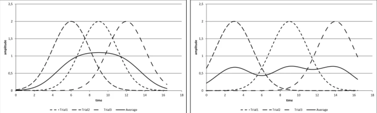
Figure 5.1: Latency variability could cause deformation of ERP wave, when the trials are averaged.

5.2.3 Latency Variability

During the averaging, we have to be very careful about the latency variability. This latency variability could lower the maximum amplitude of the ERP wave. But when the latency significantly varies, resulting averaged ERP wave could be distorted in such way that the ERP wave couldn’t be recognized at all. For the illustration, see figure 5.1.

5.3 Interference and Artifacts

There are many glitches ocurring during the averaging. We have to avoid them or minimize their impact on the resulting averaged ERP wave. Such glitches could be caused by properties of the ERP wave itself, for example by the latency variability (section 5.2.3). But distortion of the averaged ERP wave could be caused also by external influences (interference) or by signals of non-EEG origin.

5.3.1 Noise From the Power Grid

Interference coming from the power grid is always present. The noise is induced into conductors connecting the electrodes. The frequency of the noise is 50Hz (Europe) and 60Hz (North America). The interference can be easily removed with a notch-filter (see figure 5.2). The filtering has to be done before the averaging,

(34)

5. ERP Detection Techniques

Figure 5.2: 50Hz noise in the EEG signal and the same signal after processing with a notch-filter.

because there is a significant chance, that the noise doesn’t disappear during the process of averaging. Such inconvenient cases might occur, when the 50Hz sinusoid has the same phase shift in each trial. Therefore, the averaging process is not able to eleminate the interference.

5.3.2 Artifacts

Dealing with artifacts is more important task by the ERP detection than by pro-cessing of the ongoing EEG signal. Artifacts are caused usually by the muscle proband’s activity (see more in section 3.4 and [3] [16] [14]). Usually the am-plitude of artifacts is higher than 100µV; it is no exception, that artifact could have the amplitude above 200µV. Such high amplitude drives the SNR very low, making the number of trials required to be included into the average grow rapidly. Therefore, it is the common practice to exclude trials with artifacts before the av-eraging. Even better solution of this problem is to anticipate the artifacts during the experiment, instruct the proband to try not to blink (as much as possible), seat him comfortably or adapt the experiment to eliminate the artifacts as much as possible. Good data (without artifacts) are irreplaceable.

(35)

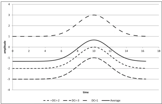
5. ERP Detection Techniques -4 -3 -2 -1 0 1 2 3 4 0 2 4 6 8 10 12 14 16 18 am p litu d e time DC=-2 DC=-3 DC=1 Average

Figure 5.3: Created averaged ERP wave without baseline correction.

5.3.3 Baseline Correction

During the running ERP experiment, proband might sweat or the conductive gel on electrodes might get dry. Both circumstances cause the change of the impedance of the electrode. As a result of both phenomena, we get the dif-ferent value of DC component for each trial. In the worst cases, changes of the impedance of the electrodes can demonstrate themselves as slow waves, that don’t belong to components of the EEG signal.

When the averaged is calculated from trials, where the DC component changes along with trials, the resulting amplitude of the averaged ERP depends on the values of DC component of each trial, not on the amplitudes of ERP waves (see figure 5.3).

This issue could be easily solved by a simple method called base-line correc-tion. Before including trials into the averaged ERP wave, the average value of first samples of the signal is calculated. The count of first samples can be derived from the latency of the first ERP component. If we are expecting that the first component comes after 100ms, we can use the first 100ms of the signal to

(36)

calcu-5. ERP Detection Techniques

late the average. Than the average is simply subtracted from the whole signal of the trial, sample by sample. This will ensure that the DC component doesn’t have the influence on the amplitude of the averaged ERP wave.

(37)

Chapter 6 Time-frequency Domain Methods

for ERP detection

For the time-frequency representation, wavelet transform (WT) and matching pursuit (MP) are often used. These two methods are suitable also for the pro-cessing of the EEG signal and ERP detection. In our team we use the WT and MP for ERP detection. Therefore, I’m going to shortly introduce the MP and WT and their application. The comparison of MP, WT and HHT will be presented in chapter 11.

The content of this chapter is taken from our common paper [53].

6.1 Wavelet Transform

Wavelet Transform (WT) is a suitable method for analyzing and processing non-stationary signals such as EEG. The WT has good ability of time and frequency localization, which is necessary for ERP detection. For the EEG signal processing it, is possible to use continuous wavelet transform (CWT) or discrete wavelet transform (DWT).

(38)

6. Time-frequency Domain Methods for ERP detection

6.1.1 Principles of Continuous Wavelet Transform

Let me demonstrate the principle of the CWT using the Mexican hat wavelet. The Mexican hat is defined as:

Ψ(t−b a ) = [1−( t−b a ) 2_]_·_e−1 2[ (t−b) a ] 2 (6.1) wherea(dilatation) corresponds with the frequency, and b(translation) describes shifting the wavelet over the signal (Figure 6.1, Figure 6.2). The translation parameter was set to 1 when we performed the CWT.

-0,6 -0,4 -0,2 0 0,2 0,4 0,6 0,8 1 1,2 0 5 10 15 20 25

a=1 a=2,5 a=4

Figure 6.1: Dilatation of Mexican hat wavelet

We have used the following algorithm of CWT for the ERP detection:

1. We have chosen the mother wavelet, set the starting and ending value of dilatation; the translation step has been set to 1.

2. We have calculated the sum of correlation for the current dilatation and repeated for every translation step in order to cover the whole signal. 3. According to the chosen step, we have changed the dilatation and continued

(39)

6. Time-frequency Domain Methods for ERP detection -0,6 -0,4 -0,2 0 0,2 0,4 0,6 0,8 1 1,2 0 5 10 15 20 25 b=4 b=8 b=17

Figure 6.2: Translation of Mexican hat wavelet

Figure 6.3: Input signal and its scalogram.

4. We stopped the run of the algorithm when the maximum dilatation value was reached.

The result of the wavelet transform is visualized in a scalogram where each coefficient represents a degree of correlation between the transformed wavelet and the signal. The scalogram is gray scaled and the highest values are white (Figure 6.3).

(40)

6. Time-frequency Domain Methods for ERP detection -1,5 -1 -0,5 0 0,5 1 1,5 -0,2 0 0,2 0,4 0,6 0,8 1 1,2 0 0,2 0,4 0,6 0,8 1 1,2 -0,2 0 0,2 0,4 0,6 0,8 1 1,2

Figure 6.4: Haar wavelet (scaling function on the right, wavelet function on the left)

6.1.2 Principles of Discrete Wavelet Transform

The continuous wavelet function, known from the CWT, is replaced by two dis-crete signals - a wavelet function and a scaling function (see Figure 6.4 for Haar wavelet example).

Given the limited spectrum band of wavelet functions, the convolution process with this function can be interpreted as a limited band-pass filter [38]. In terms of digital signal processing, wavelet transform can be considered as a bank of filters with signal decomposition into sub-frequency bands. The slowest fundamental frequency components are detected using a scale function. Wavelet function is then documented by a high pass filter and the scale function is a complementary low pass filter. Relevant coefficients are determined taking the convolution of signal and the corresponding analyzing function [34] [27]. The scale is inversely proportional to the frequency; the low frequencies correspond to large scales and to the dilated wavelet function. Using the wavelet analysis at large scales, we obtain global information from the signal (an approximate component). At small scales we obtain detailed information (a detailed component) representing rapid changes in the signal [27].

Calculation of DWT coefficients is implemented by a gradual application of wavelet function (high frequency filter) and scale function (low frequency filter) to the given signal using Mallatov decomposer scheme [1] (see Figure 6). For each level of decomposition p so-called detailed component Dp(n) of the input signal

(41)

Figure 6.5: Principle of Discrete Wavelet transform [34]

is the output of high pass filter hd(k). The approximation component A p(n) is the output of low frequency filter hd(k) Using the convolution and the subsequent subsampling the following relationships are valid [27]:

6.1.3 ERP Detection with WT

During our experiments we detected the P3 component in the EEG signal (this ERP component usually follows a stimulus with delay starting at 300 ms). When we look for the P3 component, we compute the correlation between a wavelet (which is scaled to correspond to the P3 component) and the EEG signal only in the corresponding part of the signal, where the P3 component could be situated. This approach avoids a false ERP detection in the signal parts, which couldn’t contain the P3 component. Wavelet coefficients are affected by the match of

(42)

Wavelet threshold value

Mexican hat 25

Gaussian -25

Haar 10

Daubechies6 10

Symmlet8 10

Table 6.1: Threshold values for wavelet coefficients detecting ERP component.

scaled wavelet and the signal and also by the signal amplitude. Because the degree of correlation is different for each type of wavelet we had to establish cor-responding threshold values empirically (table 6.1). To determine a threshold for ERP detection we have to preprocess EEG signal rejecting the epochs with artifacts and to correct the baseline of each epoch [34]. When the degree of corre-lation is higher than the established threshold, the ERP component is considered to be detected. Based on the threshold values given in table 6.1, Mexican hat, Gaussian wavelet, Haar and Symmlet8 were selected for the next elaboration.

The disadvantage of CWT is its computational complexity which is linearly growing according to the number of signal samples. An increase in the number of input signal samples doesn’t have so big impact if we use DWT. To detect ERP components, we use 2 kHz sampling frequency. Then the epoch, which has to be at least one second long, has 2048 samples. CWT computation on 2048 samples takes approximately 1.3 second. Therefore CWT is not suitable for BCI application [1]. We can say that the time of DWT computation on the same sample is insignificant.

6.2 Matching pursuit

The matching pursuit (MP) algorithm decomposes any signal into the sum of so-called atoms, which are selected from a dictionary. The atom that best ap-proximates the input signal, is chosen in each iteration. This atom is subtracted from the input signal and the residue enters the next iteration of the algorithm.

(43)

Averaged

Wavelet correctly false positive false negative

Epochs detected detection detection

count [%] 10 Mexican hat 32 80.0 6 2 Gaussian 33 82.0 6 1 20 Mexican hat 34 85.0 5 1 Gaussian 34 85.0 3 3 30 Mexican hat 36 90.0 3 1 Gaussian 37 92.5 2 1

Table 6.2: P3 component detection using CWT

Averaged

Wavelet correctly false positive false negative

Epochs detected detection detection

count [%] 10 Simmlet8 28 70.0 8 4 Haar 25 62.5 9 6 20 Simmlet8 33 82.5 3 4 Haar 29 72.5 6 5 30 Simmlet8 34 85.0 4 2 Haar 31 77.5 5 4

(44)

The total sum of atoms selected successively in algorithm iterations is an approxi-mation of the original signal - more iterations we do, more accurate approxiapproxi-mation we get.

The matching pursuit algorithm is most often associated with so-called Gabor atoms dictionary. Gabor atoms are defined as the Gaussian window

g(t) = e−π·t2 (6.2)

modulated using cosine function as follows

g =g(s,u,v,w)(t) = g(

t−u

s )·cos(vt+w) (6.3)

Each atom is uniquely defined by the ordered quadruple (s, u, v, w), where s denotes the scale, u is the shift,v is the frequency andw denotes the phase shift.

6.2.1 Classic ERP detection with MP

The principle of matching pursuit algorithm is to decompose the input signal into individual atoms; initially the signal trend is approximated by the atoms, secondly signal details are approximated. During recordings of the brain activity ERPs appear just like the signal trends, which are disturbed by EEG signal. After several iterations the input signal is approximated by the atoms in such a way that the signal trend is highlighted [10].

According to equation6.3each atom is uniquely defined by four values (s,u,v,w). In addition, after running of the algorithm a modulus is available for each atom. The modulus is a degree of correlation between the atom and the input signal in the iteration. The trend of the atom in time can be determined from these values. The accuracy of approximation of the original signal can be determined according to the value of the module (higher value means better approximation). ERP reflects the signal trend and the value of the modulus is high in the case of its occurrence. At the same time, the value of the shift corresponds to the loca-tion of its anticipated occurrence [25]. The idea of ERP components detection was introduced in [22].

(45)

Figure 6.6: Input signal with P3 component [25]

Figure 6.7: Gabor atom which best approximates P3 component [25]

An example of P3 components detection is shown in Figures 6.6, 6.7 and 6.8. Wigner-Villa’s transformation (see [42] and [7]) was used to display the output of the matching pursuit algorithm. This transformation shows the energy density of the signal in time frequency spectrum.

6.2.2 Principles of Modification of ERP Detection with

MP

The basic idea of the MP algorithm modification is not to base an ERP component detection on classification of feature vectors (feature vectors are parameters of

(46)

Figure 6.8: Wigner-Ville transform of MP algorithm output [25]

Figure 6.9: Input signal

Gabor atoms), but to use the MP algorithm as the method of input signal filtering and then to compute correlation between filtered (reconstructed) signal and an ERP component model.

First we approximate an input signal (figure 6.9) using several Gabor atoms and then we reconstruct the input signal from them. Loss of information caused by approximations is considered as filtering of the input signal (figure 6.10).

The nature of the MP algorithm is to suppress noise. Then the reconstructed signal corresponds to the trend of the input signal. This can be suitably used

(47)

Figure 6.10: Reconstruction of input signal from five Gabor atoms

Figure 6.11: ERP component model in the corresponding location

because ERP components are (if not discarded by artifacts) the part of the signal trend. The following phase includes the detection itself when an ERP component model (figure 6.11) is used. This model is obtained e.g. by averaging a sufficient number of epochs containing raw ERP signal or by filtering of ERP component from one epoch. The ERP component model is shifted on the restored signal in the expected range of ERP component. Correlation between the ERP component model and the reconstructed signal is computed for each shift. The maximum value of the correlation and the attaching shift value are stored. After calculating all possible correlations the stored maximum value is compared to the threshold. If the maximum value is equal to or greater than the threshold, the ERP compo-nent is detected in the corresponding location.

(48)

Averaged Matching correctly false positive false negative

Epochs pursuit detected detection detection

count [%] 10 Modified 31 77.5 7 2 Classic 26 65.0 5 9 20 Modified 34 85.0 3 3 Classic 24 60.0 9 7 30 Modified 36 90.0 2 2 Classic 31 77.5 6 3

Table 6.4: P3 component detection using MP algorithm

The results of ERP detection using modified and classic MP algorithms are available in table 6.4.

(49)

Chapter 7 Hilbert-Huang Transform

The Hilbert-Huang transform was designed to analyze nonlinear and non-stationary. The method was proposed by Huang in [11]. It consists of empirical mode de-composition (EMD) and the Hilbert spectral analysis (HAS) methods, both of these methods were introduce by Huang et al [11].

7.1 Intrinsic Mode Functions

An intrinsic mode function (IMF) is a function which has to fulfill following two conditions:

1. In the whole data set, the number of extrema and the number of zero crossings must be either equal or differ by one at most.

2. The mean value of the envelope defined by the local maxima and the local minima is zero at any point [10; 11;18].

An IMF represents simple oscillatory mode as counterpart to a simple harmonic function, but it is much more general by its definition. The conditions which IMF fulfills, are necessary for defining instantaneous frequency.

(50)

7. Hilbert-Huang Transform

7.2 Empirical Mode Decomposition

The goal of the empirical mode decomposition is to decompose the original data (signal) to the IMFs and the residue. The EMD is a data driven method and IMFs are derived directly from the signal itself [15].The most of the data are not IMFs. At any time the data may involve more than one oscillatory mode. That is why the simple Hilbert transform cannot provide the full description of the frequency. The process of acquiring the IMFs is called sifting and it’s described below [9;14; 17; 28]:

1. Initialize the residue to the original signal r0(t) = x(t) and IMF counter

i= 1

2. Extract the i-th IMF:

(a) Initialize h0(t) =ri−1(t) and initialize step counter k = 1

(b) Locate local maxima and minima inhk−1(t)

(c) Create upper envelope by connecting detected maxima with cubic spline

(d) Create lower envelope by connecting detected minima with cubic spline (e) Calculate the mean mk−1(t) by averaging the upper and lower

en-velopes

(f) Calculate hk(t) =hk−1(t)−mk−1(t)

(g) Check stopping criteria (see chapter7.2.1)

i. If stopping criteria are satisfied, then IM Fi(t) = hk(t) ii. Else k =k+ 1 and continue with 2b.

3. New residue is ri(t) = ri−1(t)−IM Fi(t) 4. Check stopping criteria of EMD

(a) Ifri(t) has at least 2 extrema then i=i+ 1 and continue with 2.

(b) Else the decomposition is finished and ri(t) is the residue after the decomposition.

(51)

7.2.1 Stopping Criteria

During the EMD we want to retrieve IMFs described in chapter 7.1. These func-tions have to fulfill two condifunc-tions. The second condition (mean of the envelopes is meant to be zero) is very difficult to fulfill. As the points 2bto2gof the EMD (from chapter 7.2) are repeated, the mean approaches to zero. But this makes amplitude variations of the individual waves more even. When we want to achieve strictly zero mean, we can assume that the amplitudes are constant and we lose very important information of the signal. So there were proposed two stopage criteria (SC). The first one is standard deviation (SD) proposed in [5; 10; 41]:

SC =SD = T X t=0 |hk−1(t)−hk(t)|2 h2 k−1(t) (7.1)

The alternative to the SD is similar to Cauchy convergence test (CCT) [9]:

SC =CCT = PT t=0|hk−1(t)−hk(t)|2 PT t=0h2k−1(t) (7.2)

The sifting process will stop when the SC is smaller than the selected thresh-old. The second stoppage criterion is based on the S-number defined as the number of consecutive sifting when the number of zero-crossings and extrema are equal or differs by one at most.

7.3 Hilbert Transform

Hilbert transform (HT) [21; 31] returns the analytic signal from real data se-quence. The analytic signal x =xr+i·xi has its real part, xr which represents the original data, and its imaginary partxi, which contains the Hilbert transform. The imaginary part is a version of the original real sequence with a 90◦ phase shift. Sines are therefore transformed to cosines and vice versa. The Hilbert transformed series has the same amplitude and frequency content as the origi-nal real data and includes phase information that depends on the phase of the original data.

(52)

The Hilbert transform is useful for calculating instantaneous attributes of time series, especially the amplitude and frequency. The instantaneous amplitude is the amplitude of the complex Hilbert transform; the instantaneous frequency expresses the rate of change of the instantaneous phase angle. In case of a pure sinusoid, the instantaneous amplitude and frequency are constant.

7.3.1 Computing Standard Discrete-Time Analytic Signal

of Same Sample Rate

The analytic signal for a sequence x has a one-sided Fourier transform (with 0 negative frequencies). To approximate the analytic signal, the Hilbert method calculates a FFT of the input sequence, replaces those FFT coefficients corre-sponding to negative frequencies with zeros, and calculates an inverse FFT of the result. In detail, Hilbert uses a four-step algorithm [31]:

1. It calculates the FFT of the input sequence, storing the result in a vector x.

2. It creates a vector h with following values:

• 1 for i = 1, (n/2)+1

• 2 for i = 2, 3, ... , (n/2)

• 0 for i = (n/2)+2, ... , n

3. It calculates the element-wise product of x and h.

4. It calculates the inverse Fast-Fourier transform (FFT) of the sequence ob-tained in step 3 and returns the first n elements of the result.

7.3.2 Representing the Result of Hilbert Transform

When we have all IMFs from EMD, we can calculate the analytic signal by using the algorithm described in section7.3.1. Calculated analytic signalZ(t) is defined as [5;10]:

(53)

Z(t) =X(t) +iY(t) = a(t)eiθ(t), (7.3)

where X(t) is the original signal, Y(t) the Hilbert transform of X(t), so the instantaneous attributes of Z(t) are defined:

a(t) =pX(t)2₊_Y₍_t₎2 _(7.4)

θ(t) = arctan(Y(t)

X(t)) (7.5)

ω(t) = dθ(t)

dt (7.6)

where a(t) is the instantaneous amplitude, θ(t) is the instantaneous phase and

ω(t) is the desired instantaneous frequency. If you want to know more about visualization see [2; 17].

7.4 Application of HHT

The Hilbert-Huang transform was designed recently, in 1998 [11]. So far it has been used in various domains where it is necessary to process linear and non-stationary data. The method has particular properties and advantages described in table 7.1. Basis functions used for decomposition are derived from data itself when the EMD is performed (other methods like Fourier, Wavelet transforms and Matching pursuit have their bases function defined a priori). The HHT derives the frequency by differentiation, therefore the HHT has no uncertainty principle limitation on time or frequency resolution [10].

The Hilbert-Huang transform (HHT) was originally designed for study of fluid mechanics [11] and in the same year used in biomedical engineering [12]. The empirical mode decomposition (EMD) has been already extended into 2D form [8]. The list of domains, where is HHT used, and interesting articles will follow:

• biomedical engineering

– Engineering analysis of biological variables: An example of blood pres-sure over 1 day [12]

(54)

Fourier Wavelet HHT

Basis a priori a priori Adaptive

Frequency Convolution: Convolution: Differential:

global, uncertainty global, uncertainty local, certainty

Presentation Energy-frequency Energy-time-

Energy-time--frequency -frequency

Nonlinear No No Yes

Nonstationary No Yes Yes

Feature Extraction No Discrete: no Yes

Continuous: yes

Table 7.1: Comparison between Fourier transform, wavelet transform and HHT [10].

– The local mean decomposition and its application to EEG perception data [33]

– a New Tool for Nonstationary and Nonlinear Signals: The Hilbert-Huang Transform in Biomedical Applications [8]

– Epileptic Seizure Detection Using Empirical Mode Decomposition [35]

• Mechanical engineering

– An improved method for restraining the end effect in empirical mode decomposition and its applications to the fault diagnosis of large ro-tating machinery [28]

• Electrical engineering

– The Application of a New Process Method for End Effects of EMD in the Insulator State Diagnosis [40]

• Economy

– Identifying the oil price–macroeconomy relationship: An empirical mode decomposition analysis of US data [24]

The HHT was successfully used for processing non-stationary data in different fields, where the high frequency-time resolution is required. Therefore, the HHT seems to be suitable for the ERP detection and EEG signal processing.

(55)

Chapter 8 Application of HHT for EEG

Processing

8.1 Creating Envelopes During EMD

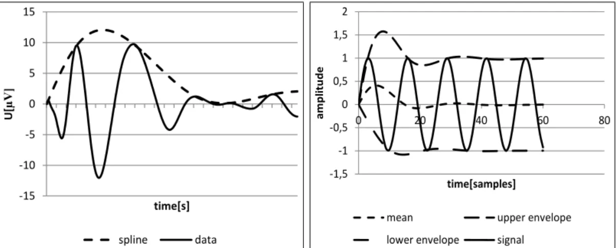
When the EMD is performed on the data series, we are trying to create upper and lower envelopes by connecting local extrema with cubic spline. Though, some difficulties surface in the process. When we want to create an envelope which covers whole signal, we have to realize that some first and last points of the signal don’t count as local extrema. The closest extremum to the beginning or the end of the signal belongs to the upper or lower envelope. Then the second closest extremum is the point from where the both envelopes are defined.

We have to add additional extremum points to extend the envelopes over the whole signal. It is the difficult part. We have to position them very carefully, because their incorrect location leads to imprecise estimate of the cubic spline (see figures8.1and8.2). This overshoots or undershoots don’t describe characteristics of the signal, but they could be propagated inward and corrupt the whole signal. The problem is described in [4; 6;29; 40; 41] in detail.

To create a complete envelope and restrain the overshoot effect, several meth-ods of additional extrema selection were proposed. They are described in follow-ing chapters.

(56)

8. Application of HHT for EEG Processing -15 -10 -5 0 5 10 15 U[ µV] time[s] spline data -1,5 -1 -0,5 0 0,5 1 1,5 2 0 20 40 60 80 am p li tu d e time[samples]

mean upper envelope

lower envelope signal

Figure 8.1: Example of a signal and the spline overshoot effect. Undershoot effects are better visible in figures 8.2.

-1 -0,5 0 0,5 1 1,5 2 U[ µ V] time[s] spline data -0,5 0 0,5 1 1,5 2 2,5 U[ µ] time[t] spline data

(57)

8. Application of HHT for EEG Processing

8.1.1 Mirror Method

Mirror method was proposed by Rilling [30] and described in [28]. The procedure is very simple. Additional extrema are mirror symmetric to the extrema that are closest to the beginning or end of the signal. The algorithm follows:

1. Locate the extremum closest to the begin of the signal (we foundM ax(1)). Then locate the extremum closest to M ax(1), this is M in(1)

2. Create new extremum on the begin of the data by creatingM in(0) respect-ing the mirror symmetry.

M inx(0) =M axx(1)−(M inx(1)−M axx(1)), (8.1)

M iny(0) =M iny(1) (8.2)

3. Repeat this process until the end of the signal is reached.

8.1.2 Slope-Base Method

The slope based method was proposed in [6] and described in [28]. This method also extends extrema, but adds one minimum and one maximum to the beginning or end of the signal. The new extrema are calculated from mathematically defined slopes created through the extrema. These slopes are derived from the distances between successive minimums and maximums and from amplitude differences. The method is shown in figure 8.4.

In the first step we have to calculate the slopes s1 and s2 for the signal x(t)

shown in the figure 8.4. The slopes are defined as:

s1 = M axy(2)−M iny(1) M axx(2)−M inx(1) (8.3) s2 = M iny(1)−M axy(1) M iny(1)−M axx(1) (8.4)

(58)

(59)

The x coordinates are defined as

∆tmax(1) =M axx(2)−M axx(1) (8.5)

∆tmin(1) =M inx(2)−M inx(1) (8.6)

M axx(0) = M axx(1)−∆tmax(1) (8.7)

M inx(0) =M inx(1)−∆tmin(1) (8.8)

Then we have to calculate the Y values of new maximum and minimum:

M iny(0) =M axy(1)−s1·(M axx(1)−M inx(0)) (8.9)

M axy(0) =M iny(0)−s2·(M inx(0)−M axx(0)) (8.10) This procedure has to be repeated in order to generate additional extrema at the end of the signal. See more in [6; 28].

8.1.3 Drawbacks of Mirror and Slope-Based methods in

EEG signal processing

When we are performing EMD on the EEG signal, we want to create envelopes covering the signal completely. The mirror method and slope based method create additional extrema to ensure this condition. The weak point of these two methods is the estimation of an additional extrema position on the time axis.

When edges of the processed signal contain time-short components of signif-icantly higher frequency (in our case artifacts), the insufficiency of methods is apparent. The problem surfaces distinctively when we use artificial signals with randomly placed artifacts (see the figure 8.5).

The example signal in the figure 8.5 starts with relatively slow frequencies but there is an artifact (with high frequency and amplitude) in the short interval after the start. Unfortunately, this artifact includes all four extrema, which we use to estimate new extrema to extend envelopes, as you can see in figures 8.6 and 8.7.

(60)

Figure 8.4: The illustration of the slope based method from [28].

-200 -150 -100 -200 -150 -100 -50 0 50 100 150 200 0 0,5 1 1,5 2 2,5 3 3,5 U[ µV ] time[s]

Figure 8.5: Example of artificial signal which represents the EEG signal with artifacts.

(61)

8. Application of HHT for EEG Processing -100 -50 0 50 100 150 200 -20 -15 -10 -5 0 5 10 15 20 25 30 35 U[µV] time[samples]

signal local extremes estimated extremes

Figure 8.6: Example of poorly estimated additional extrema point with mirror method.

When we calculate a new extremum with mirror method according to algo-rithm described in chapter 8.1.1, we get a new minimum with x-coordinate:

M inx(0) =M axx(1)−(M inx(1)−M axx(1)) = 13−(15−13) = 11 Index of a sample was used as the x-coordinate. The new minimum is at the position of the 11th _{sample. Therefore we cannot create the envelope covering} all the data. Similar problem appears when we use the slope based method to estimate x-coordinates of new extrema:

M axx(0) =M axx(1)−∆tmax(1) =M axx(1)−(M axx(2)−M axx(1))

M axx(0) = 13−(16−13) = 10

M inx(0) =M inx(1)−∆tmin(1) =M inx(1)−(M inx(2)−M inx(1))

(62)

8. Application of HHT for EEG Processing -100 -50 0 50 100 150 200 -20 -15 -10 -5 0 5 10 15 20 25 30 35 am p li tu d e time[samples]

signal local extremes estimated extremes

Figure 8.7: Example of poorly estimated additional extrema with slope based method.

We also use the index of the sample as the x-coordinate. Newly estimated extrema have its x-coordinate before the beginning of the signal. So we cannot construct the proper envelope for the sifting process (similarly described in [41].

The mirror method and slope-based method are not suitable for processing the EEG signal, because the EEG signal could contain significant changes of am-plitude and frequency (artifacts). Both methods are not able to estimate addi-tional extrema, which could determine points of complete envelopes. A significant change of amplitude and frequency is present in the processed signal; therefore, it is neccessary to design other methods for estimating additional extrema.

Hilbert-Huang Transform for ERP detection

Z´

apadoˇ

cesk´

a univerzita v Plzni

Fakulta aplikovan´

ych vˇ

ed

Hilbert-Huangova transformace

pro detekci evokovan´

ych

potenci´

al˚

u

Ing. Jindˇrich Ciniburk

disertaˇ

cn´ı pr´

ace

k z´ısk´

an´ı akademick´

eho titulu doktor

v oboru Inˇ

zen´

yrsk´

a informatika

ˇ

Skolitel: Prof. Ing. V´

aclav Matouˇsek, CSc.

Katedra informatiky a v´

ypoˇ

cetn´ı techniky

University of West Bohemia

Faculty of Applied Sciences

Hilbert-Huang Transform for

ERP detection

Ing. Jindˇrich Ciniburk

dissertation thesis

submitted in partial fulfillment of the requirements

for a degree of Doctor of Philosophy

in Computer Science and Engineering

Supervisor: Prof. Ing. V´

aclav Matouˇsek, CSc.

Department of Computer Science and Engineering

Declaration

Abstrakt

Abstract

Contents

List of Figures

Acronyms

Chapter 1

Introduction

Chapter 2

Aims of the PhD Thesis

Chapter 3

Introduction into EEG

3.1

Origin of the EEG Signal

3.2

Measurement of the EEG Signal

3.3

Brain Rhythms

3.4

Interference

3.4.1

Physiologic Artifacts

3.4.2

Extraphysiologic Artifacts

3.5

Properties of the EEG Signal

Chapter 4

Introduction into ERP

4.1

What is ERP?

4.2

Properties of ERP Wave

4.3

Sorts of ERPs

4.3.1

Visual Sensory Response

4.3.2