Assessment of Subsea BOP System
Challenges and Approaches for NewRequirements
Juntao Zhang
Reliability, Availability, Maintainability and Safety (RAMS)
Supervisor: Yiliu Liu, IPK
Co-supervisor: Laurent Bouillaut, IFSTTAR
Department of Production and Quality Engineering Submission date: June 2015
Reliability, Availability, Maintainability, and Safety
New Model for Reliability and Availability
Assessment of Subsea BOP System
Challenges and Approaches for New
Requirements
Juntao Zhang
June 2015
PROJECT / MASTER THESIS
Department of Production and Quality Engineering
Norwegian University of Science and Technology
Supervisor 1: Professor Yiliu Liu (NTNU)
Preface
This report documents my master thesis carried out during the spring of 2015. The thesis has been carried out as part of the RAMS Engineering MSc program at the Norwegian University of Science and Technology (NTNU), and is concerned with new method for reliability and avail-ability assessment and investigates different configurations of blowout preventer stack in the case study. The reader is assumed to be familiar with the terminology used in the NTNU course TPK4120 Safety and Reliability Analysis and/or the terminology used inRausand and Lundteigen (2014). The reader is also assumed to have knowledge of the basics concepts involved with subsea blowout preventer. It is further assumed that the reader has basic knowledge of the IEC61508 standard for functional safety of electric/electronic/programmable electronic safety-related systems..
Trondheim, 2015-06-16 Juntao Zhang
Acknowledgment
This master thesis could not have been carried out without the great help of a few individuals. I would especially like to thank my primary supervisor Yiliu Liu, professor at the Department of Production and Quality Engineering at NTNU, for dedicated help and support during the work. Also I would like to thank the co-supervisor Laurent Bouillaut, who works at French institute of science and technology for transport, development and networks (IFSTTAR), for his suggestions of the suitable software for carrying out the Bayesian Network analysis and answering related questions. Finally, thanks for Anne Barros for arranging the meeting with Det Norske Veritas (DNV) employees who give useful advices for my thesis work.
Summary and Conclusions
The blowout preventer system is acting the secondary safety barrier in a hydrocarbon well, where the drilling mud column is defined as the primary safety barrier. However, in pratical industry, there is a new demand for improved methods of assessing the reliability and availabil-ity of blowout preventer systems. The objective of this master thesis is to propose the relatively new method for reliability and availability assessment based on Bayesian Network, focusing on the comparsion between the various blowout preventers stack and the influence of the external information in the case study.
The thesis starting with introduction of safety critical system including the basic terminology for reliability and availability assessment. The relevant standards regarding oil and gas industry are also introduced.
The brief review about the blowout preventer is presented next. The basic structure of blowout preventer and the three main subsystems are identified and introduced. The classification of possible failure and desired functions of main components are reported. Finally, the brief re-search review about the previous reliability assessment method of subsea blowout preventer is presented, pointing out some potential weakness of the traditional methods, which indicat-ing the Bayesian Network is the one possible solution when new requirement of reliability and availability is demanded.
Then the introduction of Bayesian Network is mainly investigated for those who are not very familiar with this method. The possible allocation of Bayesian Network in reliability assess-ment and the comparsion between Bayesian Network model and the traditional method are mainly discussed. Then in the end of this chapter, there are two examples to show how the tra-ditional method used in the assessment of blowout preventer can be transferred into Bayesian Network model without losing any details, in addtion, the advanced modeling powers regarding introduction of probabilistic gates, multiple states for variables and updating information when scanerio is known are revealed in both examples.
Finally the case study about reliability and availability assessment of different blowout preven-ters is created. There are mainly three different type of blowout preventer stacks withing dif-ferent degrees of performing the desired functions under the most demanding situations. The
Bayesian Network model is able to perform such assessment effectively and one addtional in-formation is taken into account since the contribution of the wellbore pressure has significant implications on the blowout preventer’s ability to seal around or seal off the wellbore.
Finally, the conclusion and discussion are provided. The main conclusion are summarized as three key findings. First, Bayesian Network is proven to carry out the reliability and availabil-ity assessment when there is the new requirement in pratical situations, especially for updating the information when the test data is available during the operation. Second, Bayesian Network based reliability and availability assessment is possible for applying in the large scale model since it can handle probabilistic gates and multiple states of components, where the traditional method such as Fault Tree Analysis may not be able to deal with such challenges. Third, accord-ing to the analysis results of the case study, the blowout preventer equipped with the Deepwater Horizon type of stack is considered as the most reliable one in the most demanding situation, if the correct repair strategy is applied. In addition, this kind of blowout preventer is relatively very stable under the high wellbore pressure condition even though withing lower redundancy of the pipe ram subsystem, due to inclusion of casing shear ram which improves the shearing ability significantly.
Preface . . . i
Acknowledgment . . . ii
Summary and Conclusions . . . iii
1 Introduction 2 1.1 Background . . . 2
1.2 Objectives . . . 3
1.3 Delimitations . . . 4
1.4 Approach . . . 5
1.5 Structure of the Report . . . 5
2 Reliability Assessment of Safety Critical Systems 7 2.1 Basic Conceptions of Safety-Critical Systems . . . 7
2.2 Relevant Technologies and Applicable Standards . . . 8
2.3 Safety Instrumented Systems . . . 8
2.3.1 Safety-instrumented Functions. . . 9
2.3.2 Modes of Operations . . . 10
2.4 Failures and Failure Modes . . . 11
2.5 Testing Interval of SIS . . . 12
2.6 Reliability Measures . . . 12
2.7 Safety Integrity Level . . . 15
2.7.1 SIL Requirement . . . 16
2.7.2 SIL Allocation . . . 18
3 Blowout Preventer System 19
3.1 System Introduction of Blowout Preventer . . . 19
3.1.1 Main Elements of LMRP . . . 21
3.1.2 Main Elements of Blowout Preventer Stack . . . 21
3.1.3 Main Elements of Control System . . . 23
3.2 Function Identification of Blowout Preventer System . . . 24
3.3 Failure Identification of Blowout Preventer System . . . 25
3.4 Reviews of Blowout Preventer System Reliability Assessment . . . 27
4 Bayesian Network in Reliability Assessment 29 4.1 Introdution of Bayesian Network . . . 29
4.1.1 Basic Conceptions of Bayesian Network. . . 29
4.1.2 Probability Calculation of Bayesian network . . . 31
4.1.3 Building Bayesian Network Model . . . 32
4.2 Comparison between Bayesian Network and other methods . . . 34
4.3 From Fault Tree Analysis to Bayesian Network . . . 35
4.3.1 Common Cause Failure in Fault Tree and Bayesian Network. . . 37
4.3.2 Advanced Modelling Power of Bayesian Network Compared to Fault Tree . . 39
4.4 Example: Fault Tree based Bayesian Network Model . . . 40
4.4.1 Example 1: Updating information and Severity Ranking . . . 43
4.4.2 Example 2: Multiple State and Dependent Failure . . . 46
5 Case study: Reliability Assessment of BOP System in Base Case 49 5.1 Case Introduction. . . 49
5.1.1 Description of Case Study . . . 49
5.1.2 Software for Analysis . . . 53
5.1.3 Assumptions and Calculations for Input Data . . . 53
5.2 Bayesian Network Modelling . . . 56
5.2.1 Conditional Probability Tables for Model . . . 56
5.2.2 Analysis and Discussion of Results . . . 58
6 Summary 64
6.1 Summary and Conclusions . . . 64 6.2 Research Prespectives . . . 65
A Acronyms 67
B Relevant Data and Code for Case Study 70
B.1 Priors data for each subsystem in case study . . . 70 B.2 Codes for Matlab . . . 73 B.3 Analysis results of BN model . . . 75
Introduction
1.1 Background
The Macondo accident is the most severe blowout accident with the extreme consequence in oil and gas industry, recently. 11 crews were killed and the Gulf of Mexico was irretrievably polluted during this disaster. A considerable amount of literatures has investigated the main causes of the accident. Accordingly, most of them argued that the improvement of reliability assessment of safety critical system is crucial to prevent from happening again in the future. In the final report on the investigation of Macondo well blowout (Deepwater-Horizon-Study-Group,2008), they concluded that the uncontrolled blowout is caused by three categories: unrecognized risk in production casing design and construction, procedure of temporary abandonment of the well and the failure in attempting to shut-in the well such as disconnecting the drill rig from the well and activating the blowout preventer (BOP). The report also indicates that failure of the BOP as one of final barrier when dealing with well control problems is one of main causes of the accident. In the weak of the occurrence of Macondo accident, the improved reliability assessment of BOP is becoming recognized.
After reviewing standards and guidelines concerning oil and gas industries: the basic idea be-hind the safety critical system and relevant reliability assessment methods are discussed in this report. However, some weaknesses in the previous reliability study of BOP system are revealed after reviewing the BOP system, where the traditional methods is no longer adequate enough to perform the suitable analysis under the specific requirement. Since the BOP system is not only
acting as the safety barrier but also perform the operational functions, some external causes should be taken into account such as the wellbore conditions; Due to the data collection and estimation of unknown parameters of modelling, some issues such as common cause failure (CCF) have not been fully covered in the previous assessment (Hokstad and Rausand, 2008); In addition, one may expect that there is a reassessment method for updating reliability infor-mation once the testing data of BOP system is available, which means making the diagnostic analysis possible in reliability assessment of BOP system. In order to carry out the more accu-rate reliability assessment of BOP system, one appropriate probabilistic assessment model so called Bayesian Network (BN) should be introduced to face challenges upon the special features and requirement of BOP system.
This Master thesis is starting with the review of basic concepts of the reliability assessment of safety critical system. Then, the problem existing in the previous BOP reliability assessment is presented. The detailed introduction of Bayesian Network is given by descriptive examples afterwards. Firstly, two examples are created for demonstrating how the traditional method is converted into Bayesian Network and the relevant comparison between them is revealed to indicating the advantage of Bayesian Network . Then the case study is carried out by using Bayesian Network model regarding overcoming existing challenges.
1.2 Objectives
The main objective of this master thesis is to indicate the new requirement of reliability assess-ment in the existing subsea BOP system and propose the new method to fulfill those kinds of requirement. To be more specific, the objectives are:
1. Give the overall review about main concepts and approaches for reliability assessment related to safety-critical systems:
• To describe the conceptions and relevant terminology and of safety critical system, in order to help understanding the following part
• To investigate the reliability measures with different calculation methods in order to understand the difference between two major reliability measures
• To identify the safety integrity level and its requirement and allocation method 2. Present a basic understanding of BOP system, its basic structure, functions, failure modes
and relevant information
• To describe the main elements of BOP and what they are mainly used for, and present and compare the different configuration of BOP stack
• To classify essential functions and failure modes of the whole BOP system
• To identify the possible weakness or existing research gaps by reviewing the previous work
3. Introduce the suitable method for new reliability assessment in case of BOP system • To give brief introduction to the basic conceptions of Bayesian Network
• To discuss the possible solution of applying Bayesian Network in reliability assess-ment, by illustrating simple examples concerning transferring Fault Tree Analysis to Bayesian Network
4. Carry out the case study about the Bayesian Network based assessment of BOP system • To describe the current problem existing in the BOP system reliability assessment • To solve the existing problems by Bayesian Network Model
• To discuss the key findings based on the results of the analysis
1.3 Delimitations
Since viewers are supposed to have the basic knowledge in reliability assessment or relevant backgrounds, some aspects related to safety critical system and some specific calculations and formulas are only briefly investigated but not specifically described due to the limited space in this report.
In the calculation of proposed assessment method, some simplification of modeling of BOP system is made so that the loss of details is unavoidable and the operation of some components
of BOP system is not included. And some parameters are estimated by expert judgment and personal opinion of author.
1.4 Approach
• Interviews: The formulated problem is identified based on the literature review from the semester project, professional supervisions and some opinions and suggestions from the industrial companies, DNV and Rio. After discussing with experts from industry with op-eration and modelling experiences, the suitable method and the scope of the thesis is finally chosen for solutions.
• Literature research: Some contexts in this thesis are abstracted from the semester project report written by the author to avoid some unnecessary efforts, such as the summary of safety critical system, the investigation about the BOP system and the potential problems in its previous reliability assessment of BOP system.
• Case study:As suggested by supervisors, the main approach for creating Bayesian Network model in this master thesis is to use Matlab, which has the professional computational power and the specific toolbox for Bayesian Network. The instruction manual and the relevant programming can be find in the website of Bayesian Network Toolbox of Matlab (Matlab,2015).
1.5 Structure of the Report
Chapter 2 gives the overview of safety critical system conception in addition with the terminol-ogy of safety instrumented system before explanation and discussion of reliability measure and performance evaluation of related system.
Chapter 3 starts with the system familiarization of the BOP system with respect to its physical structure, and then classifies the functions and possible failure of the BOP system from the pre-vious research in reliability evaluation of the BOP system to identify the possible challenges in its traditional reliability assessment.
Chapter 4 introduces the basic ideas and rules behind Bayesian Network and its relevant cal-culations. And the detailed introduction about building Bayesian Network model is given by a simple example. Then the discussion about how Bayesian Network applying in the reliability assessment and the comparison from traditional method are given afterwards.
Chapter 5 carrys out the case study of the BOP system regarding the different configuration stack: Classical, Modern and Deepwater Horizon, which equipped with different subsystem within various redundancy. In addition, the effect of the wellbore pressure is also investigated by using the forward analysis and backward analysis.
Chapter 6 discusses the generated results from the previous chapters, especially for case study. The research respective is also proposed for future development in this area.
Reliability Assessment of Safety Critical
Systems
In this chapter, some basic terminology and conceptions about safety critical system are in-troduced briefly from subchapter 2.1 to 2.5. And subchapter 2.6 gives the introduction about reliability measures of safety critical system and how the terms are used in the calculation. In addition, subchapter 2.7 presents how to evaluate the performance of safety critical system by allocating the reliability measures.
2.1 Basic Conceptions of Safety-Critical Systems
A safety-critical system is a system whose failure may lead to harm to people, economic loss, and/or environmental damage.
—(Rausand and Lundteigen,2014) When the failure of the system would lead to the unacceptable consequence, this kind of system is called as safety-critical system. The safety-critical system is designed to perform the safety functions that can prevent equipment under control (EUC) from undesirable consequence. Note that EUC could be people in case that system is designed to protect person from harms. EUC can be protected more than one safety barrier, but all the safety barriers with respect to EUC are not necessarily safety critical system.
2.2 Relevant Technologies and Applicable Standards
Electrical,electronic,or programmable electronic (E/E/PE) technology is mostly applied in safety-critical systems (Rausand and Lundteigen,2014), often together with mechanical or other tech-nology items. The system-critical system should include at least one of E/E/PE techtech-nology. If the system excludes the E/E/PE technology, the system can use the term asSafety-related sys-tem, but it may be difficult to distinguish these two.
There are many sector-specific standards for process industry, machinery system, nuclear power plants and automotive industry. The sector-specific standards can restrict its application to the most typical and desired way of designing and operating a safety-critical system. In this master thesis, the case study is about subsea blowout preventer system, and then the standards of ap-plication of safety instrumented system in the process industry including oil and gas industry are mainly mentioned and discussed in this report. Especially the standardFunctional safety of electrical/electronic/programmable electronic safety related systems(IEC-61508,2010) and the standard Functional safety – safety instrumented systems for the process industry sector (IEC-61511, 2003) are very important standards for introducing safety related systems that involve E/E/PE technology. In addition,Norwegian oil and gas application of IEC 61508 and IEC 61511 in the Norwegian Petroleum industry (NOG-070, 2004) gives the summary of these standards and related applications in oil and gas industry.
2.3 Safety Instrumented Systems
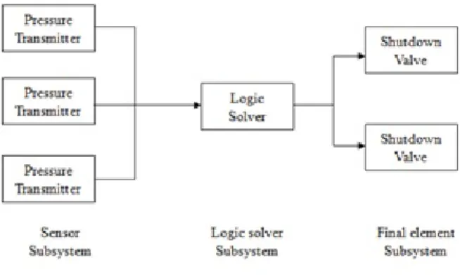
As indicated in subchapter 2.2, the system-critical system should include at least one of E/E/PE technology. This kind of system may also be referred as the term safety instrumented system (SIS) in the process industry, which is used as a protection layer between the hazards of the process and the public (Rausand and Lundteigen,2014). For the rest of report, SIS is used in line with the term in process industry instead of safety critical system. A typical SIS shown in Figure 2.1consists of at least three subsystems:sensor subsystem, logic solver subsystem and final element subsystem.
Figure 2.1: A typical SIS system
EUC and detect the undesired event and send the electrical signal to the logic solver. For example, fire and gas detectors in the process industry.
• Logic solver subsystemreceived the electrical signal from at least one sensor and determine of required actions based on the interpretation of signals. The logic solver is also consid-ered “brain” of the SIS. The programmable logic controller (PLC) is the typical logic solver automation and safety of electromechanical processes, control system, shutdown system and so forth. When the SIS hasn logic solvers, it may requirek out ofn logic solvers to agree on the following actions.
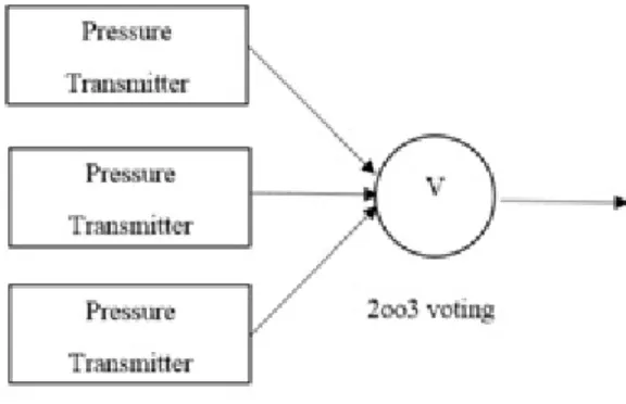
• Final element subsystemalso called asactuating devices. The function is to perform the safety function to prevent harm. The final elements could be more than one to perform the same function. A group withnidentical final elements can function when at leastk ofnchannels are functioning, then it is said to be akoon voting. As show in Figure2.2, when three valves located on the same pipeline, each can stop the pipeline therefore it is a 2oo3 voting.
2.3.1 Safety-instrumented Functions
Safety-instrumented Function (SIF) is a function that has been intentionally designed to protect the EUC against a specific demand. However, a safety function is not necessarily to be a SIF and a SIS can perform more than one SIF. Then it is imprecise to say the reliability of a SIF is the same as the reliability of the SIS or the safety loop which is performing the SIF. A SIS that implements a
Figure 2.2: 2oo3 voting system
SIF is not only designed to perform the SIF on demand, but also to keep SIF in deactivates state without the presence of demand.
2.3.2 Modes of Operations
According to the IEC 61508 (IEC-61508, 2010),demand is the condition that activates the SIF, and it is normally categorized based on how often the SIF are demanded. Normally, once per year is considered as the borderline but the rationale behind has not been clearly argued in related standards.
• Low-demand mode: is operated seldom and demanded less than once every year • High-demand mode: is operated frequently and demanded more than once every year • Continuous mode: is operated continuously. The safety function is always at demand, and
is also a special case of high demand mode.
It is important to distinguish the difference between the low-demanded mode and high/continuous mode. A SIF in EUC with low-demanded mode is usually kept passive and only activate when there is the response. A SIF that operates in high/continuous mode plays an active role in con-trol of the EUC. The importance of classification is revealed in the calculations of reliability as-sessment which would be introduced in subchapter 2.6, since the input parameter and calcu-lated formula are different based on the demand mode.
2.4 Failures and Failure Modes
Afailureis the event that terminates the ability of required function where afailure modeis to tell how the item or system fails to perform the required function (Rausand and Lundteigen, 2014). The failure rate is described as frequency of occurrence of failure in the certain time period.
The(IEC-61508,2010) also indicates two types of failures:
• The random hardware failure. It can be caused by aging, inadequate maintenance, exces-sive stress and human errors, but some analysts may not agree on that human errors and excessive stress should be classified as random hardware failure.
• The systematic faults. It is related to the deterministic cause in design phase, operational phase, documentation and other relevant factors resulting from systematic failures, which means that the appropriate modification of the design, manufacturing process and oper-ational procedures will availably eliminate such faults.
The category of hardware failures/faults based on consequence and detect ability is of vital importance in calculation of reliability of SIFs, which can be distinguished as:
• Dangerous undetected (DU) faults: This kind of failure will bring the component into fail state and can be only revealed by proof-test or occurrence of demand. The DU faults mainly contribute to SIF unavailability.
• Dangerous detected (DD) faults: This kind of failure will terminate the item to perform the required function and can be detected in the short time or immediately.
• Safe undetected (SU) failure: The failure will not cause the item to perform safety func-tions.
• Safe detected (SD) failure: The failure is not dangerous and can be detected by automatic self-testing.
2.5 Testing Interval of SIS
Test is one of the important ways to detect the potential failure, which has the significant in-fluence on the system reliability. There are two parametersintervalandcoveragecan be use to describe two types of test:
• Proof test: It is used to reveal DU failures before a demand occurs. The time region be-tween initiations of proof tests is called proof test interval. The proof test coverage is expressed as the percentage of DU failures that are detected during a proof test, which means that the higher value of coverage, then the better proof test. In general, the proof test is important to prevent DU failures in low demand system. However, it is not so evi-dent in high demand system since the demand rate is so high so that there is not enough time for high demand system to response for restoration. Then contribution of DD failure to PFH is considered as negligible.
• Diagnostic test: It is used to automatically detect the specific failure to avoid fully shut-down, usually in shorter time interval than proof test. The Diagnostic test coverage can be expressed as the ratio between the dangerous failures detected during diagnostic tests and the all dangerous failures.
2.6 Reliability Measures
Probability of failure on demand (PFD) is most widely used reliability measure in low-demand system. It can be expressed as the probability that SIF operated in low-demand mode cannot be performed at timetwhen there is a dangerous failure.
PFD(t)=Pr(The SIF cannot be performed at timet) (2.1) In the practical cases, the average value of PFD is used rather than a function of time. As as-sumptions in (Rausand and Lundteigen,2014) , a SIF is proof-tested after regular intervals of length t and the system is considered to be as good as new after proof test. Then long term aver-age probability of failure on demand can be expressed as follows, where the two key parameters
are 1) estimated failure rates from large data collection and 2) the typical test interval. PFDav g = 1 τ Z 0 τ PFD(t)d t. (2.2)
PFDavg can be interpreted in two ways according to formula:
• It can be the probability that SIF cannot be performed in response to the demand or • It is able to be expressed as mean proportion of downtime that item cannot perform
re-quired function.
For the typical SIS, the simplified equation could be easily used in calculations of PFDavg, the PFD of SIS can be the sum of the PFDs of three individual elements. This simplified equation is originally driven from Markov models, unlike Markov model, however, the time dependent fail-ures or sequence dependent failfail-ures are not involved in the simplified equation, which means that the simplified equation cannot be used for analysis of programmable logic solvers.
PFDSI S= X PFDI E+ X PFDLS+ X PFDF E (2.3)
Frequency of dangerous failure per hour (PFH) is defined as the time-dependent frequency given as number of dangerous failures per hour for SIF operated in high or continuous demand. High-demand means that the SIS is seldom proof-tested since the higher demand rate results in no time for response. The time interval (0,τ) can be the proof test interval if the SIS is proof-tested or be chosen as estimated lifetime of the SIS if the SIS is not proof-proof-tested. The average PFH in time interval (t1,t2) is
PFD(t1,t2)=
E(ND(t2))−E(ND(t1))
t2−t1
(2.4) WhereND(ti) denotes the mean number of dangerous failure in interval (t1,t2).
In the part 6 of (IEC-61508,2010), the approximation formula is calculated for a group of chan-nels or single channel and assumed the chanchan-nels are independent and any parallel structure of channels constitutes identical components. The IEC formula is calculated as follows,where two parameters are used : 1) group failure frequencyλD,G; and 2) group-equivalent mean downtime tG,E and the approximation is adequate whenλD,G tG,E is small. :
PFDav g=λD,GtG,E (2.5) In addition, there are two other parameters to derive the formulas: 1) Channel dangerous fail-ure rateλD and 2) Channel equivalent mean downtimetC,E whereith failuretG,Ei for multiple channel failures inkoonvoted group does not result in group failure.
tC,E=λDU λD (τ 2+M RT)+ λDD λD M T T R (2.6) tG,Ei =λDU λD ( τ n−k+2+M RT)+ λDD λD M T T R (2.7)
Where M RT is the mean repair time after detected failure and M T T R is the mean time to restoration.
Consider a 1oo2 system as the example, then the first dangerous failure occurs with 2λD and means downtime of a single channel is tC,E; the dangerous group failure occurs if the sec-ond channel fails when there is one failed channel. The probability is then 1−e−λDtC,Eis ap-proximated as λDtC,E if it is less than 0.1. ThenλD,G is approximated asλ2DtC,E.Then group-equivalent mean down timetG,E is equal to λλDUD (τ3+M RT)+λλDDD M T T R. The similar reduced equations are achieved for 1oo1, 1oo2, 1oo3, 2oo3, 1oo4, 2oo4.
If the CCFs is considered to contribute in IEC formulas, then the standard beta factor model is suggested to use. For 1oo2 system, theP F Dav g includes CCF can be expressed as:
PFDav g=2[(1−βD)λDD+(1−βD)λDU]2tC,EtG,E+βDλDDM T T R+βλDU(τ
2+M RT) (2.8) Whereβis the factor of common cause failure andβD indicates the fraction of detected danger-ous failures in the common cause failure factor and is usually assumed to be 0.5.
The part 6 of (IEC-61508,2010) also provides the similar approximation formulas for PFH. Then P F HG,i for akoon voted group is determined as follows, where for a 1oo1 system the PFH is equal to the frequency of DU:
PFHkoonG,i =n n−1 n−k (λ (i) D) n−k+1(λ(i) C E) n−k (2.10)
For a 1oo2 system the formula of PFH is shown as:
PFH1oo2=2[(1−βD)λDD+(1−βD)λDU]2tC,E+βDλDD+βλDU (2.11) For most of the SIS low demand mode has been assumed, and a considerable amount of liter-ature has been focused on this kind of system. In recent years, however, the research emphasis has been shifted in the discussion of high demand mode. The main differences between PFD and PFH can be driven from three aspects:
• PFD is the probability that fails to function when demand, where PFH is the frequency given as the number of dangerous failures per hour
• PFD is applied in calculation of the low demand mode where has enough time for proof-test. PFH is applied in calculation of the high demand mode or continuous mode where there is no time for response of proof test due to the higher demand rate.
• DD failure contribute less significantly to the calculation of PFH, since the demand rate is so high that there is no enough time to repair or restore the system.
When the demand rate close to once per year, the choice of these two reliability measures may lead to the different conclusion. However, conclusion has not been drawn in the Rausand’s book (Rausand and Lundteigen,2014) yet. For the further treatment of this issue, see (Jin et al.,2011) and (Liu and Rausand,2011) . In addition,Hauge(2013) provides the further discussion about choice between PFD and PFH.
2.7 Safety Integrity Level
Safety integrityis defined as the performance measure for a SIF in theIEC-61508(2010) . The Safety integrity level (SIL), measures for safety performance of the system in order to reduce the risk and increase the safety for system. SIL is divided into four, SIL1, SIL 2, SIL 3 and SIL 4, with SIL 4 being the most reliable and SIL 1 being the least.
The (IEC-61508,2010) distinguishes between hardware safety integrity, software safety integrity and systematic safety integrity. In Rausand’s book (Rausand and Lundteigen,2014), hardware safety integrity is mainly introduced and is covered partly in random hardware safety integrity. If a SIF is said to meet the SIL requirement, then each of these three integrities must be fulfilled. There is a close relationship between reliability measures and safety integrity. Safety integrity is particular application rather than generic statement since it is related to reliability measures with some specific conditions, such as stated period of time. Average PFD and PFH are mainly used for safety integrity, which has already been introduced in the previous sub-chapter 2.6. In Rausand’s book (Rausand and Lundteigen,2014), there are several important terminology issues should be noticed:
• A SIL is always related to a specific SIF instead of a SIS
• A SIL is to evaluate the whole safety loop (including sensors, logic solver, and final ele-ments) instead of any subsystem or components
2.7.1 SIL Requirement
To achieve a given SIL, there are three main types of requirements that must be fulfilled in (NOG-070,2004):
• Quantitative requirement, expressed as PFD or PFH. A quantitative analysis should in-clude random hardware failure, common cause failure and relevant failures. Separate function can be certified, but required failure probability should be verified for complete function so that the SIL requirement applies to a complete function instead of individ-ual component that perform the function. Since PFD is used as the demand rate per year, where PFH is defined as frequency per hour and one year is approximately 104hours, then there is 104difference in values between two different modes on the same SIL as observed in Table2.1.
• Qualitative requirement, expressed as architectural constraints besides PFD and PFH re-quirement which can be given in terms of three parameters:
Table 2.1: SIL for safety functions on different modes (modified from (NOG-070,2004), Table8.1)
Safety Intergrity Level Demand Mode of Operation (PFD) Continuous/ High Demand of Operation(PFH) 4 ≥10−5to<10−4 ≥10−9to<10−8 3 ≥10−4to<10−3 ≥10−8to<10−7 2 ≥10−3to<10−2 ≥10−7to<10−6 1 ≥10−2to<10−1 ≥10−6to<10−5
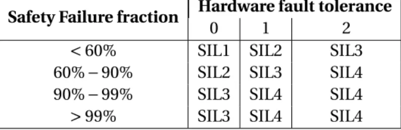
Table 2.2: Architectural constraint on type A subsystem (modified from (NOG-070,2004) , Table 8.2)
Safety Failure fraction Hardware fault tolerance
0 1 2
<60% SIL1 SIL2 SIL3
60%−90% SIL2 SIL3 SIL4
90%−99% SIL3 SIL4 SIL4
>99% SIL3 SIL4 SIL4
1. Hardware fault tolerance (HFT): in the IEC 61508 , it is defined as the digit to show the ability of a hardware subsystem to continue to perform a required function when there are faults or errors. If there is a channel that still is able to perform the required function as normal under the condition that other channels fails, then the HFT of the system is 1. For example, 2oo3 voted group is HFT=1.
2. Safe failure fraction (SFF): it is defined as in IEC 61508, the ratio of the failure rate besides DU failure to the total failure rate, where the total failure contains the safe failure SD, SU and dangerous failure DU, DD.
3. Types of subsystem: all possible failure modes can be determined for all constituent components for type A system but the behavior of type B subsystems cannot be com-pletely determined for at least one component. The relevant information is given in Table2.2and2.3.
• Avoid and control systematic faults. The systematic faults are the faults in hardware and software corresponding to design, operation and maintenance or testing. This kind of fault is not quantified in (IEC-61508, 2010) and (IEC-61511, 2003). But there are some certain measures are recommended in order to avoid and control systematic faults during
Table 2.3: Architectural constraint on type B subsystem (modified from (NOG-070,2004) , Table 8.3)
Safety Failure fraction Hardware fault tolerance
0 1 2
<60% Not allowed SIL1 SIL2
60%−90% SIL1 SIL2 SIL3
90%−99% SIL2 SIL3 SIL4
>99% SIL3 SIL4 SIL4 the design phase.
2.7.2 SIL Allocation
SIL allocation is the process in order to optimize the design to meet the SIL requirement for a SIF. The methods of SIL allocation can be categorized as:
• Qualitative methods, which determine the SIL from knowledge of risks associated to sys-tem. The typical method is Risk Graph.
• Quantitative methods, which are required to compute the reliability of SIS based on the failure rate and repair rate of components. Fault Tree Analysis (FTA), Markov approach and Petri-Nets are the well-known methods to fulfill the requirement.
• Semi-quantitative methods, which assign the value but not necessarily based on exact measurements. The most widespread method isRisk Matrix, which defines SIL accord-ing to the extent of risk and the frequency of occurrence. The other methods like Layer of Protection Analysis (LOPA) and Event Tree Analysis (ETA) are also recommended. Min-imum SIL requirement is usually used in Norwegian oil and gas industry for commonly used SIFs, which is not described in the (IEC-61508,2010) but is suggested in (NOG-070, 2004).
Blowout Preventer System
3.1 System Introduction of Blowout Preventer
The BOP system is one of the safety critical parts of the subsea drilling system since it acts as the final barrier to prevent loss of well control. In addition, the BOP system is used for a range of rou-tine operational tasks, such as casing pressure and formation strength tests (British-Petroleum, 2010).
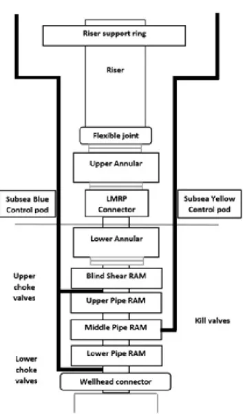
There are three important components of the BOP system: lower marine riser package(LMRP), BOP stack and control system. The BOP system includes two types of preventers: ram preventer and annular preventer. In addition, the valves and piping (choke lines and kill lines) are used to maintain pressure control in the well. A typical subsea BOP system is shown in Figure3.1. A typical subsea BOP system is equipped with five to six ram preventers and one or two annular preventers. Annular preventers are located above ram preventers since their working pressures are different from ram preventers. The typical configuration has two shear rams in order to establish a redundant system to increase the reliability. The BOP stack is attached to the well-head with a hydraulically operated, high-pressure wellwell-head connector attached the LMRP to the marine drilling riser. The detailed discussion for each main element is presented as follows (British-Petroleum,2010).
3.1.1 Main Elements of LMRP
The LMRP mainly consists of flexible joint, annular preventer, control pods, LMRP connector and choke and kill line connector:
• Flexible joint: this component is located at the top of the LMRP. It is designed to handle up to angular deflection from vertical axis of BOP (no more than 10 degree).
• Annular preventer: the function of upper annular preventer is to seal the wellbore annulus while drill pipe is running through LMRP and BOP stack. The lower annular preventer is acting as the first barrier of BOP to close around the drill pipe when there is an accident. It is installed above the ram preventers, since the working pressure of annular preventer is 10000 psi when close around the pipe and 5000 psi when close on the open hole, which is lower than the working pressure of ram preventers (Transocean,2011).
• Control pods: It provides the communication between the LMRP and BOP stack compo-nents and the surface control system. The two pods are usually called as “blue pod” and “yellow pod”, which are identical and redundant modules. There is generally a spare pod located on the rig besides the blue pod and the yellow pod. The control pods can activate all the BOP functions, which makes safety and reliability of control pods is of importance. • LMRP connector: It provides the connection between bottom of LMRP and the top of BOP stack. It allows the disconnection of the LMRP when there is the requirement of repairing control pods, and in event of an emergency or loss of rig dynamic-position station keep-ing.
• Choke and kill line connector: It connect between choke and kill lines on the LMRP and BOP stack with hydraulically operation.
3.1.2 Main Elements of Blowout Preventer Stack
BOP stack mainly consists of blind shear ram, casing shear ram, pipe ram, wellhead connector, choke and kill line valves and BOP stack hydraulic accumulators.
• Blind shear ram (BSR): it is used to cut the drill pipe and seal the wellbore and can be actuated in two modes: under 3000 psi closing pressure, or 4000 psi closing pressure. The activation of BSR is the last-option in case of emergency since it can completely seal off the wellbore, which leads to the serve damage of the equipment and rig downtime. • Casing shear ram (CSR): it is similar to the BSR when drill pipe, casing and tool joints. The
cutting ability of CSR is designed to be higher than BSR but it cannot seal the wellbore. The CSR is critical if cutting the heaviest drill pipe or casing is beyond the ability of BSR. • Pipes ram: there are three type of pipe ram based on the positions: upper, middle and
lower. They are designed to close and seal on tubular with specific range of outer diame-ter (OD). For lower pipe ram, it is usually referred as the “test ram”. Based on the design principle, there are two types: 1) standard pipe rams can seal with specific OD tolerance and 2) variable bore rams (VBR) can seal must of tubular dimension.
• Wellhead connector: this hydraulically-actuated connector can be used to connect the BOP stack to subsea wellhead housing.
• Choke and kill line valves: they are operated in fail-safe ‘close’ and can be used to isolate the choke and kill line piping connections to the BOP ram.
• BOP stack hydraulic accumulators: .The accumulator store pressurized hydraulic fluid at 5000 psi CSRs supplied from topside hydraulic power unit (HPU). It will be reduced to 4000 psi by manually-set hydraulic regulators when the accumulator bottles are used for normal closing operation of the high-pressure BSRs and high-pressure operation. The leak of accumulators will affect both pods.
There are various types of stack configurations even all BOP stacks are principally similar. For traditional BOP stack, which is still in use in many offshore locations, all the pipe rams are stan-dard and there is not any CSR installed in BOP system. The disadvantages are revealed distinctly, since the pipe ram can only seal with certain OD tolerance, which is not in favor of the redun-dancy of BOP system. Moreover, the exclusion of CSR would lead to the insufficient ability for shearing the heavy pipe.
For modern BOP stack, there is only one standard pipe ram instead of three in traditional stack for improvement in redundancy. And the modern BOP stack is equipped with the CSR for in-creasing the ability for shearing in the most demanding well control situations. This type of BOP stack is usually referred as standard stack configuration.
Deepwater Horizon (DWH) BOP stack was the one that used in Macondo well. The only differ-ence between the standard BOP stack and DWH BOP stack is the pipe rams, where pipe rams in DWH BOP stack are all VBRs and lower pipe ram is the test ram. Compared to the standard BOP stack, three VBRs increase the flexibility and redundancy to shear tubular OD to the new higher level, and the test ram reduce the prepared time before the test starts and resumed time after the test completes. However, the converting of normal pipe ram to test ram results in the loss of redundant annual sealing function since the test ram can only seal the wellbore pressure from above but not from below.
3.1.3 Main Elements of Control System
Unlike most of BOP components actuated hydraulically, the multiplexed (MUX) control sys-tem involved in performing most of the BOP desired functions is supported by both electri-cal/electronic and hydraulic components. The control systems are mounted both at topside and subsea BOP.
On the topside, the main component is the central control unit (CCU), which generally consists of two control panels: the driller’s control panel (DCP) and the toolpusher’s control panel(TCP). Each of control panels equipped with two PLCs, sometimes three PLC forming as the triple mod-ular redundant (TMR) subsystem (Cai et al., 2012b). The main function of CCU is to provide electric power when the signals from those control panels on the topside transmitted to the subsea control pods (both blue and yellow pods) through the MUX cables.Besides the electric power supply for control system, there is the hydraulic fluid supply system supplied from the reservoir connected with an HPU. The pod selector valve is able to guide the fluid to the se-lected pod, and further directs to subsea accumulators after activating the pods. Two identical and redundant subsea electronic modules (SEM): SEM A and SEM B are located in each control pod, and can be activated when the surface fluid supply is directed accordingly.It can be used for energizing the solenoid valves then the high pressure fluid is directed into the shuttle valve.
In addition, the SEMs can monitor and transmit the relevant data from instruments located on the BOP system to the surface for decision-making.
3.2 Function Identification of Blowout Preventer System
The NORSOK standard (D-010,2004) indicates that“there should be two well barriers available during all well activities and operations”. Based on this principle, there are always at least two well barriers, where the fluid column of drilling mud is defined as the primary well barriers and the BOP system then becomes one of the secondary barriers. Others could be the casing, casing cement and the wellhead.
If the BOP is considered as the well barrier, then the essential BOP function is to shut in the well in event of emergency. There are three defined sub-functions of BOP to prevent blowouts and well leaks (NOG-070,2004):
1. Seal around drill pipe 2. Seal the open hole
3. Shear drill pipe and seal off well
Function 1above is mostly performed in common situation. Both annular preventers and pipe ram preventers can perform this certain function for the purpose. There can be limitations to when the pipe rams work properly, such as closing on drill collars, tool joints, perforation guns, etc.
Function 2, as indicated before, the blind shear ram can seal the well on the open hole. To be noticed, only when the drilling pipe is not running through the BOP then function 2 is involved. Function 3 above the drill pipe has to be sheared before the well can be sealed off. Failure in performing this intended function in the BOP system will directly lead to the loss of well control. In subsea drilling operation, the shear rams is of importance to seal and the mud column as the primary barrier is significantly contributed to the wellbore pressure. Factory acceptance testing is performed for the BOP to shear a pipe and is considered as a destructive test.
3.3 Failure Identification of Blowout Preventer System
After presenting the system familiarization and functions identification of BOP, the failure iden-tification of BOP should be required to complete the initial analysis of BOP system. This analysis can be carried out through some qualitative methods such as failure mode, effects and critical-ity analysis (FEMCA) and hazard and operabilcritical-ity study (HAZOP). In this section, the brief sum-mary of failures identification the failure modes identified in (Holand,1999), (Holand,1987) and (Holand,1997) and author’s judgment.
The failure modes for each component of the BOP system can be demonstrated separately in following:
• Flexible joints: AsHoland(1987) andHoland(1999) indicates that: more failures in flexible joint when the ball joints were used in earlier days. In general, the observed failures in the flexible joints are rare.
• Annular preventers: there are two main failure mode observed in Phase II report (Holand, 1999):Internal leakagefailure andFailed to fully openfailure. They both lead to pull up the BOP or the LMRP. Most of the internal leakage failures is observed on the wellhead failure and the rest is occurred on the rig when the BOP was tested prior to running (Holand, 1999). The failure mode ‘failed to fully open’ is the well-known annular problem and it is not that safety critical but contributes to the rig downtime. According toHoland(1997) andHoland(1997), this type of failure is reduced significantly compared to the 80s. • Ram-type preventers: there are several types of failure mode in ram preventers:
Failed to close: This can cause the leakage on the BSR from the shuttle valve and also has the problems with BSR shuttle valve for shearing.
Failed to open: it is considered as a rare failure mode in previous study, however, several failures are observed in Phase II report.
Internal leakage(through the closed ram): This failure is in the BSR sealing area.
External leakage(bonnet/door seal): This can cause the leakage to sea in bonnet sealing areas.
All those failure modes can be summarized as: 1) the internal failure of ram preventer to close (pipe ram), shear and seal (BSR) and shear (CSR); 2) shuttle valve to preventer leaks. According toHoland(1987), however, due to improved preventive maintenance and some minor design modifications, the failure rate of internal and external leakage has decreased significantly during the past years.
• Hydraulic connectors: Theexternal leakageto environment andfailed to unlockare the most frequent observed failures. Failed to unlock LMRP connectors is a most important failure model since the failure in disconnection can cause the riser damage and large rig downtime. To prevent the external leakage in the wellhead is of great importance of con-trolling a well kick.
• Choke and kill valve: there are basically two types: internal leakageandexternal leakage, where the failure mode internal leakage is usually considered as less important since there require the extra leakage to allow the well fluid reach the surrounding if choke and kill valve both in failed state.
• Control systems: there are three main BOP control system principles: MUX control sys-tem transmit the MUX pilot signal to pods, pre-charge pilot hydraulic control syssys-tem can reduce the BOP function response time by pre-charge pressure and pilot hydraulic con-trol system to activate the pilot valves (Holand,1999). The failure modes could be: surface control valve failure, external leakage in pilot line, fails to select, equipment failure, pilot signal failure from topside and so forth.
• Backup control system: In Norway, the back-up control systems has been required since 80s, however, in countries like Brazil and Italy, the back-up control system is not manda-tory. The back-up control system uses the acoustic signal transmission. As suggested by Holand(1987), the typical failure is on the topside acoustic equipment.
Due to the limited pages, the complete list of all the possible failure is not developed in this report. Here recommending reviewing the FTA developed in Phase II report for familiarization of all the possible failures in the BOP system.
3.4 Reviews of Blowout Preventer System Reliability Assessment
After reviewing most of the aspects and conception for SIS reliability assessment and building the basic understanding of the BOP system, then the problem formulation should be carried out. To achieve this objective, it is necessary to have the quick review of the previous BOP reliability studies to show the key contributors and authors for reliability analysis of the BOP system and identify the relevant approach. Besides, the possible weaknesses in these analysis approaches are identified, which trigger for the further discussion and problem formulation. There is a considerable amount of literature concerning reliability of subsea BOP system. A com-prehensive study of Subsea BOP performance in the North Sea between 1978 and 1986 was car-ried out byHoland(1987). Besides that, SINTEF spent more than two decades to collect data and information of BOP system during this period. The most recent and widely recognized report for BOP reliability studies is the technical report Reliability of Subsea BOP systems for Deepwa-ter Application, Phase II DW written by project leader Per Holand and reviewed and commented by Marvin Rausand (Holand,1999). It is based on the reliability experience from BOPs that have been used in the US GoM OCS from 1997 to 1998, which provides the reliable data for failure in most components of BOP based on the reliability experience from wells drilled.
The subsequent reliability assessment of the BOP system is based on those literatures in some degree, such as the report for analysis of deepwater kicks and BOP performance (Holand and Skalle,2001), the report using Markov methods investigating performance of BOP systems (Cai et al.,2012b), the report using Bayesian Networks for evaluating reliability of BOP control sys-tem (Cai et al.,2012a). The Phase II report (Holand,1999) is the most widely used one, since it generates the clear description of failure modes in the BOP system by developing the FTA and provides the reliable data source based on the daily reports.
However, there are some weaknesses existing in the previous approach of BOP reliability as-sessment, even though in the widely acceptable approach indicated in Phase II report (Holand, 1999). Here, the main difference in the construction of BOP stack, modelling approach and rel-evant assumption in the calculations method are identified as the weakness in previous study:
• Construction of BOP stack: In Phase II report (Holand,1999), the BOP stack is similar to the traditional stack without CSR as indicated before. The exclusion of CSR decreases the
shearing capacity of the BOP, which result in the lower redundancy level in event of cutting drill pipe.
• Modelling approach: FTA is used in (Holand,1999)’s report for reliability assessment since FTA is the most common quantitative method in reliability assessment. However, for typ-ical redundant system like the BOP system, the FTA may not be the most suitable model for reliability assessment. (Liu and Rausand,2011) suggest Markov method because of its flexibility. Some other methods like Petri-net and Bayesian method can also be the alter-natives. The further discussion about the potential weakness of FTA would be discussed in the following subchapter4.3.
• Updating information: due to lacking of generic data, the uncertainty generated from the expert judgement sometimes lead to the imprecise reliability assessment. Bayesian Net-work provides the diagnostic analysis based on the calculation of posteriors will help for facing this challenge. Besides that, in the on-going pratical situation, the Bayesian Net-work model will also provide the way for updating the reliability assessment when the test data or faulty state of system, subsystem or components is available for analysis.
Bayesian Network in Reliability Assessment
4.1 Introdution of Bayesian Network
4.1.1 Basic Conceptions of Bayesian Network
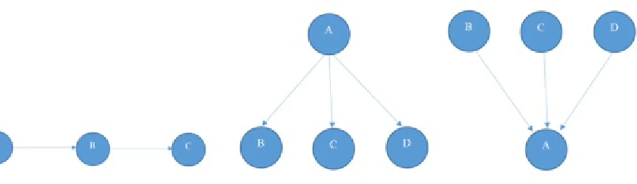
There are three basic causal networks should be introduced before starting the Bayesian net-works. According to Jensens’ book (Jensen, 1996), they are serial connections, diverging con-nections and converging concon-nections. In these concon-nections, when there is a link connects the variable A to variable B then variable B is achildof variable A, and variable A is aparentof vari-able B. It is obvious that the certainty of varivari-able of parent would have the impact on the child and vice versa. If taking diverging connections as the example, when the certainty function of variable B is increasing, the certainty of variable A will increase inversely; the increased certainty of variable A is expected to have the increased certainty of variable C or D.
For the serial and diverging connection, when the variable V between variables A and B are given evidence, or neither V or descendants of V have received evidence for converging connection, then A and B are calledd-separated. If A and B are not d-separated then them are called as d-connected. For instance, in serial connections of Figure4.1, if variable B is given, then A and B are called as d-separated or independent. Similarly, B, C, D are d-separated given A in diverging connections, or B, C, D are independent when nothing known about A in converging connec-tions (Jensen,1996).
Bayesian network(BN), is the widely used method, dealing with representing uncertain
Figure 4.1: Serial, diverging and converging connections
edge of probabilistic systems in a variety of real-world problems. It can be expressed as the graphical representation which consists of a directed acyclic graph (DAG) formed by variables together with the directed edges and conditional probability table (CPT) for conditional prob-abilities of variables on all corresponding parents (Jensen,1996). The connected nodes means that they are conditional dependent on the parent nodes, where the nodes that are not con-nected are conditionally independent of each other. It means if there are variables or nodes without any parent then they are called as theroot nodesand the unconditional probabilities or prior probabilitiesfor such variables should be specified.
Variables in a model which are neither hypothesis variables nor information variables are called mediating variables. Usually mediating variable will increase the precision of model, but there is a risk of increasing the complexity.
The quantitative analysis of BNs relies on the conditional independence assumption and causal dependence between nodes by developing the CPT for each node. The marginal posterior prob-ability P(X|E) for each variable X can be computed by using different classes of algorithms, where a set of variable E called as evidence, which means that the condition or the observation of variables is known. Then for the joint probability distribution of a set of variables [X1,X2...Xn],
it gives as follows, whereP[Xi] states for the parent of variableXi:
P[X1,X2...Xn]= n
Y
i=1
P[Xi|P(Xi)] (4.1)
The quantitative analysis of BNs can be both forward (or predictive) analysis and backward (or diagnostic) analysis. In forward analysis, the probability calculation of occurrence of any node is based on the prior probabilities of the root nodes and the conditional dependence of each node,
Table 4.1: Conditional probability of P (A|B)
b1 b2 b3
a1 0.2 0.3 0.1
a2 0.2 0.3 0.2
a3 0.6 0.4 0.7
Table 4.2: Joint probability for variables A and B
b1 b2 b3
a1 0.06 0.09 0.04
a2 0.06 0.09 0.08
a3 0.18 0.12 0.28
where root nodes are the nodes without parent nodes. In the backward analysis, the calculation of the posterior probability of any given set of variables given some evidence is considered as the instantiation of some of the variables to one of their admissible values (Bobbio et al.,2001).
4.1.2 Probability Calculation of Bayesian network
Conditional probabilityis the basic concept in Bayesian causal networks. It gives that the state-ment of probability of event A isP(A|B) given the event B. The basic rule for conditional proba-bility calculation isP(A|B)×P(B)=P(A,B), where theP(A,B) states for the probability of joint event of A and B. And this formula can also be read asP(A|B)×P(B) =P(B|A)×P(A) and this yields the wellBayes’ rule.
When the variable A has statesa1,a2...anand variable B has statesb1,b2...bnthen the probabil-ity distributions of variable A and B areP(A)=(a1,a2...an) andP(B)=(b1,b2...bn) respectively, wherePn
i=1ai =1 and Pn
j=1bj =1 . Then the basic rule could be apply for calculate the joint
probability and conditional probability for variable A and B. In Table4.1for conditional proba-bility ofP(A|B), we firstly assign the conditional probability of variables A and B, and it can be easily found that the sum of each column is equal to 1. Then if P (B) = (0.3, 0.3, 0.4), we can get Table4.2for joint probability of variables A and B by using basic rule, and we can summarize the P(A)=Pn
i=1(ai,bj)=(0.19, 0.23, 0.58). Similarly in Table4.3, the conditional probability P (B|A)
can be calculated by applying Bayes’ rule in4.1, where P (B) = (0.3, 0.3, 0.4) and P (A) = (0.19, 0.23, 0.58).
Table 4.3: Conditional probability of P (B|A)
b1 b2 b3
a1 0.32 0.26 0.31
a2 0.47 0.39 0.21
a3 0.21 0.35 0.48
Table 4.4: States Identification of Example
Rain soon (true) It will rain soon
Rain soon (false) It will not rain soon
Cloudy weather (true) Cloudy
Non-cloudy weather (false) Not cloudy
Weather forecast reports rain (true) Weather forecast reports rain before Weather forecast reports rain (false) Weather forecast don’t reports rain before
High humidity (true) humidity increase
High humidity (false) Feeling that humidity is normal as usual
4.1.3 Building Bayesian Network Model
There are generally three steps for organizing the BBN model: • Identify the hypothesis event
• Provide information variables for certainty estimation
• Build up causal structure after identifying the relationships between variables.
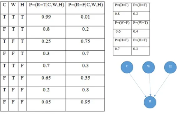
To explain how to build a Bayesian model, here is a simple example starting with two hypothesis events, namely‘rain soonand‘no rain soon. Therefore, the hypothesis variable (child) is called as R-soon (rain soon) with states y and n. Then three information variables (parents) are defined as C (Cloudy), W (weather forecast reports rain), H (high humidity) with two states y and n, which will indicate the child variables or be influenced and impacted by child variables. Then the states for all variables are shown in the Table4.4, in this example, only binary states (true and false) are assigned. Finally, we can estimate simple conditional probability for each variable by subjective estimation based on experience in Figure4.2.
Noted conditional probability table in this example is relatively small since only three variables with two states have been assigned. In the large-scale BBN model within numerous compo-nents, the CPT would enlarge geometrically and the increasing interactions between
subsys-Figure 4.2: Causal networks with probabilities for example Table 4.5: Posterior probability for child variable when Pr (R=T) =1
Pr(F) Pr(T) Variable C 0.7612 0.2388 Variable W 0.1985 0.8015 Variable H 0.5940 0.4060
tems will become too cumbersome to be involved in the computation. Then some software ap-plications are suggested to estimating the probabilities and implement computational model, such as (HUGIN,2015) suggested by (Jensen,1996). In this paper, the software (Matlab,2014) is suggested to be used in computational model.
We can get the marginalized probability of event R by computational software Matlab. Then the probability of event R occurs isP r(R=T)=0.3828, where the correspondingP r(R=F)=
0.6172, which means that the probability of raining soon is 38.28%. Moreover, the diagnostic analysis can be performed by computing the marginal probability of all parent variables when the evidence is given that it will rain soon. Then the posterior probabilities of parent variables when the evidence of R is given are shown in Table4.5and Table4.6.
Table 4.6: Posterior probability for child variable when Pr (R=F) =1 Pr(F) Pr(T)
Variable C 0.8241 0.1759 Variable W 0.8490 0.1510 Variable H 0.7657 0.2343
Table 4.7: Joint probability for example(C,W,H,R)
C W H R Values 1 1 1 1 0.3326 2 1 1 1 0.0672 1 2 1 1 0.0560 2 2 1 1 0.0168 1 1 2 1 0.1008 2 1 2 1 0.0234 1 2 2 1 0.0192 2 2 2 1 0.0012 1 1 1 2 0.0034 2 1 1 2 0.0168 1 2 1 2 0.1680 2 2 1 2 0.0392 1 1 2 2 0.0432 2 1 2 2 0.0126 1 2 2 2 0.0768 2 2 2 2 0.0228
From the second column of Table4.5, it can be found out that the posterior probabilities of Pr (C=T) =0.2388, Pr (W=T) =0.8015, Pr (H=T) =0.4060, which means that the severity rank of par-ent variables is: W>H>C. According to the first column in Table4.6, the severity rank of parent variables when there is no rain follows the similar rule, but this relationship is not revealed dis-tinctly. In addition, the joint probability could be also computed by Matlab, where the sum of values in Table4.7is equal to 1.
4.2 Comparison between Bayesian Network and other methods
In the past, Bayesian network is generally used in development of the artificial intelligence and industrial engineering decision making strategy (Jensen,1996), since this method can deal with the error and uncertainty in probabilistic computation model when lacking of statistical data for
prior probability estimation. Recently, due to the ability of information updating for Bayes’ the-orem, Bayesian network was starting to be applied in the reliability assessment of large complex system, such as software-based system (Gustav,2000), simple structural system (Sankaran et al., 2001) or as an alternative for traditional reliability assessment method (Bobbio et al., 2001). However, so far few researchers have performed the reliability assessment in the subsea BOP system.
There are many traditional reliability assessment methods, such as reliability block diagram (RBD), fault tree analysis and event tree analysis. Similar as Bayesian Network, these methods are developed based on the description of the system flow chart of system functions. Compared to those methods, however, Bayesian Network can update the system information or perform the reassessment of reliability when the test data of system or components becomes available. It is one of the biggest differences between the other methods and Bayesian Network: when infor-mation or observations are provided for some nodes or the whole system, also called as “given evidence”, it can “renew” the performance assessment of any other components or the whole system, which is impossible to obtain by all these methods.
There are some other advanced methods for reliability assessment, like Markov method or Petri-net method, and they are generally used in dynamic analysis of the complex system. However, one of the difficulties is that the reliability engineers should identify all the possible states before building the model. It may be hard for the expert of reliability engineering but who is unfamiliar with the specific system.
4.3 From Fault Tree Analysis to Bayesian Network
In this section, FTA is the one analytically compared to BN by investigating how FTA can be translated into BN without losing any details and obtaining the advanced modelling power si-multaneously,and the unreliability of the top event (TE) or subsystem of FTA can be also cal-culated as the prior probability of target variable in faulty state when given no evidence in BN model, while backward (diagnostic) analysis can also compute the severity ranking of compo-nents. Basically, FTA can be analyzed both qualitatively and quantitatively, and minimal cut-sets method is most frequently used in quantitative part.
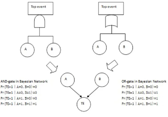
Figure 4.3: AND-gate and OR-gate in Bayesian Network
Compared to FTA which is the mostly applied method in reliability assessment of subsea BOP system in the past decades, BN model can avoid generating duplication of basic nodes or events, which reduce the model size and make the system more easily to be understood, especially in the large and complex system with many components and complicated interrelation between components. Moreover, some unnecessary assumptions in FTA can be removed when trans-lating into BN: (1) the binary gates (AND gate and OR gate) are replaced by the probabilistic gates; (2) the general binary states (survival or failure) for components in FTA are extended to be multiple states in BN; (3) components are no longer statistically independent.
FTA can be translated by an algorithm (Bobbio et al., 2001) or automatically by the software named RADYBAN (Cai et al., 2012a). Kim(2011) also provides the method for mapping RBD into BN. Here taking the algorithm method as the example to show how the AND-gate and OR-gate could be translated into BN nodes.
As Figure4.3shown above, we have two basic events A and B, where the value 0 and 1 represent non-fault state and fault state, respectively. It is noticed that the translation of AND-gate and OR-gate from FTA results in the same DAG in BBN but with the different corresponding CPTs.