Abstract²The objective of this paper is to compare the time specification performance between conventional controller PID and modern controller SMC for an inverted pendulum system. The goal is to determine which control strategy delivers better performance with UHVSHFW WR SHQGXOXP¶V DQJOH DQG FDUW¶V SRVLWLRQ 7KH LQYHUWHG pendulum represents a challenging control problem, which continually moves toward an uncontrolled state. Two controllers are presented such as Sliding Mode Control (SMC) and Proportional-Integral-Derivatives (PID) controllers for controlling the highly nonlinear system of inverted pendulum model. Simulation study has been done in Matlab Mfile and simulink environment shows that both controllers are capable to control multi output inverted pendulum system successfully. The result shows that Sliding Mode Control (SMC) produced better response compared to PID control strategies and the responses are presented in time domain with the details analysis.
.
Keywords²SMC, PID, Inverted Pendulum System. I. INTRODUCTION
The one-dimensional inverted pendulum is a nonlinear problem, which has been considered by many researchers (Omatu and Yashioka, 1998; Magana and Holzapfel, 1998; Nelson and Kraft, 1994; Anderson, 1989), most of which have used linearization theory in their control schemes. In general, the control of this system by classical methods is a difficult task (Lin and Sheu, 1992). This is mainly because this is a nonlinear problem with two degrees of freedom (i.e. the angle of the inverted pendulum and the position of the cart), and only one control input [1]. The inverted pendulum is used for control engineers to verify a modern control theory since its characteristics as marginally stable as a control. This system is popularly known as a model for the attitude control especially in aerospace field. However, it also has its own deficiency due to its principles; highly non-linear and open-loop unstable system [2]. Thus, causing the pendulum falls
A.N.K. Nasir is with Faculty of Electrical & Electronics Engineering, Universiti Malaysia Pahang, Pekan Pahang Malaysia (phone: 609-4242145-; fax: 609-424-2035; e-mail: kasruddin@ ump.edu.my).
R.M.T. Raja Ismail is with Faculty of Electrical & Electronics Engineering, Universiti Malaysia Pahang, Pekan Pahang Malaysia (e-mail: [email protected]).
M.A. Ahmad is with Faculty of Electrical & Electronics Engineering, Universiti Malaysia Pahang, Pekan, Pahang, Malaysia (e-mail: [email protected]).
over quickly whenever the system is simulated due to the failure of standard linear techniques to model the non-linear dynamics of the system. Moreover, it makes the identification and control become more challenging [3]. The mathematical model is established through a modeling process where the system is identified based on the conservation laws and property laws. This process is crucial since a controller is design solely based on this mathematical model. Thus, an accurate equation must be derived in order for the controller to response accordingly.
The common control approaches to overcome the problem by this system namely linear quadratic regulator (SMC) control and PID control that require a good knowledge of the system and accurate tuning to obtain good performance. Nevertheless, it attribute to difficulty in specifying an accurate mathematical model of the process [4]. This paper presents investigations of performance comparison between conventional (PID) and modern control (SMC) schemes for an inverted pendulum system. The dynamic model and design requirement have been taken from Carnegie Mellon, University of Michigan [5]. Performance of both control VWUDWHJ\ZLWKUHVSHFWWRSHQGXOXP¶VDQJOHDQGFDUW¶VSRVLWLRQ is examined. Comparative assessment of both control schemes to the system performance is presented and discussed.
II.DYNAMIC MODEL
Modeling is the process of identifying the principal physical dynamic effects to be considered in analyzing a system, writing the differential and algebraic equations from the conservative laws and property laws of the relevant discipline, and reducing the equations to a convenient differential equation model [6]. This section provides a brief description on the modeling of the inverted pendulum system, as a basis of a simulation environment for development and assessment of both control schemes. The system consists of an inverted pole hinged on a cart which is free to move in the x
direction as shown in Fig. 1.
In order to obtain the dynamic model of the system, the following assumptions have been made:
1) The system starts in a state of equilibrium meaning that the initial conditions are therefore assumed to be zero.
Performance Comparison between Sliding
Mode Control (SMC) and PD-PID Controllers
for a Nonlinear Inverted Pendulum System
2) The pendulum does not move more than a few degrees away from the vertical to satisfy a linear model.
3) A step input is applied to the position of the cart.
Fig. 1 Cart and Inverted Pendulum System
The parameters of the inverted pendulum system used for the experiment are shown in Table I.
Fi g. 2 shows the free body diagram of the cart and inverted pendulum system. From the free body diagram, the following dynamic equations in horizontal direction in (1) and vertical direction in (2) are determined.
F ml ml x b x m M ) TcosT T sinT ( 2 (1) T T T sin cos ) (Iml2 mgl mlx (2)
Fig. 2 Free body diagram of cart and inverted pendulum The dynamic equations in (1) and (2) should be linearized about ș ʌ. After linearization, the dynamic equations (3) and (4) are obtained, i.e.
x ml mgl ml I )I I ( 2 (3) u ml x b x m M ) I ( (4)
By manipulating the dynamics equations in (3) and (4), and substituting the parameter values of the cart and pendulum, the IROORZLQJ WUDQVIHU IXQFWLRQ RI WKH SHQGXOXP¶V DQJOH DQG WUDQVIHU IXQFWLRQ RI FDUW¶V SRVLWLRQ DUH REWDLQHG DV VKRZQ LQ (5) and (6) respectively. 4545 . 4 1818 . 31 1818 . 0 5455 . 4 ) ( ) ( 2 3 ) s s s s s u s (5) 4545 . 4 1818 . 31 1818 . 0 5455 . 44 8182 . 1 ) ( ) ( 2 3 s s s s s u s x (6)
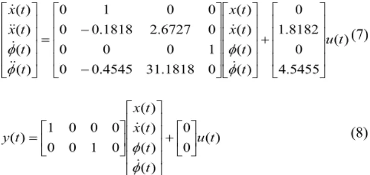
The transfer functions can be represented in state±space form and output equation as stated in (7) and (8)
) ( 5455 . 4 0 8182 . 1 0 ) ( ) ( ) ( ) ( 0 1818 . 31 4545 . 0 0 1 0 0 0 0 6727 . 2 1818 . 0 0 0 0 1 0 ) ( ) ( ) ( ) ( t u t t t x t x t t t x t x » » » » ¼ º « « « « ¬ ª » » » » ¼ º « « « « ¬ ª » » » » ¼ º « « « « ¬ ª » » » » ¼ º « « « « ¬ ª I I I I (7) ) ( 0 0 ) ( ) ( ) ( ) ( 0 1 0 0 0 0 0 1 ) ( u t t t t x t x t y » ¼ º « ¬ ª » » » » ¼ º « « « « ¬ ª » ¼ º « ¬ ª I I (8)
From (7), the stability of the system can be determined by calculating the open-loop poles using
0 )
det(sIA (9)
where A is a system matrix. By solving (9), the open-loop poles are determined as follows:
Open-loop poles: 0 ±0.1428 5.5651 ±5.6041
Open loop system poles shows that one of the four poles, 5.5651 lies on right hand side of the s-plane which stated that the system is unstable. Therefore, a controller has to be designed in order to stabilize the inverted pendulum system. As can be seen from (1) and (2), all nonlinear terms remain in the equations. All these nonlinear equations are used to design the proposed SMC and PID controllers which will be described in details in section III.
III. CONTROLLER DESIGN & SIMULATION In this section, two control schemes Sliding Mode Control and PD-PID are proposed and described in detail. The following design requirements have been made to examine the performance of both control strategies.
1) The system overshoot (%OS) of cart position, x is to be at most 10%.
2) The system overshoot (%OS) of SHQGXOXP¶V angular position, T is to be at most 33 degrees or 0.58 radians. 3) The rise time (Tr) of FDUW¶Vposition, x less than 5 s.
TABLEI
PARAMETERSOFTHEINVERTEDPENDULUMSYSTEM Symbol Parameter Value Unit
M Mass of the cart 0.5 kg m Mass of the pendulum 0.5 kg B Friction of the cart 0.1 N/m/s L Length of the pendulum 0.3 m
I Inertia of the pendulum 0.006 kgm2
4) The settling time (Ts) RIFDUW¶V position, x and SHQGXOXP¶V angle ș is to be less than 5 seconds.
5) Steady-state error is within 2% of the desired value.
A.PID Controller
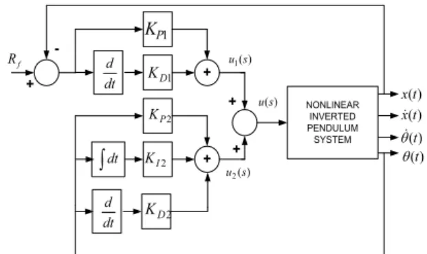
PID stands for Proportional-Integral-Derivative [7]. This A common strategy in the control of an inverted pendulum system involves the utilization of PID feedback of collocated sensor signals. PID is a type of feedback controller whose output, a control variable (CV), is generally based on the error (e) between defined set point (SP) and some measured process variable (PV). Each element of the PID controller refers to a particular action taken on the error. In order to demonstrate the performance of the PID controller in locating the inverted pendulum to its desired position and angle, the collocated sensor signal of the position of the cart about x-axis, x(s) and angular position of the pendulum about y-axis ș(s) are fed back and compared to the reference position, xf(s) and angle
șf(s)respectively. In this work, such a strategy is adopted at this stage. A sub-block diagram of the PID controller is shown in Fig. 3, where KP, KI and KD are proportional, integral and derivative gains, respectively. xand x represent horizontal position and velocity of the cart, respectively, T and T represent swing angle and swing velocity, respectively Rf is the reference horizontal cart position. In this study, PD controllers are required to control the position of the cart on the x-axis and PID controller is required to control the pendulum angular position Tabout the y-axis. The cart position error is regulated through the proportional and derivative gain PD and pendulum angular position error is regulated through the proportional, integral and derivative gain PID. In Fig. 3 u(s) represent the control torque to control the motor on the cart. The control signal u1(s) and u2(s) represent the controller outputs of PD and PID controllers and can be represented as (10) and (11) respectively:
)] ( ) ( [ ) ( 1 1 1 position PID K s r s r s s K K s u I D f P ¸ ¹ · ¨ © § (10) )] ( ) ( [ ) ( 2 2 2 angle PID K s s s s K K s u D f I P ¸T T ¹ · ¨ © § (11)
where s is the Laplace variable. Hence the closed-loop transfer function is obtained as (12) and (13).
) ( 1 ) ( ) ( ) ( 1 1 1 1 1 1 s G s K s K K s G s K s K K s r s r I D P I D P f ¸ ¹ · ¨ © § ¸ ¹ · ¨ © § (12) ) ( 1 ) ( ) ( ) ( 2 2 2 2 2 2 s G s K s K K s G s K s K K s s I D P I D P f ¸ ¹ · ¨ © § ¸ ¹ · ¨ © § T T (13)
In this paper, the Ziegler-Nichols approach is utilized to design both PID controllers. Analyses the tuning process of the proportional, integral and derivative gains using Ziegler-Nichols technique shows that the optimum response of PID controller for controlling cart position is achieved by setting
KP1= 10, and KD1= 6,while for controlling pendulum angular position, KP2 = ±9,KI2 = 0.01 and KD2 = 0.01. All the PD and PID controller parameters must be tuned simultaneously to achieve the best responses as desired.
-+ NONLINEAR INVERTED PENDULUM SYSTEM ³dt + ) (t x ) (t x ) (t T(t) T f R dt d + + + dt d ) ( 1s u ) ( 2s u ) (s u 1 P K 1 D K 2 P K 2 I K 2 D K
Fig. 3 Block diagram of PD-PID controller and Nonlinear Inverted Pendulum System
B.Sliding Mode Controller (SMC)
SMC is a method in modern control theory that uses state-space approach to analyze such a system. Using state-state-space methods it is relatively simple to work with a multi-output system [8].The typical structure of a sliding mode controller (SMC) is composed of a nominal part and additional terms to deal with model uncertainty. The way SMC deals with uncertainty is to drive the plants state trajectory onto a sliding surface and maintain the error trajectory on this surface for all subsequent times. The advantage of SMC is that the controlled system becomes insensitive to system disturbances. The sliding surface is defined such that the state tracking error converges to zero with input reference. With the perspective to achieve zero steady state error, Cao and Xu (2001) and Sam et al. (2002) have proposed the proportional integral sliding mode control (PISMC) in their studies [9]. The proportional factor in this controller gives more freedom in selecting some parameters matrices that will make the output response faster and the stability condition to be more easily satisfied. The proportional integral sliding surface equation can be represented as (14).
>
@
W W V t Sxt SA SBKx d t³
0 ) ( ) ( ) ( (14)where xnis a vector of measureable states, Anxn, m
B and Smxnare constant matrices. Kmxnis a constant matrix such that the matrix (A+BK) is asymptotically stable and has the stable eigenvalues. The system can be stabilized using full state feedback. The schematic of this type of control system is shown in Fig. 4.
+ NONLINEAR INVERTED PENDULUM SYSTEM ) (t x ) (t x ) (t T ) (t T f R u(s) Sliding Mode Controller
-Fig. 4 The SMC control structure
The control law should be designed such that the reaching condition V(t)V(t)0 is satisfied [10]. This criterion should be fulfilled to ensure that the state will move toward and reach the chosen sliding surface. The equivalent control method will be used for finding equations of ideal sliding mode. In this technique a time derivative of the sliding surface V(t)along the system trajectory is set equal to zero, and the resulting algebraic system is solved for the equivalent control. The control law that will be implemented into this system is presented as (15). ) ( ) ( ) (t u t ut u eq ' (15)
where ueq(t)is the equivalent sliding mode control and continuous function 'u(t)is added to satisfy reaching condition. ueq(t)and 'u(t)is a and can be represented as (16) and (17). ) ( ) (t Kxt ueq (16) (16) c t t SB t u G V UV ' ) ( ) ( ) ( ) ( 1 (17) (17)
where Gcis the boundary layer thickness and Uis a design parameter. For this study, the values for controller parameters are tabulated in Table II. All these parameters must be substituted into (16) and (17).
IV. RESULT AND ANALYSIS
In this section, the simulation results of the proposed controller, which is performed on the model of an inverted pendulum system, are presented. Comparative assessment of both control strategies to the system performance are also discussed in details in this section.
Nonlinear inverted pendulum system with SMC and PID controller block diagram produced two responses, angular position ș and linear position x. As stated earlier, the desired value of the cart position x of the inverted pendulum system was set to move one meter. It means that the cart needs to move from initial position to one meter away and at the same WLPHWKHSHQGXOXP¶s angle must eliminate the angular position șWR]HURUDGLDQVVRWKDWSHQGXOXP¶VURGLVYHUWLFDOO\VWUDLJKW
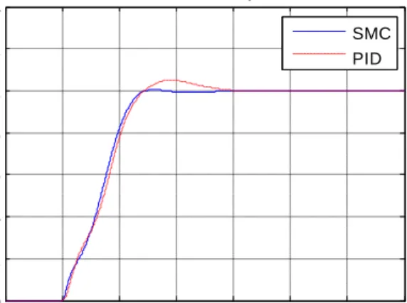
Fig. 5 shows the comparison of the inverted pendulum system cart position response between SMC and PID controller graphically.
Fig. 5 Nonlinear Inverted Pendulum Cart Position Response In this figure, the response for the cart position of the system with SMC controller is represented by straight line or blue color line and the response for the cart position of the inverted pendulum with PD-PID controller is represented by dotted line or red color line. Fig. 5 shows that both of the controllers are capable to control the cart position of the nonlinear inverted pendulum system.
Table III shows the summary of the performance characteristics of the inverted pendulum cart position between SMC and PID controller quantitatively. Based on the data tabulated in Table III, SMC has the fastest settling time of 2.33 seconds while PID has the slowest settling time of 3.52 seconds. An extra of 1.19 seconds is required for the PID controller to move the cart to one meter away from its original position. Similarly, for the percentage maximum overshoot, SMC controller has the smallest percentage overshoot 0.5 %. The maximum displacement of the cart when SMC control signal applied to the system is 1.005 meters while maximum displacement of the balancing robot when PID control signal applied to the system is 1.05 meters. A difference distance of minimum 0.045 meters is required for the PID controller to stabilize cart to desired position. The proposed SMC and PID controllers are able to balance cart to the desired position with low percentage overshoot. In term of the rise time, inverted pendulum with SMC controller has the fastest rise time 1.01 seconds while inverted pendulum with PID controller needs an extra time of 0.01 seconds to rise from 10% to the 90% of the initial value. In term of steady state error, both of the controllers had shown very outstanding performance by giving zero error at time 5 seconds and more. The responses of the inverted pendulum cart position on x axis have acceptable minimum overshoot and undershoot.
Fig. 6 shows the inverted pendulum with SMC and PID controller pendulum angular position responses. It shows that the result has got similar pattern and not much difference to 7KH LQLWLDO YDOXH RI WKH SHQGXOXP¶V DQJXODU
0 1 2 3 4 5 6 7 0 0.2 0.4 0.6 0.8 1 1.2 1.4 Time (second) C a rt P o s it io n ( m e te r)
Cart Position Response
SMC PID
position is zero radians. The pendulum needs to balance itself by eliminating the angular position ș VRWKDW WKHSHQGXOXP¶V rod remains vertically straight in upright position. Fig. 6 shows that both of the SMC and PID controllers are capable of controlling the nonlinear unstable inverted pendulum angular position. Table IV shows the summary of the performance characteristics of the inverted pendulum angular position between SMC and PID controller quantitatively.
Based on the data tabulated in Table IV, PID has the fastest settling time of 2.93 seconds while SMC has the slowest settling time of 3.03 seconds. An extra time of 0.1 seconds is UHTXLUHGIRUWKH60&FRQWUROOHUWREDODQFHSHQGXOXP¶VURGLQ vertical upright position. In contrast, for the maximum undershoot, SMC controller has the best overshoot which is the lowest overshoot between two controllers.
7KH PD[LPXP DQJXODU GLVSODFHPHQW RI WKH SHQGXOXP¶V URG when SMC control signal applied to the system is 0.50 radians ZKLOHPD[LPXPDQJXODUGLVSODFHPHQWRIWKHSHQGXOXP¶VURG when PID control signal applied to the system is 0.55 radians. An extra angle of minimum 0.05 meters is required for the PID controller to balance pendXOXP¶VURGWRGHVLUHGSRVLWLRQ compared to SMC controller. Despite the large initial values for the displacement, the proposed SMC and PID controllers are able to bring thH SHQGXOXP¶V URG to the vertical upright position. ,QWHUPRIWKHULVHWLPHSHQGXOXP¶VURGZLWK60& controller has the fastest rise time 0.14 seconds while SHQGXOXP¶V URG ZLWK 3,' FRQWUROOHU QHHGV DQ H[WUD WLPH RI 0.02 seconds to rise from 10% to the 90% of the initial value. In term of steady state error, both of the controllers had shown very outstanding performance by giving zero error at time 5 seconds and more. The responses of the inverted pendulum angular position have acceptable overshoot and undershoot. Performance characteristics for linear and angular position represented in bar chart form are shown in Fig. 7 and Fig. 8 respectively.
Fig. 6 1RQOLQHDU,QYHUWHG3HQGXOXP3HQGXOXP¶VAngular Position Response
Fig. 7 Performance characteristics for cart position
Fig. 8 Performance characteristics for pendulum position
0 1 2 3 4 5 6 7 -0.4 -0.2 0 0.2 0.4 0.6 Time (second) P e n d u lu m 's A n g le ( ra d ia n s )
Pendulum's Angle Response
SMC PID 1.01 2.33 0.50 1.02 3.52 5.00 0 1 2 3 4 5 6 Tr Ts OS SMC PID 0.14 3.03 0.5 0.16 2.93 0.55 0 0.5 1 1.5 2 2.5 3 3.5 Tr Ts OS SMC PID TABLEIII
SUMMARY OF PERFORMANCE CHARACTERISTICS OF THE INVERTED
PENDULUM CART POSITION BETWEEN SMC AND PID
Time Response
Spesification SMC PID
Rise Time 1.01 sec 1.02 sec Settling Time 2.33 sec 3.52 sec Steady state error 0.00 0.00
Percentage Max. overshoot
0.5 % 5 %
TABLEIV
SUMMARY OF PERFORMANCE CHARACTERISTICS OF INVERTED
PENDULUM ANGULAR POSITION BETWEEN SMC AND PID
Time Response
Spesification SMC PID
Rise Time 0.14 sec 0.16sec
Settling Time 3.03 sec 2.93 sec Steady state error 0.00 0.00 Maximum overshoot 0.50 radians 0.55 radians
V.CONCLUSION
In this paper, two controllers such as SMC and PID are successfully designed. Based on the results and the analysis, a conclusion has been made that both of the control method, modern controller (SMC) and conventional controller (PID) are capable of controlling the nonlinear inverted pendulum system angular and linear position. All the successfully designed controllers were compared. The responses of each controller were plotted in one window and are summarized in Table III and Table IV. Simulation results and bar charts in Fig. 7 and Fig. 8 show that SMC controller has better performance compared to PID controller in controlling the nonlinear inverted pendulum system. Further improvement need to be done for both of the controllers. PID controller should be improved so that the maximum overshoot and maximum undershoot for the linear and angular positions do not have very high range as required by the design criteria. On WKH RWKHU VLGH /45 FRQWUROOHU FDQ EH LPSURYHG VR WKDW LW¶V settling time for angular position might be reduced as faster as PID controller.
REFERENCES
[1] A. Ghanbarie and M. Farrokhi,³Decentralized decoupled sliding-mode control for two-dimensional inverted pendulum using neuro-fuzzy modeling,´Proc. of IEEE Int. Conf. on Engineering of Intelligent Systems, pp. 1-6, Sept. 2006.
[2] Q.-R. Li, W.-H. Tao, N. Sun, C.-Y. Zhang and L.-+<DR³6WDELOL]DWLRQ FRQWURORIGRXEOHLQYHUWHGSHQGXOXPV\VWHP´Proc. of 3rd Int. Conf. on Innovative Computing, Information and Control, pp. 417-420, 2008. [3] - ;LH ; ;X DQG . ;LH ³0RGHOOLQJ DQG VLPXODtion of the inverted
SHQGXOXP EDVHG RQ JUDQXODU K\EULG V\VWHP´Proc. of Control and Decision Conf., pp. 3795-3799, 2008.
[4] W. J. Chen, L. Fang and K. K. Lei, ³Fuzzy logic controller for an inverted pendulum system´ Proc. of IEEE Int. Conf. on Intelligent Processing Systems, pp. 185-189, Oct. 1997.
[5] Carnegie Mellon, University of Michigan. [Online]. Available: http://www.engin.umich.edu/group/ctm.
[6] M. Y. Sam, J. H. S. Osman and R. A. Ghani ³Proportional integral sliding mode control of a quarter car active suspension,´Proc. of IEEE Region 10 Conf. on Computers, Communications, Control and Power Engineering, vol. 3, pp. 1630-1633, Oct. 2002.
[7] N. S. Nise, Control System Engineering. New York: John Wiley & Son, 2000.
[8] A. N. K. Nasir, M. A. Ahmad and 0 ) 5DKPDW ³3HUIRUPDQFH comparison between LQR and PID controller for an inverted pendulum system,´Proc. of Int. Conf. on Power, Control and Optimization, vol. 1052, pp. 124-128, Oct. 2008.
[9] M. F. Abdollah, ³3URSRUWLRQDO,QWHJUDO6OLGLQJ0RGH&RQWUROof A Two-:KHHOHG %DODQFLQJ 5RERW´ 0DVWHU¶V thesis, Faculty of Electrical Engineering, Universiti Teknologi Malaysia, 2006.
[10] C. Edwards and S. K. Spurgeon, Sliding Mode Control: Theory and Applications. London: Taylor & Francis, 1998.