ANALYSIS OF PLATOON IMPACTS ON LEFT-TURN DELAY AT UNSIGNALIZED INTERSECTIONS
A Thesis by FENG WAN
Submitted to the Office of Graduate Studies of Texas A&M University
in partial fulfillment of the requirements for the degree of MASTER OF SCIENCE
December 2010
Analysis of Platoon Impacts on Left-Turn Delay at Unsignalized Intersections Copyright 2010 Feng Wan
ANALYSIS OF PLATOON IMPACTS ON LEFT-TURN DELAY AT UNSIGNALIZED INTERSECTIONS
A Thesis by FENG WAN
Submitted to the Office of Graduate Studies of Texas A&M University
in partial fulfillment of the requirements for the degree of MASTER OF SCIENCE
Approved by:
Chair of Committee, Yunlong Zhang Committee Members, Dominique Lord
Clifford Spiegelman
Head of Department, John Niedzwecki
December 2010
ABSTRACT
Analysis of Platoon Impacts on Left-Turn Delay at Unsignalized Intersections. (December 2010)
Feng Wan, B.S., Tongji University
Chair of Advisory Committee: Dr. Yunlong Zhang
Traffic platoons created by traffic signals may have impacts on the operations of downstream intersections because they change the arrival pattern and gap distribution of upstream traffic. There’s been a lot of research dealing with platoon effects on
operations at signalized intersections, while very limited research has been done for that of unsignalized intersections.
This research aims to develop a methodology for analyzing the platoon impacts on major-street left-turn (MSLT) delay at two-way stop-controlled (TWSC)
intersections. The main idea is using a microscopic simulation tool to simulate different platoon scenarios in opposing through traffic, then applying regression models to capture the impacts of platoons on the delay of MSLT. Two platoon variables were adopted as a simplification of the complex platoon scenarios, making it practical to analyze the platoon effects on MSLT delay.
The first two steps were to build simulation models for real-world unsignalized intersections and simulate scenarios with a combination of various factors related to platoons in VISSIM simulation. Calibrations of these simulation models based on field
data were performed before simulation started. The next step was to define, derive and calibrate two platoon variables for describing the duration and intensity of platoon arrivals in the opposing through traffic, which effectively simplified the large
combination of various factors. At last, the two platoon variables and their relationship with MSLT delay change factor were modeled with regression tools. A relationship between the two variables and the delay change factor was established, which indicated a positive effect by upstream platoons on MSLT delay and made it possible to quantify the impacts. The findings in this research could also be used for future research on left-turn treatment regarding platoon or signal impacts.
DEDICATION
ACKNOWLEDGEMENTS
I would like to thank my committee chair, Dr. Yunlong Zhang, my committee members, Dr. Dominique Lord and Dr. Clifford Spiegelman, for their guidance and support throughout the course of this research. I’d like to thank Dr. Kay Fitzpatrick for providing the opportunity to work on the NCHRP project and for providing data for this thesis work.
The data used in this research is from the National Cooperative Highway
Research Program (NCHRP) project 3-91, “Left-Turn Accommodations at Unsignalized Intersection.” The research is sponsored by the American Association of State Highway and Transportation Officials (AASHTO), in cooperation with the Federal Highway Administration (FHWA), and is conducted in the National Cooperative Highway Research Program, which is administered by the Transportation Research Board of the National Research Council. I really appreciate the efforts of the numerous staff and student workers who collected and reduced the NCHRP 3-91 data used in this research.
Thanks also go to my friends and colleagues and the department faculty and staff for making my time at Texas A&M University a great experience.
Finally, thanks to my mother and father for their encouragement and to my wife for her patience and love.
The opinions and conclusions expressed or implied in this paper are those of the authors. They are not necessarily those of the Transportation Research Board, the National Research Council, the Federal Highway Administration, the American
Association of State Highway and Transportation Officials, or the individual states participating in the National Cooperative Highway Research Program.
NOMENCLATURE
AWSC All-Way Stop-Controlled
LOS Level-of-Service
LTL Left-Turn Lane
MOE Measure-of-Effectives
MSLT Major-Street Left-Turn
TWSC Two-Way Stop-Controlled
TABLE OF CONTENTS Page ABSTRACT ... iii DEDICATION ... v ACKNOWLEDGEMENTS ... vi NOMENCLATURE ... viii TABLE OF CONTENTS ... ix LIST OF FIGURES ... xi
LIST OF TABLES ... xii
CHAPTER I INTRODUCTION ... 1
Background ... 1
Statement of Problem ... 2
Purpose of the Study ... 3
Organization of the Thesis ... 3
II LITERATURE REVIEW ... 5
Platoon Effect ... 5
Left-turn Operations ... 8
Critical Gap Calibration ... 10
Summary ... 12
III DATA COLLECTION ... 13
Field Data ... 13
Simulation Results ... 20
IV METHODOLOGY ... 22
CHAPTER Page
Simulation Scenarios Development ... 32
Platoon Variables Definition and Calibration ... 35
Delay Adjustment with Platoon Effects ... 40
V RESULTS ... 42
Critical Gap Calibration Results ... 42
Calibration of Platoon Variables from Derivation ... 48
Delay Adjustment Factors ... 50
VI CONCLUSIONS ... 61
VII LIMITATIONS AND FUTURE WORK ... 63
REFERENCES ... 64 APPENDIX A ... 67 APPENDIX B ... 71 APPENDIX C ... 74 APPENDIX D ... 77 VITA ... 79
LIST OF FIGURES
Page Figure 1 Harmelink – Left-Turn Warrant Graph
40 mph, 5% Left Turns, 1967 ... 9
Figure 2 Structure of Research Methodology ... 22
Figure 3 Steps in Research Methodology ... 23
Figure 4 Chart of Gap Acceptance Model ... 25
Figure 5 AZ-01 Raff's Critical Gap ... 27
Figure 6 Simulation Scenario Example ... 34
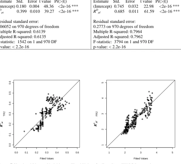
Figure 7 Simulated Platoon Variables vs. Fitted Values for Four-Lane TWSC Intersections ... 49
Figure 8 MSLT Delay Adjustment Factors vs. Values Fitted by Regression ... 53
Figure 9 3-D Plot of Delay Adjustment Factors for Four-Lane TWSC Intersections ... 55
LIST OF TABLES
Page
Table 1 Relationship between Arrival Type and Platoon Ratio (Rp)... 6
Table 2 Progression Adjustment Factor for Uniform Delay Calculation ... 7
Table 3 The 2000 HCM Critical Gaps and Follow-Up Times at TWSC Intersections ... 10
Table 4 Partial Information of Gap Acceptance ... 14
Table 5 Partial Information of Operation Data ... 16
Table 6 TWSC Intersection Characteristics ... 18
Table 7 Simulation Results ... 21
Table 8 Comparison of Raff’s and Logistic Method ... 31
Table 9 One Set of Upstream Traffic Signals ... 33
Table 10 Critical Gaps from Raff's and Logistic Regression Model ... 44
Table 11 Final Critical Gap Values for Each Intersection ... 45
Table 12 T Test for Factors Related to Critical Gaps ... 46
Table 13 Recommended Critical Gap Values ... 47
Table 14 Platoon Variables for Four-Lane TWSC Intersections ... 48
Table 15 Relationships between Simulated and Derived Parameters for Four-Lane TWSC Intersections ... 49
Table 16 Dataset of MSLT Fda for Two-Lane TWSC Intersections with LTL ... 51
Table 17 Regression Results for Platoon Variables and MSLT Delay Adjustment Factors ... 52
Page Table 18 Delay Adjustment Factors of MSLT Movement
for Four-Lane TWSC Intersections ... 56 Table 19 Comparison of Models for Four-Lane TWSC Intersections
with LTL ... 57 Table 20 Comparison of Models for Four-Lane TWSC Intersections
without LTL ... 58 Table 21 Delay Adjustment Factors of MSLT Movement
for Four-Lane TWSC Intersections with LTL ... 59 Table 22 Delay Adjustment Factors of MSLT Movement
CHAPTER I INTRODUCTION
Background
The left-turn movement at an intersection has always been a major issue for both traffic operation and safety of an intersection. At intersections with traffic volumes high enough to satisfy traffic signal warrants, traffic signals are often installed and left turn movements may be protected depending on the left-turn and opposing through volumes. At unsignalized intersections, left-turns are made safely only when sufficiently large gaps are present in opposing through traffic. Because of this, left-turn delay is common and left-turn operations are more restricted than other movements at unsignalized intersections.
In this research, the interest centers on the major-street left-turn (MSLT)
movement at a two-way stop-controlled (TWSC) intersection. The analysis of delay and other operational or safety variables are essential for the level-of-service (LOS) and safety performance at an unsignalized intersection. Left-turn delay is dependent upon left-turn and opposing through movement volumes, gap distributions, critical gaps, and intersection geometry. In addition to the demand levels of left-turn and opposing through movements, the arrival patterns of opposing through vehicles could also be a significant factor affecting left-turn delay because it changes the gap distribution.
____________
A traffic signal discharges vehicles primarily on green times, with vehicles often leaving the intersection on green in platoons. Platoons might have a significant impact on the gap distribution of through vehicles and further affect the MSLT movement delay at the downstream intersection. The effects of platoons generated from the upstream signal intersection on MSLT delay are investigated in this research. VISSIM simulation is selected as the platform for research and field data is used to calibrate VISSIM simulation.
In order to get reliable simulation results from VISSIM, the parameters should be carefully calibrated before performing the simulation. Delay calculations for left-turn movements at unsignalized intersections are based on gap acceptance theory in the 2000 Highway Capacity Manual [1], and critical gap and follow-up time are the two
fundamental parameters of the gap acceptance model. The calibration in this research was based on the extensive database established for the NCHRP 3-91 project, Left-Turn Accommodations at Unsignalized Intersections. 30 TWSC unsignalized intersections in three states of United States (Texas, Arizona, and New York) were videotaped with DV cameras, out of which useful data was extracted. Raff’s critical gap model and logistic regression model were employed to calibrate and analyze the critical gaps in this research.
Statement of Problem
As mentioned above, the platoons may have impacts on left-turn operations at the downstream unsignalized intersection. Particularly, the platoon effects on the delay to
the major-street left-turn movement at the downstream TWSC intersection will be investigated in this research. While unsignalized intersections include both two-way stop-controlled (TWSC) and all-way stop-controlled (AWSC) intersections, this research focuses on just the TWSC intersections. Very limited research has been done on this topic, and therefore further research is demanded.
Purpose of the Study
The objective of this research is to develop a methodology for estimating the platoon effects on the MSLT operations at TWSC intersections and provide
recommendations for left-turn treatment at unsignalized intersections. Goals to achieve include:
calibrating and updating critical gap values for the left-turn operation for unsignalized intersections,
designing analysis on the platoon impacts on MSLT delays,
developing the methodology for estimating the platoon effects, and
making recommendations on left-turn treatments based on the simulation results.
Organization of the Thesis
The paper is organized as follows. Chapter I gives a brief introduction to the research that will be performed. Chapter II describes documented literatures that are related to the analysis of platoon effects on left-turn delay at unsignalized intersections.
Chapter III briefs the datasets prepared in this research. Chapter IV is the methodology part, which includes the description of the data collection, approach of simulation and method of analysis. Chapter V and Chapter VI present the results and the main
conclusions of the research. Finally, limitations and future work are documented in Chapter VII.
CHAPTER II LITERATURE REVIEW
Platoon Effect
Traffic signals discharge queues on green time and cause vehicles to travel in platoons at the signalized intersection. Platooning traffic has quite different
characteristics in arrival pattern and gap distribution from random-arriving traffic. Therefore the operation of intersections might be affected by platoons, and the effect has been proven at signalized intersections. In HCM 2000, the concepts of arrival pattern and progression adjustment factor were introduced to account for the impacts of platoons on the delay at signalized intersections [1].
The platoon ratio (Rp) is estimated using the formula in Equation 1 [1].The
approximate ranges of Platoon Ratio (Rp) are related to arrival type as shown in Table 1,
and default values are suggested for use in subsequent computations in Table 2. The progression adjustment factor (PF) applies to all coordinated lane groups, including both pre-timed control and non-actuated lane groups in semi-actuated control systems. Progression primarily affects uniform delay, and for this reason, the adjustment is applied only to d1. The value of PF may be determined using Equation 2.
/ p P R g C (1)
(1 ) 1 ( ) PA P f PF g C (2) where
PF = progression adjustment factor,
P = proportion of vehicles arriving on green,
g/C = proportion of green time available, and
fpA = supplemental adjustment factor for platoon arriving during green.
Alternatively, Table 2 may also be used to determine PF as a function of the arrival type based on the default values for P and fPA associated with each arrival type.
The value of P may be measured in the field or estimated from the arrival type.
Table 1 Relationship between Arrival Type and Platoon Ratio (Rp)
Arrival Type Range of Platoon
Ratio (Rp) Default Value (Rp) Progression Quality
1 < 0.50 0.333 Very poor 2 > 0.50–0.85 0.667 Unfavorable 3 > 0.85–1.15 1.000 Random arrivals 4 > 1.15-1.50 1.333 Favorable 5 > 1.50–2.00 1.667 Highly favorable 6 > 2.00 2.000 Exceptional
Table 2 Progression Adjustment Factor for Uniform Delay Calculation Green Ratio (g/C) AT 1 AT 2 AT 3 AT 4 AT 5 AT 6 0.2 1.167 1.007 1.000 1.000 0.833 0.750 0.3 1.286 1.063 1.000 0.986 0.714 0.571 0.4 1.445 1.136 1.000 0.895 0.555 0.333 0.5 1.667 1.240 1.000 0.767 0.333 0.000 0.6 2.001 1.395 1.000 0.576 0.000 0.000 0.7 2.556 1.653 1.000 0.256 0.000 0.000 fPA 1.00 0.93 1.00 1.15 1.00 1.00 Default Rp 0.333 0.667 1.000 1.333 1.667 2.000 Note*: 1. PF = (1-P) fPA/ (1- g/C)
2. Tabulation is based on default values of fPA and Rp
3. P=Rp * g/C (may not exceed 1.0)
4. PF may not exceed 1.0 for AT 3 through AT 6.
Actually, platoons change the gap distribution of vehicles and affect the
operations of non-priority movements at downstream unsignalized intersections as well. However, very limited research has been done on platoon effects on the traffic
operations of unsignalized intersections. Positive effects of platoons on nonpriority capacity were found [2, 3]. Bonneson’ method employed the platoon dispersion model to calculate the blocked time proportion and then estimate major-street left-turn capacity and delay at an unsignalized intersection with an upstream traffic signal [2]. This approach was later adopted in the 2000 version of the Highway Capacity Manual to model platoon effect on the minor traffic streams at unsignalized intersections [1]. However, this method was based on the assumption that no adequate gaps exist during blocked time; in reality, usable gaps may exist due to the platoon dispersion.
Tools that recognize platoons were developed to facilitate the research on platoons. Platoon identifiers were based on two user-specified threshold parameters:
maximum headway between two vehicles and the minimum number of vehicles that constitute a platoon. These limitations were typically used in platoon identification algorithms [4, 5]. An important characteristic of platoons is that they disperse when they travel. Models have been proposed to handle this dispersion, the TRANSYT-7F model being the most well known. The first platoon dispersion model was in a recursive form, which calculated the flow rate at a time interval based the previous interval [6]. Later, a closed-form platoon dispersion model was developed, which allowed direct application in analytical models [7].
Left-turn Operations
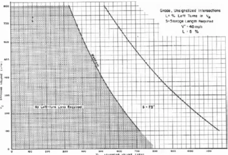
Modeling left-turn operations at unsignalized intersections has always been a challenge. The first well-known research on the operational analysis of left-turn movement was done by Harmelink. Left-turn warrants were published on the basis of queuing model with arrival and service rates assumed to be negative exponentially distributed [8]. Harmelink’s warrants stated that the probability of a through vehicle arriving behind a stopped, left-turning vehicle should not exceed 0.02 for 40 mph, 0.015 for 50 mph, and 0.01 for 60. The final criteria were presented in the form of graphs with advancing volume, opposing volume, operating speed, and left-turn percentage. One example graph of Harmelink’s criteria for determining the need for left-turn lanes is shown in Figure 1.
Figure 1 Harmelink – Left-Turn Warrant Graph 40 mph, 5% Left Turns, 1967
Most of the methods currently used to warrant left-turn lanes are based on Harmelink’s model, but the values of traffic flow parameters suggested by Harmelink should be modified [9]. A decision support system for predicting benefits of left-turn lanes at unsignalized intersections was developed based on microscopic simulation and neural networks training [10].
One of the most important measures for left-turn operations is delay. The HCM 2000 defines control delay as the measure of effectives (MOEs) for the LOS of
unsignalized intersections [1]. In this research, control delay was selected as the major MOE.
Also there’s some research work on left-turn movement treatment from safety aspect conducted in the past. In general, left-turn lanes were found to be effective in reducing total crashes at intersections. A study showed that accident reductions from
18% to 77% by adding left-turn lanes [11]. At signalized intersection, left-turn lanes were observed to reduce accident rate by 6% with permitted phasing and by 35% with protected/permitted phasing [12]. The installation of left-turn lanes was also helping to reduce left-turn crashes [13]. The researchers also found that at intersections with left-turn lanes, rear-end, sideswipe, and left-left-turn crashes were reduced compared to intersections without left-turn lanes, but right-angle crashes increased [14].Another research team found that added left-turn lanes were effective in reducing total crashes as well as fatal and injury crashes [15].
Critical Gap Calibration
Critical gap was defined as the minimum time interval in the major-street traffic stream that allows intersection entry for one minor-street vehicle [1]. The HCM 2000 gave a set of critical gap and follow-up time values as shown in Table 3, calibrated based on the U.S. conditions. 4.1 sec was the critical gap recommended for MSLT movements at both two-lane and four-lane TWSC intersections. The problem with this critical gap is that it doesn’t reflect the impacts of various factors.
Table 3 The 2000 HCM Critical Gaps and Follow-Up Times at TWSC Intersections
Vehicle Maneuver Two-Lane Major Road Critical Gap tFour Lane Major Road c Follow-Up Time tf
Left turn, major street 4.1 4.1 2.2
Right turn, minor street 6.2 6.9 3.3
Through, minor street 6.5 6.5 4.0
For estimating the critical gaps, many different models have been proposed over the past sixty years. Brilon et al. [16] gave an overview of important critical gaps calibration models, among which the models of Siegloch (1973), Raff et al. (1950), Aworth (1970), Harders (1968), Hewett (1983), and Troutbeck (1992) were the most important ones. In practice, the most commonly used models were that of Raff et al. (1950) and Troutbeck (1992). In this research, Raff’s model was employed to calibrate the critical gaps.
There are some methods summarized as logistic or logit models. The logit model was used a lot to study highway-design and safety issues. Lee and Mannering [17] employed a nested logit model to study the effect of roadside features on run-off-road accident severity. Chang and Mannering [18] used accident data to estimate a nested logit model of vehicle occupancy and accident severity. In the overview by Brilon et al. [16], the process of applying the logit model to calibrate the critical gap was introduced. Polus et al. [19] applied a disaggregate logit model to study the effect of waiting time at an approach to a roundabout on critical gaps. In this research, the logistic regression model was employed to identify the factors that affect critical gaps.
Critical gap has been found affected by some factors. For minor-street movement at unsignalized intersections, high delay was found to reduce the length of critical gap [20]. The same impact was found on roundabouts by Polus et al [19]. Driver ages were found to have some impact on the critical gaps, and the older drivers were found adopt significant longer critical gap values during nighttime [21]. The older drivers, especially older female drivers, displayed a conservative driving attitude as a compensation for
reduced driving ability [22]. In this research, factors examined included intersection geometry, posted speed limit, delay (waiting time) and some others.
Summary
Through the literature review, this research is positioned to develop a
methodology which can accurately and easily identify the impacts of platooning traffic on the operations of MSLT movement at TWSC intersections. Delay is selected as the major measure of left-turn operations at unsignalized intersection in the presence of upstream signals. The analysis of platoon scenarios at unsignalized intersections will be the main challenge in this research, since there’s no previous study on this particular topic. Raff’s critical gap model and logistic regression are selected to perform critical gap calibration for VISSIM simulation to ensure accurate results from simulation.
CHAPTER III DATA COLLECTION
The data used in this research consists of two parts. The first part is the field data collected from 30 unsignalized intersections across U.S., which is provided by the NCHRP 3-91 project. This part of data was used for critical gap calibration in this research. The second part is the simulation results from VISSIM simulation, which was used to analyze the platoon impacts on left-turn operations.
Field Data
An extensive database was established for the NCHRP 3-91 project, Left-Turn Accommodations at Unsignalized Intersections. 30 TWSC unsignalized intersections in three states of United States (Texas, Arizona, and New York) were videotaped with DV cameras, which allowed for measuring traffic volumes, gaps, gap acceptance behaviors, left-turn delay and other important information in the field. Factors related to the operations of these intersections were also recorded as part of this dataset, including intersection geometry, speed limit and signal density. Out of the field data collected from the 30 unsignalized intersections, three datasets were extracted and prepared for this research. All the 30 unsignalized intersections were listed in the table on page 18 and 19.
The information related to the gap acceptance behavior of each individual major-street left-turn (MSLT) vehicle was extracted into the gap acceptance dataset for gap acceptance behavior study. The data was recorded and prepared by each gap presented to
the driver, each row corresponding to one gap. Part of the dataset of Intersection AZ-01 is as shown in Table 4, and the elements included in Table 4 are:
Length of gaps presented to each vehicle (gaptime in Table 4),
Gap acceptance decision (response in Table 4),
Delay time in the queue (queuetime in Table 4),
Delay time at the head of queue (headtime in Table 4),
Turn time to cross approach and opposing lane (turntime1, turntime2, and
turntime in Table 4), and
Vehicle type.
Table 4 Partial Information of Gap Acceptance
Site Vehicle No. Gaptime (sec) Response Queuetime (sec) Headtime (sec) Turntime1 (sec) Turntime2 (sec) Turntime (sec) Vehicle Type
AZ-01 1 0.87 Reject 0.15 4.06 1.42 2.75 4.17 VAN
AZ-01 1 1.00 Reject 0.15 4.06 1.42 2.75 4.17 VAN
AZ-01 1 32.00 Accept 0.15 4.06 1.42 2.75 4.17 VAN
AZ-01 2 16.34 Accept 0.14 0.75 1.07 2.45 3.52 SUV
AZ-01 3 1.34 Reject 0.14 6.12 1.49 3.27 4.76 CAR
AZ-01 3 2.00 Reject 0.14 6.12 1.49 3.27 4.76 CAR
AZ-01 3 2.00 Reject 0.14 6.12 1.49 3.27 4.76 CAR
AZ-01 3 31.34 Accept 0.14 6.12 1.49 3.27 4.76 CAR
AZ-01 4 17.69 Accept 0.14 2.10 0.89 2.78 3.67 CAR
AZ-01 5 8.22 Accept 0.16 0.88 1.36 2.50 3.86 SUV
In this research, the gap acceptance data was used to perform the critical gap calibration with Raff’s critical gap model and logistic regression model. Along with the intersections characteristics in the table on page 18 and 19, the gap acceptance data
could be used to perform the detailed analysis of various factors that might affect critical gap. These factors included intersection geometry, vehicle type, speed, delay, etc.
The operational data of left-turn movement at unsingalized intersections were summarized in the second dataset for simulation calibration purpose. An example of the operational dataset is as shown in Table 5. The elements in the operational data table include:
Start time of each 5-minite period recorded,
Advancing, opposing, and left-turning volumes of each approach lane,
Average delay time within each 5-min period (queuetime and headtime in Table 5), and
Queue length.
The values of variables in Table 5 are the basis for deciding appropriate ranges for these variables in simulation scenario designing process. Besides, Table 5 contains the average MSLT delay within each 5-min period, which has been selected as the major measure of intersection operation levels. As one important step of the critical gap
calibration, the delay outputs from VISSIM simulation using Raff’s critical gap and logistic critical gap will be compared with this real-world delay to decide the better value for the critical gap of each intersection.
Table 5 Partial Information of Operation Data
Site Start Queuetime Headtime Queue Major NB/WB Vol. Major SB/EB Vol. Time (sec) (sec) Length Left Thru Right Left Thru Right
AZ-01 15:45:00 0.15 2.78 0 5 70 0 0 52 0 AZ-01 15:50:00 0.15 11.16 0 3 74 0 0 47 3 AZ-01 15:55:00 0.15 0.27 0 2 74 0 0 56 2 AZ-01 16:00:00 0.15 0.24 0 2 112 0 0 42 0 AZ-01 16:05:00 0.16 0.45 0 1 86 0 0 35 1 AZ-01 16:10:00 0.17 4.59 0 4 104 0 0 45 2 AZ-01 16:15:00 0.16 4.51 0 7 98 0 0 53 0 AZ-01 16:20:00 0.16 0.99 0 2 93 0 0 44 0 AZ-01 16:25:00 0.17 2.8 0 3 86 0 0 49 5 AZ-01 16:30:00 0.15 7.17 0 3 111 0 0 61 1
The last dataset, which summarizes the characteristics of each intersection, is partially shown in Table 6. Variables in this table include:
Number of legs,
Direction of the observed MSLT movement (Left-Turn Approach in Table 6),
Number of segment lanes and left-turn lanes (No. of LTL in Table 6),
Major Street name,
Signal density,
Number of lanes,
Posted speed limit, and
Median type and width.
The characteristics information contained in Table 6 was the basis for deciding the scenarios in simulation. The combinations of different characteristics provided in this
spreadsheet were coded in later simulation development. Besides, it was also necessary for identifying and investigating the contributing factors to the critical gap.
18
Table 6 TWSC Intersection Characteristics
Site
Num of Legs
Left-Turn
Approach Major Name
Signal Density
LTL (1=Yes,
0=No)
Median Type Median Width (ft) Num of Lanes Speed Limit (mph) AZ-01 4 Legs NB 32nd 1 1 TWLTL 10.00 2 40
AZ-02 3 Legs NB Tatum 0 1 LTL w/o Median 12.00 2 45
AZ-03 3 Legs NB Central 0 0 None 0.00 2 40
AZ-04 3 Legs EB Stanford 0 1 TWLTL 13.00 1 25
AZ-05 3 Legs NB Central 1 0 None 0.00 2 40
AZ-06 3 Legs EB Campbell 1 0 None 0.00 1 30
AZ-07 4 Legs EB CamelBack 2 0 None 0.00 1 25
AZ-08 3 Legs NB 40th Street 1 1 TWLTL 11.00 2 35
AZ-09 4 Legs NB 64th St 0 1 TWLTL 10.00 2 40
AZ-10 4 Legs EB Oak 1 0 None 0.00 1 25
AZ-11 3 Legs NB 40th Street 0 1 TWLTL 9.00 1 35
AZ-12 3 Legs EB Indian School 1 1 TWLTL 11.00 2 40
AZ-13 4 Legs EB SR 84 0 1 LTL w/o Median 0.00 2 55
AZ-14 3 Legs WB Cornville 0 1 LTL w/Flush Median 1.00 2 50
AZ-15 3 Legs EB SR 347 0 1 LTL w/Flush Median 14.00 3 55
NY-01 3 Legs WB Jefferson 1 0 None 0.00 2 30
NY-02 3 Legs NB Hyland 1 0 Raised 3.67 2 35
NY-03 4 Legs EB Forest 1 0 None 0.00 1 30
NY-04 3 Legs NB South Avenue 1 1 LTL w/Raised Median 2.67 2 40
TX-01 3 Legs SB Wellborn 0 1 TWLTL 12.00 1 45
19 Table 6 Continued Site Num of Legs Left-Turn
Approach Major Name
Signal Density
LTL (1=Yes,
0=No)
Median Type Median Width (ft) Num of Lanes Speed Limit (mph)
TX-03 3 Legs EB Spring Cypress 1 0 None 0.00 2 30
TX-04 3 Legs SB Aldine West 0 0 None 0.00 2 35
TX-05 3 Legs NB Cypresswood 0 1 LTL w/ Raised Median 32.00 2 45
TX-06 3 Legs NB Wellborn 0 0 Flush 4.17 2 45
TX-07 3 Legs WB University 0 0 None 0.00 1 60
TX-08 4 Legs WB Shadow Creek 1 1 None 0.00 1 40
TX-09 4 Legs NB Fry 0 1 LTL w/ Raised Median 14.50 2 40
TX-10 4 Legs EB Broadway 0 1 TWLTL 13.00 2 40
Simulation Results
The second part of the data used in this research was collected from the VISSIM simulation for the platoon impacts analysis. After the calibration work was finished, the VISSIM simulation was used to simulate different TWSC intersection scenarios with different types of platoons generated by upstream traffic signals. After the simulation work was finished, the left-turn delay at the downstream intersections was collected as the main measure of the operational well-being as well as some other useful data. An example of the simulation results of left-turn delay was shown in Table 7, whose elements include:
Scenario number in the simulation,
Platoon Time Ratio (see details in Chapter IV),
Platoon Flow Ratio (see details in Chapter IV),
Left-turn Delay within 1-hr period (see details in Chapter IV), and
Table 7 Simulation Results Scenario No. Platoon Time Ratio (4veh/10s) Platoon Flow Ratio (4veh/10s) Platoon Time Ratio (5veh/10s) Platoon Flow Ratio (5veh/10s) Platoon Time Ratio (6veh/10s) Platoon Flow Ratio (6veh/10s) LT Delay (s/veh) Total Delay (s/veh) Out-1-1 0.18 2.36 0.09 2.76 0.05 3.08 5.2 0.7 Out-1-2 0.19 2.35 0.13 2.65 0.06 3.11 10.1 0.7 Out-1-3 0.22 2.22 0.09 2.70 0.05 2.98 5.3 0.7 Out-1-4 0.21 2.24 0.11 2.64 0.06 3.07 7.8 0.8 Out-1-5 0.21 2.26 0.12 2.64 0.07 3.00 6.3 0.7 Out-1-6 0.18 2.33 0.09 2.75 0.04 3.17 7.7 0.7 Out-1-7 0.20 2.27 0.09 2.79 0.06 3.04 7.7 0.7 Out-1-8 0.19 2.26 0.10 2.63 0.04 3.04 5.9 0.8 Out-1-9 0.23 2.09 0.10 2.52 0.05 2.80 12.4 0.9 Out-1-0 0.18 2.46 0.12 2.81 0.07 3.24 8.1 0.9
The simulations results table includes the left-turn and total delay data at the unsignalized intersections from simulation, also the values of the two platoon
parameters. These data will be used to analyze the platoon impacts on left-turn delay and establish the relationship if the impacts do exist. Details of this analysis will be presented in Chapter IV.
CHAPTER IV METHODOLOGY
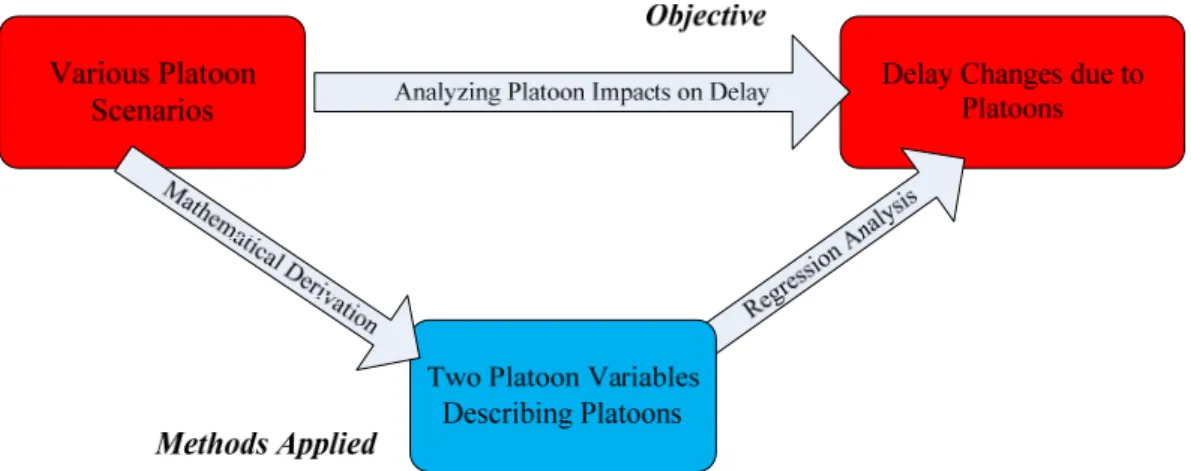
The objective of this research is to develop a methodology for analyzing and estimating the platoon effects on the MSLT delay at TWSC intersections. The main idea is to use a microscopic simulation tool to simulate different platoon scenarios in
opposing through traffic and applying regression models to capture the impacts of platoons on the delay of MSLT. The challenge in this research comes from the large number of factors affecting the platoons, which form complex combinations and make it difficult to analyze the platoon impacts. In order to solve this problem, two platoon variables were defined as a simplification of the complex platoon scenarios, making it practical to perform the analysis on platoon effects on delay. The structure of this research is illustrated in Figure 2.
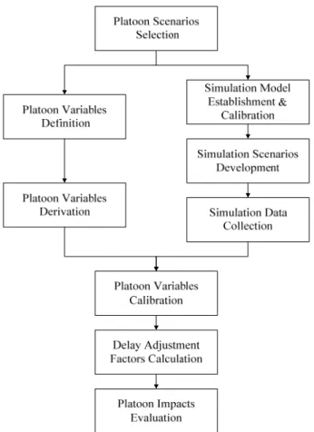
This methodology includes: simulation model establishment and calibration, simulation scenarios development, platoon parameters derivation and calibration and delay adjustment with platoon effects. The steps are shown in Figure 3.
Figure 3 Steps in Research Methodology
Simulation Model Establishment and Calibration
VISSIM, developed by PTV AG, Karlsruhe, was selected as the platform for performing the simulation work in this research [23]. VISSIM is a leading microscopic simulation program for multi-modal traffic flow modeling. It provides high-accuracy
traffic simulation through allowing users to adopt detailed input values and tune a large number of parameters in the model.
Two-way stop-control (TWSC) unsignalized intersections were coded and simulated in VISSIM to fulfill the goal of this research. The intersections simulated in this research are four-leg intersections, with two major streets and two minor streets. The MSLT movement, which is the focus of this research, is controlled by a gap acceptance model established through a function called “Priority Rule” in VISSIM. “Priority Rule” allows users to specify values for the critical gap. Minor-street movements are controlled by stop signs.
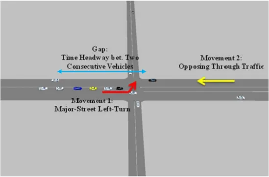
The idea of gap acceptance model of left-turn movement at unsignalized
intersection is illustrated through the example in Figure 4. In Figure 4, a group of MSLT vehicles are waiting to take a permissive left-turn at the unsignalized intersection, which is denoted by the red arrow. The left-turn vehicles have to wait for a sufficiently large gap among opposing through traffic to make a safe left-turn. The gap is also shown in Figure 4 by the blue arrow, which is defined as the time headway between two
consecutive vehicles. The gap is the most important data in the process of simulation parameter calibration. The gap data, intersection characteristics data and other related information used in this research are provided by Dr. Kay Fitzpatrick. An introduction to the datasets has been made in Chapter III.
Figure 4 Chart of Gap Acceptance Model
Two methods were employed to perform the critical gap calibration and analysis of various factors’ effects on the critical gaps: Raff’s critical gap model, and logistic regression model.
Raff’s Critical Gap Model
Raff’s method is the most commonly used method for estimating critical gaps. The definition is that critical gap value is the length of gap whose probability of being accepted equals its probability of being rejected. This method can also be interpreted as the cumulative probability where functions 1 – Fr(t)and Fa(t) intercept as shown in
1F tr( )F ta( ) (3)
where F ta( )= cumulative distribution function for the accepted gaps, ( )
r
F t = cumulative distribution function for the rejected gaps.
To calibrate the critical gap with Raff’s method in this research, the gap acceptance data collected for NCHRP 3-91 project was used. The dataset’s form was shown in Table 4, which included information of length of gaps, gap acceptance decision, delay time in the queue, delay time at the head of queue, turn time to cross approach and opposing lane. The whole dataset was divided into 30 sub-datasets by intersection, and at each individual intersection, the gaps being accepted by drivers and that being rejected were separated. The statistics programming software R was used to calculate 1 – Fr(t)and Fa(t), which are two essential variables for exploring the Raff’s
0 2 4 6 8 10 0. 0 0 .2 0. 4 0 .6 0. 8 1 .0
AZ-01 Raff’s Critical Gap
Length of Gap(sec)
P
robab
il
ty
Figure 5 AZ-01 Raff's Critical Gap
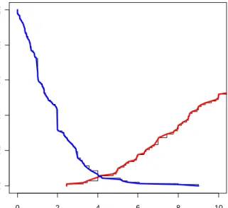
As an example, the Raff’s Critical Gap Plot is shown in Figure 5. The cumulative probability function was plotted for F ta( ) and 1F tr( ) for the intersection “Arizona-01”. The red line and the blue line denote the cumulative probability function of F ta( ) and 1F tr( ) respectively based on the gap data. The gap length of the point where two lines intersected was considered as the critical gap from this method. In this example, the critical gap for intersection “Arizona-01” was 4.1 second. The same operation was repeated for all 30 unsignalized intersections to calculate the Raff’s critical gap.
Logistic Regression Model
The second method used in this research to calibrate the critical gap is logistic regression model. Unlike regular dependent variables in linear regressions, the
dependent variable in gap acceptance model is based on a series of “accept”/ “reject” responses [24]. Ideally such responses follow a binomial distribution and the appropriate model is the logistic regression model. Logistic regression was applied to examine the factors that potentially affect drivers’ gap acceptance behaviors and also to generate a regression model for calculating the critical gap based on the field data.
The first step was to establish a gap acceptance model to calculate the probability that drivers accept a gap, taking into consideration the factors that may affect the critical gaps, including the length of gap, intersection geometry, posted speed limit, and waiting time at the head of the queue. The gap acceptance dataset shown in Table 4 was grouped into sub-datasets by intersection, and the gap acceptance probability model was
established for each individual unsignalized intersection.
For each intersection, probability of accepting a gap, the dependent variable, in a logistic regression was converted to the log of the odds ratio, as shown in Equation 4. This is known as the logit. This is the dependent variable against which independent variables are regressed.
log 1 logit (4)
1
= the ratio of probability of “accept” to that of “reject”.
Therefore, the logistic regression for calculating the probability of a particular gap being accepted can be established in the format in Equation 5. The terms of i xi are
introduced into the logit equation to account for the contributing factors that may have impacts on the gap acceptance behavior of drivers. The only contributing factor in this research is the length of gaps presented to each vehicle. Other factors including delay time in the queue, delay time at the head of queue, turn time to cross approach and opposing lane are not considered in this research because 1) length of the gap is the dominating factor that affects gap acceptance behavior, and 2) other factors cannot be reflected in the simulation. Equation 6 is the form of the model used to perform logistic regression for each intersection.
0 1 1 2 2 log ... 1 i i logit x x x (5) 0 1 log 1 gap logit x (6)
where 0 = intercept in the logistic regression model,
i
= coefficient for xi in the logistic regression model,
xi = an independent variable in the logistic regression model, and
Based on the field gap data, the parameters in Equation 6 were calibrated using maximum likelihood estimation with statistical tools. Once the logistic regression model was established based, the probability of being accepted or rejected could be calculated using Equation 7. 0 1 1 1 exp( { xgap}) (7)
The second step of calibrating the critical gap with logistic regression model was to define and calculate the critical gap for each intersection. In this research, the critical gap was defined as the gap for which the probability of accepting it according to the logistic regression model is equal to rejecting it, i.e. if 1 0.5, the gap length was considered as the critical gap. This calibration process was repeated for all the 30
intersections in the dataset.
Comparison of the Two Methods
Two sets of critical gaps were calibrated for all the 30 intersections with Raff’s model and logistic regression model respectively. Both of the two sets of critical gaps were tried in the VISSIM simulation and the delay was collected from the simulation in periods of 5 minutes for around 100 MSLT vehicles. Squared deviation between the simulated delay and the field data was calculated to compare the two sets of critical gaps and decide which one matches the real-world data better.
Table 8 Comparison of Raff’s and Logistic Method
Time Bin LT Delay (10 run average) LT Delay from Squared Deviance (vs. Field Data) (5 min) Using Raff's
Critical Gap
Using Logistic
Critical Gap Field Data
Using Raff's Critical Gap Using Logistic Critical Gap 1 2.17 3.05 2.93 0.58 0.01 2 2.06 2.05 11.32 85.75 85.93 3 4.28 4.64 0.42 14.90 17.81 4 2.22 2.46 0.39 3.35 4.28 5 0.38 0.38 0.61 0.05 0.05 6 1.53 1.65 4.76 10.43 9.67 7 2.67 3.45 4.67 4.00 1.49 8 3.12 3.56 1.15 3.88 5.81 9 4.56 4.56 2.97 2.53 2.53 10 2.72 3.66 7.32 21.16 13.40 11 4.06 4.53 1.77 5.24 7.62 12 2.72 2.99 1.18 2.37 3.28 13 4.61 5.14 0.94 13.47 17.64 14 2.81 3.03 2.57 0.06 0.21 15 2.1 2.28 4.37 5.15 4.37 16 1.57 2.44 3.81 5.02 1.88 17 2.69 2.74 3.4 0.50 0.44 18 1.6 2.19 4.16 6.55 3.88 19 1.8 1.95 5.21 11.63 10.63 20 2.61 2.79 2.34 0.07 0.20 21 3.48 3.89 7.75 18.23 14.90 22 2.5 2.66 2.75 0.06 0.01 23 2.73 3.07 24.12 457.53 443.10 24 3.34 3.86 4.35 1.02 0.24 25 2.77 3.36 4.63 3.46 1.61 26 2.4 2.76 3.5 1.21 0.55
Total of Squared Deviation 678.22 651.53
As illustrated by the example of Intersection AZ-01 in Table 8, the critical gap with smaller total squared deviation was selected as the final critical gap for this particular intersection. The Raff’s critical gap calibrated for AZ-01 is 4.1 seconds and logistic critical gap is 4.5 seconds. Both critical gaps were used to calibrate the
simulation and the left-turn delay results were collected. The deviation of left-turn delay values from VISSIM simulation vs. the field delay data were calculated in this example, which served as the measure for final decision. Critical gap that gave smaller squared deviance of left-turn delay between the simulated results and real-world data was chosen as the final critical gap. In this example, Raff’s critical gap gives a squared deviance value of 678.22 while logistic critical gap gives 651.53, which means the final critical gap for AZ-01 will be the 4.5-second logistic critical gap.
The selection of critical gap will be performed for all the 30 intersections and the final set of critical gaps will be further investigated in terms of contributing factors that may influence the critical gap at an unsignalized intersection. T-test will be applied to find out the factor that have impacts on the critical gap and a specific table of critical gaps will be recommended for the simulation of platooning scenarios.
Simulation Scenarios Development
First, four intersection categories were defined: two-lane with a left-turn lane (LTL), two-lane without a LTL, four-lane with a LTL and four-lane without a LTL.
Second, for each intersection category, a set of operational scenarios was coded, each scenario representing a certain combination of approach volume, opposing volume, the observed left-turn volume, and speed limit. When generating these scenarios,
advancing and opposing volumes were varied between 400 and 800 Vehicles per hour per lane(vphpl) at an increment of 200 vphpl and left-turn volume was varied between
20 and 140 vphpl at an increment of 40 vphpl. Speed limits included 30 mph, 40 mph, and 50 mph.
Finally, for each scenario, a fix-timed traffic signal was installed upstream from the observed unsignalized intersection to generate platoon arrivals for MSLT movement at the downstream intersection. A set of 27 upstream traffic signals were coded for each scenario to generate platoons of various intensities. The traffics signals were set up based on combinations of distance to the downstream intersection, with cycle length and green-red split as shown in Table 9.
Table 9 One Set of Upstream Traffic Signals
Distance (ft) Cycle Length (sec) Green-red Split 600 60 40/20 30/30 20/40 90 60/30 45/45 30/60 120 80/40 60/60 40/80 1500 60 40/20 30/30 20/40 90 60/30 45/45 30/60 120 80/40 60/60 40/80 2400 60 40/20 30/30 20/40 90 60/30 45/45 30/60 120 80/40 60/60 40/80
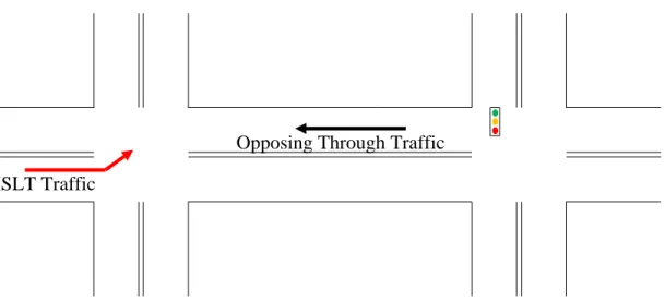
A typical Simulation Scenario of unsignalized intersection simulated in this research is shown in Figure 6. The red arrow denotes MSLT traffic and the black arrow stands for opposing through traffic coming from upstream signalized intersection.
Figure 6 Simulation Scenario Example
Each scenario’s simulation lasted for 3600 seconds and was repeated ten times with different random seeds in VISSIM, with the ten-run average as the final result. The output from all these runs formed a comprehensive dataset, among which control delay (s/veh) was used as the major performance measure of left-turn operation at each
scenario. The number of arrivals of opposing through traffic within each 10-second time interval during a 1-hour period was also recorded to calculate platoon related variables in later sections. Some other related variables were also calculated and added into the dataset if they are necessary for the platoon impacts analysis.
MSLT Traffic
Platoon Variables Definition and Calibration
A number of factors affect the platoon arrivals from an upstream signalized intersection to a downstream unsignalized intersection. These factors include hourly through traffic volume, traffic signal timing plan (cycle length and green-red split), the arrival times of through vehicles to the signalized intersection with respect to its signal state, the level of platoon dispersion occurring between the signalized intersection and the downstream unsignalized intersection. This is a fairly long list, which makes it very difficult to analyze all the combinations of these factors while identifying patterns, as well as being able to present the results in a meaningful way.
As mentioned in the literature part, for analysis of platoon effects at signalized intersection, the variable of platoon ratio (Rp) was defined to describe the platoons at
signalized intersection. In order to simplify the analysis and better present the results, similar idea was brought up for this research. Due to the complexity of platoons at unsignalized intersection, two variables (the platoon time ratio and the platoon flow ratio) were defined for describing the platoon arrivals, and they can be calculated using a platoon dispersion model.
Platoon time ratio (Rpt), is defined as the ratio of the time with platoons in
opposing through traffic to the total time within the period of one hour. Platoon flow ratio (Rpf), is defined as the ratio of average flow rate in the time with platoons to the
overall averaged flow rate within in the period of one hour. Two sets of the same variables (but from different sources) were involved in this research.
The first set of platoon variables was derived using a platoon dispersion model, and the two variables were defined as platoon time ratio from derivation (RDpt) and
platoon flow ratio from derivation (RDpf). The purpose of the first set of platoon variables
was to deal with the huge number of combinations of factors that affected platoons, which combined all the factors and describe the platoons with simply two variables.
The platoon time ratio of the first set of platoon variables (RDpt) could be derived
with a platoon dispersion model. The derivation was found in literature (Bonnesson, 1996), which can be summarized as:
,min ,max ,min ,min ,min ln[(1 )( )] ln(1 ) 0.0 o o u o u q o p o v v v f sf v v f g sf v t F sf v (8) p D pt t R C (9) with , ,max [1 (1 ) ] q g o p o o v v f F n (10) 1 1 a F t (11) ( ) u q u C g v g s v (12) a D t S (13)
1 in 0.0 c v f v
(14) whereRDpt= platoon time ratio from derivation;
f = portion of opposing stream that originated as a through movement at the upstream signalized intersection;
F = smoothing factor;
gq = effective green time required to discharge the stopped queue of the
opposing through movement at the upstream signalized intersection (sec);
vo,max = maximum flow rate in the opposing traffic (vpspl);
vo,min = user–defined minimum flow rate for platoons in the opposing traffic
(vpspl);
= platoon dispersion factor;
= ratio of travel time of lead platoon vehicle to average platoon vehicle (= 0.80);
ta = average travel time from the upstream signalized intersection to the subject
movement (sec);
tp = time with platoons within one cycle (sec);
C = cycle length of the upstream signalized intersection (sec);
g = effective green time for the opposing through movement at the upstream intersection (sec);
vu = flow rate of the opposing through movement at the upstream intersection
(vpspl);
D = distance between the upstream signalized intersection and the subject movement (m);
S = average running speed of the platoon (m/sec);
s = saturation flow rate of the conflicting through movement at the upstream signalized intersection
no = number of lanes serving the opposing through traffic;
vin = flow rate of all movements that enter the arterial and travel in the same
direction as the opposing through movement;
vo,p= flow rate of the opposing traffic during the platoon period (vps);
vo,n= flow rate of the opposing traffic during the non-platoon period (vps); and
vo= average flow rate of the opposing traffic (vps).
The platoon flow ratio of the first set (RDpf) was derived and summarized in this
research in Equation 15 and 16. Detailed derivation process was documented in Appendix A.
,min ,max , 1 1 1 (1 ) ( ) ( ) ln(1 ) q g o o a p q b u e q F v v sf n sf g t v f t g F (15) , a p D pf o p n R v t (16) with ,min ln(1 ) ln(1 ) o b v sf t F (17) ,min ,max ln( ) ln(1 ) o u o u e q v v f v v f t g F (18) whereRDpf = platoon flow ratio;
na,p = number of arrivals in platoon intervals;
tb = the beginning time of the platoon; and
te = the ending time of the platoon.
The second set was calculated from the platoon arrival data collected from the simulation, and the two variables were defined as platoon time ratio from simulation (RSpt) and platoon flow ratio from simulation (RSpf). The second set of platoon variables
was used directly in the analysis of platoon impacts on delay, and was also used as the yardstick to calibrate the derivation equations for the first set of platoon variables. As mentioned earlier, the number of arrivals of opposing through traffic within each 10-second time interval during a 1-hour period was recorded for this calculation. In this research, the intervals with more than 3 arrivals (3vehicles/10seconds) at two-lane
intersections were defined as the platoon intervals, while 5 arrivals (5vehicles/10seconds) was the critical value for four-lane intersections.
The two platoon variables of the second set (RSpt and RSpf), can be calculated
based on the data collected from simulation using the following equations:
, , , 10sec 10sec 3600sec 360 10sec i p i p i p S pt i R n n n n (19) , , , 3600sec / / 10sec a p a p S a pf o p o S i p a pt n n n R v v n n R , (20) where
RSpt = platoon time ratio from simulation;
RSpf = platoon flow ratio from simulation;
ni,p = number of platoon intervals ;
ni = number of all intervals within 1 hour;
na,p = number of arrivals in platoon intervals; and
na = number of all arrivals within 1 hour.
Both sets of platoon variables are involved in this research to analyze the platoon impacts on MSLT delay. The purpose of the first set of platoon variables (RDpt and RDpf
) is to combine all the factors that affected platoons and describe the platoons in a simple way. The second set of platoon variables (RSpt and RSpf) is used directly for the analysis
of platoon impacts on delay and for the calibration of the first set.
However, the mathematical derivations do not necessarily match the simulation results perfectly, since the VISSIM simulation tool does not adopt the same platoon dispersion model with which the mathematical derivation is performed. Even during a period of platoon arrival, the headway between vehicles and arrival flow rate may
fluctuate in the real-world and in micro simulation. A practical method that combines the two sets of platoon variables was proposed in this research, one that could both handle the large number of combinations of related factors, and serve as the basis for platoon impacts on MSLT delay.
Therefore, further calibration of the derivation equation with the data collected in the simulation is needed before use. A linear regression model was developed to identify the relationship between the variable values from derivation and those from simulation. This calibrated regression model can then be used for further platoon impacts analysis from given scenarios.
Delay Adjustment with Platoon Effects
After using the two platoon variables to describe platoon arrivals, the next step is to look into how the platoon arrivals in opposing through traffic affect the delay of MSLT movement at TWSC intersections. In order to quantify the platoon arrivals’ impacts, the delay adjustment factor (Fda) was defined. Fda was defined as the ratio of
left-turn delay under platoon arrivals in opposing through traffic to that under random arrivals. The Fda is a measure of how much the platoon arrivals are changing the left-turn
delay from random-arriving situations. In this research, Fda was calculated for each
1-hour/3600-sec period based on the delay data collected from the simulation.
p da r d F d (21)
where
dp = MSLT delay under platooning arrivals in each 3600-sec scenario, and
dr = MSLT delay under random arrivals in each 3600-sec scenario.
If some relationship between the two platoon variables (RSptand RSpf) and the
delay adjustment factors (Fda) can be found, the impacts of platoon arrivals in opposing
through traffic will be evident. Linear or other forms of regression models could be employed to establish the relationship between the two platoon variables and Fda.
CHAPTER V RESULTS
Critical Gap Calibration Results
Raff’s critical gap model and logistic regression model were adopted in this research to calibrate the critical gaps of the 30 intersections involved in the dataset. As mentioned in Chapter IV, the calibration was performed by each individual intersection.
For the Raff’s model, the curves of a particular gap being accepted and rejected were plotted on the same chart and the intercepting point of the two curves is the critical gap for the intersection. One example is shown in Figure 5 and the complete collection is in Appendix B.
For the logistic regression model, the gap value making the probability of the gap equal to 0.5 is defined as the critical gap. The probability model was established in the form of logistic regression, setting driver response as the dependent variable and length of the gap as the independent variable. The collection of results is shown in Appendix C.
The two sets of critical gaps from Raff’s critical gap model and logistic
regression model were tested in the VSSIM simulation in order to decide which critical gap of the two yielded simulation closer to the field data. The critical gap with smaller squared deviation of delay from the field delay data was chosen as the final critical gap for each intersection. The Raff’s critical gaps, logistic regression critical gaps and the squared deviation of delay between real-data delay and simulation delay using respective critical gap were summarized in Table 10. The critical gap that led to a better fit of the
real-world was chosen as the final critical gap for each intersection. See detailed process in Table 8 and the whole collection in Table 10.
Also observed from the comparison of the two models was that Raff’s model and logistic model calibration did not show significant difference in total squared deviation of left-turn delay. Through this comparison, Raff’s model was actually preferred, because logistic regression was much more sophisticated model but giving similar results, which should be avoided when choosing the calibration model. Therefore, for future calibration work, Raff’s model was recommended unless other complicated model could yield results of significantly better quality.
Table 10 Critical Gaps from Raff's and Logistic Regression Model Site Raff’s Critical Gap Squared Deviation of Delay Logistic Critical Gap Squared Deviation of Delay Final Critical Gaps AZ-01 4.1 678.217 4.5 651.534 4.5 AZ-02 3.4 88.9696 2.2 112.041 3.4 AZ-03 3.9 329.010 3.6 340.171 3.9 AZ-04 6.6 364.812 6.2 385.405 6.6 AZ-05 4.0 1416.17 4.5 1364.870 4.5 AZ-06 4.4 333.203 4.4 333.203 4.4 AZ-07 6.4 116.499 5.4 107.503 5.4 AZ-08 4.5 174.134 4.6 163.675 4.6 AZ-09 4.9 594.788 4.9 594.788 4.9 AZ-10 4.9 26.272 1.8 17.376 4.9 AZ-11 4.8 1982.000 5.4 1892.710 5.4 AZ-12 4.1 1134.570 5.6 1216.270 4.1 AZ-13 7.8 466.196 6.2 471.715 7.8 AZ-14 4.7 -- 4.9 -- 4.8 AZ-15 5.2 42.522 4.9 43.105 5.2 NY-01 3.9 742.247 3.8 718.533 3.8 NY-02 3.3 1744.750 4.5 1243.390 4.5 NY-03 4.0 397.900 4.3 397.739 4.3 NY-04 4.9 -- 5.6 -- 5.25 TX-01 4.6 898.590 4.8 838.333 4.8 TX-02 6.0 24.590 5.0 42.601 6 TX-03 4.2 744.586 5.2 423.022 5.2 TX-04 3.9 148.921 3.3 162.899 3.9 TX-05 6.0 330.947 4.7 487.201 6 TX-06 5.3 127.124 4.9 147.801 5.3 TX-07 5.8 426.190 5.7 430.127 5.8 TX-08 4.4 583.957 4.7 541.430 4.7 TX-09 4.2 3071.590 5.6 3214.590 4.2 TX-10 3.1 1026.030 4.7 838.392 4.7 TX-11 4.5 179.974 4.8 152.603 4.8
Based on the final critical gaps established in Table 10, a further analysis on critical gaps in terms of the geometric and operational characteristics of the intersection was performed to get more accurate critical gap for simulation. The final critical gaps and intersection factors were summarized in Table 11. The factors that potentially affect the critical gap values were chosen from Table 6 for the analysis. The factors included:
Number of legs (No. of Legs in Table 11),
Number of lanes (No. of Lanes in Table 11),
Median presence,
Posted speed limits, and
Average waiting time at the head of the queue for left-turn at each intersection (Avg. Waiting Time in Table 11).
Table 11 Final Critical Gap Values for Each Intersection
Site Final Gaps (sec) No. of Legs No. of LTL No. Lanes Median Presence Median Width (ft) Speed Limit (mph) Avg Waiting Time (sec) AZ-01 4.5 4 1 2 1 10 40 3.66 AZ-02 3.4 3 1 2 1 12 45 1.95 AZ-03 3.9 3 0 2 0 0 40 2.75 AZ-04 6.6 3 1 1 1 13 25 3.45 AZ-05 4.5 3 0 2 0 0 40 4.94 AZ-06 4.4 3 0 1 0 0 30 1.61 AZ-07 5.4 4 0 1 0 0 25 1.1 AZ-08 4.6 3 1 2 1 11 35 3.36 AZ-09 4.9 4 1 2 1 10 40 3.68 AZ-10 4.9 4 0 1 0 0 25 0.6 AZ-11 5.4 3 1 1 1 9 35 5.02 AZ-12 4.1 3 1 2 1 11 40 8.27 AZ-13 7.8 4 1 2 0 0 55 1.66 AZ-14 4.8 3 1 2 1 1 50 4.08 AZ-15 5.2 3 1 2 1 14 55 2.7 NY-01 3.8 3 0 2 0 0 30 4.42 NY-02 4.5 3 0 2 1 4 35 7.67 NY-03 4.3 4 0 1 0 0 30 4.96 NY-04 5.25 3 1 2 1 3 40 6.81 TX-01 4.8 3 1 1 1 12 45 5.2 TX-02 6 4 0 1 0 0 65 1.49 TX-03 5.2 3 0 2 0 0 30 5.92 TX-04 3.9 3 0 2 0 0 35 1.64 TX-05 6 3 1 2 1 32 45 3.31 TX-06 5.3 3 0 2 1 4 45 3.44 TX-07 5.8 3 0 1 0 0 60 2.44 TX-08 4.7 4 1 1 0 0 40 2.8 TX-09 4.2 4 1 2 1 15 40 8.23 TX-10 4.7 4 1 2 1 13 40 6.92 TX-11 4.8 3 1 2 1 15 55 3.72
The overall averaged critical gap for left-turn movement at TWSC intersections is 4.9 second, calculated by averaging all the critical gaps of 30 intersections. This critical gap is larger than the 4.1 sec critical gap for left-turn movement that recommended in the 2000 HCM. It is probably due to the low traffic volume at unsignalized intersections in this NCHRP project, which needs further exploration to confirm it. Furthermore, in order to identify the factors that have impacts on critical gaps of left-turn movement, t-test was employed to compare the different critical gaps
between groups divided by potential factors. The t-test results were summarized in Table 12.
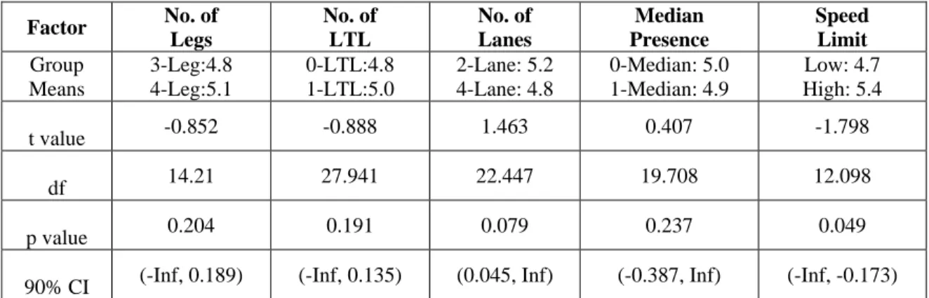
Table 12 T Test for Factors Related to Critical Gaps
Factor No. of Legs No. of LTL No. of Lanes Median Presence Speed Limit Group Means 3-Leg:4.8 4-Leg:5.1 0-LTL:4.8 1-LTL:5.0 2-Lane: 5.2 4-Lane: 4.8 0-Median: 5.0 1-Median: 4.9 Low: 4.7 High: 5.4 t value -0.852 -0.888 1.463 0.407 -1.798 df 14.21 27.941 22.447 19.708 12.098 p value 0.204 0.191 0.079 0.237 0.049
90% CI (-Inf, 0.189) (-Inf, 0.135) (0.045, Inf) (-0.387, Inf) (-Inf, -0.173)
*Note: For Speed Limit, “Low” means lower or equal to 40 mph, while “High” is higher than 40 mph.
From Table 12, two factors were found to have impacts on critical gap values. Speed limit and number of lanes were found to cause significant differences between critical gaps of different groups with 90% confidence. The impacts on critical gap values by the two factors were summarized as below:
The critical gap of two-lane intersections is significantly larger than that of four-lane intersections with 90% confidence.
Intersections with higher posted speed limit tend to have larger critical gaps than those with lower speed limit.
Therefore, critical gaps were proposed in terms of number of lanes and posted speed limit of the intersections. The updated categorical critical gap values were shown in Table 13. There are two reasons might lead to the fact that two-lane intersection has larger critical gap than that of four-lane: first, two-lane roads typically have much lower traffic volume, therefore left-turn drivers are able to take generally larger gaps; second, for a left-turn drivers, four-lane roads have two opposing lanes which decreases the chances of having large gaps, lowing drivers’ expectation and making them more
aggressive in gap acceptance. When it comes to speed limits, the higher the speed is, the higher risk there is, therefore larger critical gap has been adopted in high speed
intersection due to the safety concern.
Table 13 Recommended Critical Gap Values
Number of Lanes Final Critical Gap(sec)
Low Speed High Speed
2 5.1 5.5