Thorsten Schmidt-Dumont
Dissertation presented for the degree of Doctor of Philosophy
in the Faculty of Engineering at Stellenbosch University
Promoter: Prof JH van Vuuren
Declaration
By submitting this dissertation electronically, I declare that the entirety of the work contained therein is my own, original work, that I am the sole author thereof (save to the extent explicitly otherwise stated), that reproduction and publication thereof by Stellenbosch University will not infringe any third party rights and that I have not previously in its entirety or in part submitted it for obtaining any qualification.
Date: December2018
Copyright c2018 Stellenbosch University All rights reserved
Abstract
Traffic congestion has become a significant problem around the world, not only in first-world countries, but also in third-world countries such as South Africa. Due to spatial limitations, especially in well-developed metropolitan areas, which typically experience the worst congestion problems, capacity expansion is not always feasible for relieving the pressure on the trans-portation network. Furthermore, the theory of induced traffic demand suggests that increasing highway capacity is not a long-term solution to traffic congestion due to additional traffic de-mand on new or updated routes, induced by commuters’ perception that new or upgraded routes should be congestion free. As a result, various approaches toward improving highway traffic flow without increasing infrastructure capacity have been proposed in the literature.
Ramp metering and variable speed limits are the best-known control measures for effective traffic flow on highways. In most approaches towards solving the control problems presented by these control measures, optimal control techniques or online feedback control have been employed. Feedback control does not, however, guarantee optimality with respect to the on-ramp metering rate or the speed limit chosen, while optimal control techniques are limited to small networks due to their large computational burden.
Reinforcement learning is a promising alternative, providing the means and framework required to achieve near-optimal control policies at a fraction of the computational burden associated with optimal control algorithms. In this dissertation, a decentralised reinforcement learning approach is adopted towards simultaneously solving both the ramp metering and variable speed limit control problems.
The dawn of the autononomous vehicle promises further improvements in traffic flow which may be achieved over and above those of the aforementioned established highway traffic control measures, if their capabilities are harnessed effectively. A novel method of ramp metering by autonomous vehicles is introduced in this dissertation, based on the premise that specific instructions may be provided to autonomus vehicles travelling along an on-ramp. The control problem presented by this method of ramp meteringviaautonomous vehicles is also solved using a reinforcement learning approach.
The above solution approaches are implemented as a concept demonstrator within a simple, benchmark microscopic highway traffic simulation model. The effectiveness of the decentralised reinforcement learning approach is evaluated by means of statistical comparisons within the context of this simple benchmark simulation model. These approaches are finally applied within the context of a real-world case study simulation model of a section of the N1 highway outbound out of Cape Town, South Africa in order to demonstrate the effectiveness of the approaches within the context of a realistic scenario based on a real highway network and real traffic flow data.
Uittreksel
Verkeersopeenhoping het ’n ernstige probleem regoor die wˆereld geword, nie net in eerste-wˆereld lande nie, maar ook in derde-wˆereld lande soos Suid-Afrika. As gevolg van ruimte-beperkings, veral in ontwikkelde, stedelike gebiede wat tipies die ernstigste verkeersopeenhoping ervaar, is die uitbreiding van infrastruktuur nie altyd ’n moontlike oplossing vir druk wat op vervoer-netwerke ervaar word nie. Verder volg dit uit die teorie van ge¨ınduseerde verkeersdruk dat die verhoging van snelwegkapasiteit nie ’n langtermynoplossing vir verkeersopeenhoping is nie vanwe¨e die addisionele verkeer op nuwe of opgegradeerde roetes wat spruit uit die pendelaars-persepsie dat sulke roetes opeenhoping-vry behoort te wees. Gevolglik is ’n aantal benade-rings in die literatuur voorgestel waarvolgens snelwegverkeersvloei verbeter kan word sonder om infrastruktuurkapasiteit te verhoog.
Opritmeting en veranderlike spoedbeperkings is die mees bekende beheermaatre¨els vir doel-treffende verkeersvloei op snelwe¨e. In die meeste benaderings tot die oplossing van die beheer-probleme wat met hierdie maatre¨els gepaard gaan, word optimale beheertegnieke of intydse terugvoerbeheer toegepas. Daar is egter geen waarborg dat terugvoerbeheertegnieke optimale oplossings in terme van opritmetingstempo’s of geselekteerde spoedgrense sal lewer nie, ter-wyl die gebruik van optimale beheertegnieke beperk is tot klein vervoernetwerke vanwe¨e die noemenswaardige berekeningsvereistes van hierdie tegnieke.
Versterkingsleer is ’n belowende alternatief wat die middele en raamwerk verskaf waarvolgens byna-optimale beheerbeleide teen ’n fraksie van die berekeningsvereistes van konvensionele opti-male beheeralgoritmes geformuleer kan word. ’n Gedesentraliseerde benadering tot versterkings-leer word in hierdie proefskrif gevolg om die verkeersvloei-beheerprobleme wat met opritmeting en veranderlike spoedbeperkings gepaard gaan, gelyktydig op te los.
Die koms van die outonome voertuig beloof verdere verbeterings in verkeersvloei wat behaal kan word bo en behalwe di´e van die bogenoemde gevestigde snelwegverkeersbeheermaatre¨els, indien hul doeltreffend aangewend word. ’n Nuwe metode van opritmeting deur middel van outonome voertuie word in hierdie proefskrif voorgestel, gebaseer op die veronderstelling dat spesifieke instruksies aan outonome voertuie op ’n oprit voorsien kan word. Die beheerprobleem wat deur hierdie metode van opritmeting deur middel van outonome voertuie daargestel word, word ook met behulp van ’n versterkingsleerbenadering opgelos.
Die bogenoemde oplossingsbenaderings word as ’n konsepdemonstrator in die konteks van ’n eenvoudige mikroskopiese snelweg-toetssimulasiemodel ge¨ımplementeer. Die doeltreffendheid van die gedesentraliseerde versterkingsleerbenadering word deur middel van statistiese verge-lykings in die konteks van die bogenoemde model evalueer. Die leerbenadering word laastens ook op ’n simulasiemodel van ’n realistiese gevallestudie oor die N1 snelweg uit Kaapstad, Suid-Afrika toegepas om die doeltreffendheid daarvan in terme van ’n werklike scenario en werklike verkeersvloeidata te demonstreer.
Acknowledgements
The author wishes to acknowledge the following people and institutions for their various contributions towards the completion of this work:
• My promoter, Prof JH van Vuuren, for sharing his broad knowledge, for his patience, guidance, relentless effort and his belief in me, for his critique, the challenging questions and the continual support, all of which have contributed to the quality of the work in this dissertation, which hopefully does not disappoint, knowing that you are “easily pleased with the very best.”
• My co-promoter, Mrs Megan Bruwer from the Stellenbosch Smart Mobility Laboratory within the Department of Civil Engineering, for her assistance with regard to the traffic-specific questions, the brainstorming for ideas with respect to the novel highway traffic control measure, and her help in obtaining the traffic data required for the case study. • SUnORE, the Harry Crossley foundation and the Department of Industrial Engineering,
for their generous financial support over the past three years.
• SUnORE and the Department of Industrial Engineering, for the privilege to use the office space and computational facilities, and for affording me the opportunity to be a part of such an inspirational research environment.
• My colleagues at SUnORE, for their friendship, banter and inspiration over the past three years, making it a truly unforgettable time.
• My parents Hans and Henricke, and my brothers Georg and Andr´e, for their unconditional support whenever I needed it, throughout the course of my studies from BEng through to PhD. No matter what I had planned, you believed in me and encouraged me at every step along the way.
• Last but by no means least, my girlfriend Hester, thank you all for the unwavering support, the never-ending encouragement, for being my soundboard for ideas and allowing me to vent my frustration whenever necessary. Thank you for joining me for late nights and weekends at the office, for unexpectedly bringing me dinner when I was working late, and for always being there for me when I needed your support.
Table of Contents
Abstract iii
Uittreksel v
Acknowledgements vii
List of Reserved Symbols xi
List of Acronyms xiii
List of Figures xv
List of Tables xvii
List of Algorithms xix
1 Introduction 1
1.1 Dissertation Background and Origin . . . 1
1.2 Problem Statement . . . 6 1.3 Dissertation Objectives . . . 6 1.4 Dissertation Scope . . . 8 1.5 Research Methodology . . . 9 1.6 Dissertation Organisation . . . 10 I Literature Review 13 2 Machine Learning 15 2.1 Machine Learning in General . . . 15
2.2 Reinforcement Learning . . . 16
2.2.1 Evaluative Feedback . . . 17
2.2.2 The Reinforcement Learning Problem . . . 19
2.2.3 Reinforcement Learning Solution Approaches . . . 24
2.3 Reinforcement Learning with Function Approximation . . . 28
2.3.1 k-Nearest Neighbours Weighted Average . . . 29
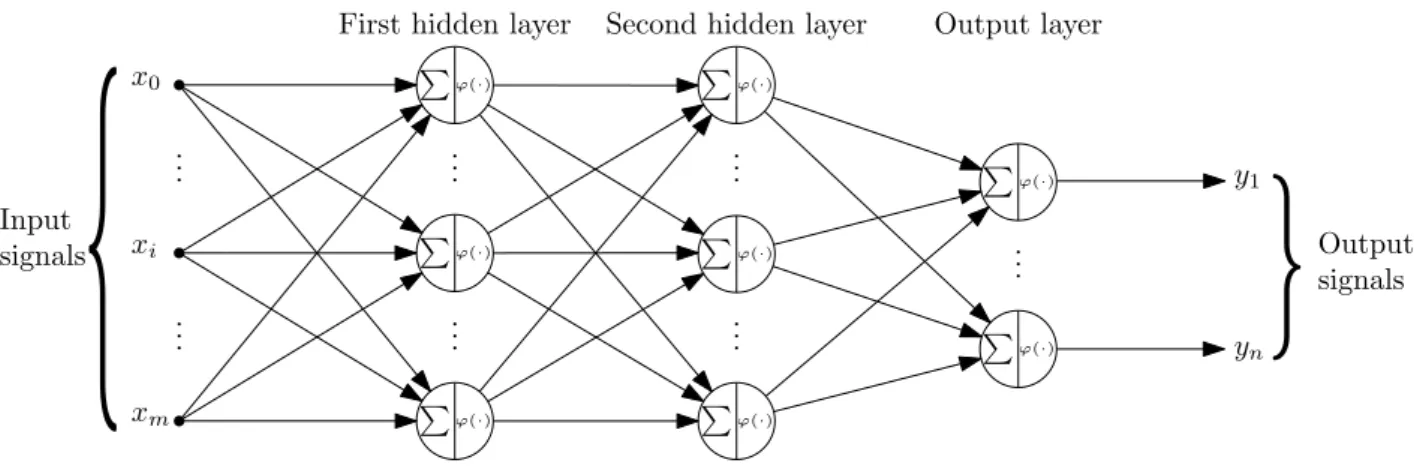
2.3.2 Multi-layer Perceptron Neural Networks . . . 30
2.4 Chapter Summary . . . 36
3 Highway Traffic Control 37 3.1 Traffic Flow Fundamentals . . . 37
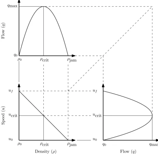
3.1.1 Macroscopic Traffic Flow Theory . . . 38
3.1.2 Microscopic Traffic Flow Theory . . . 41
3.2 Highway Traffic Control Measures . . . 44
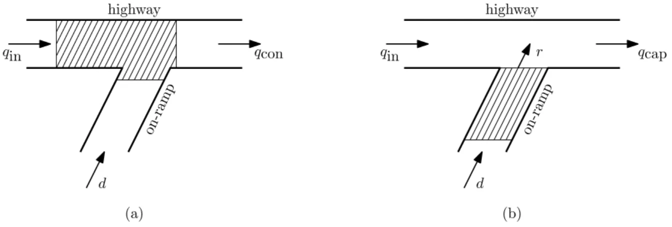
3.2.1 Ramp Metering . . . 44
3.2.2 Variable Speed Limits . . . 51
3.2.3 Lane Assignment . . . 56
3.3 Highway Control in the Presence of Autonomous Vehicles . . . 58
3.4 Machine Learning in Highway Traffic Control . . . 63
3.4.1 Reinforcement Learning for Ramp Metering . . . 63
3.4.2 Reinforcement Learning for Variable Speed Limits . . . 65
3.5 Chapter Summary . . . 67
4 Computer Simulation Modelling 69 4.1 Simulation Modelling Concepts . . . 69
4.2 Prevailing Simulation Modelling Paradigms . . . 71
4.2.1 Agent-based Modelling . . . 71
4.2.2 Discrete-event Modelling . . . 71
4.2.3 System Dynamics Modelling . . . 71
4.2.4 Dynamic Systems Modelling . . . 72
4.3 Typical Steps in a Simulation Study . . . 72
4.4 Verification and Validation of a Simulation Model . . . 75
4.4.1 Verification of a Simulation Model . . . 75
4.4.2 Validation of a Simulation Model . . . 76
4.5 Some Advantages and Drawbacks of Simulation Modelling . . . 77
4.6 Traffic Simulation Modelling Paradigms . . . 78
4.6.1 Macroscopic Traffic Simulation . . . 79
5 A Microscopic Highway Simulation Model 85
5.1 Model Framework . . . 85
5.1.1 Constructing the Road Network . . . 86
5.1.2 The Benchmark Model . . . 88
5.1.3 The Generation of Vehicles . . . 89
5.1.4 Model Output Data . . . 90
5.2 Model Verification and Validation . . . 90
5.2.1 Verification of the Traffic Simulation Model . . . 91
5.2.2 Validation of the Traffic Simulation Model . . . 91
5.3 Experimental Design . . . 93
5.3.1 The Simulation Warm-up Period . . . 93
5.3.2 General Specifications of the Simulation Framework . . . 94
5.3.3 Types of Statistical Analysis to be Performed on Model Output Data . . 96
5.4 Chapter Summary . . . 99
6 Reinforcement Learning for Ramp Metering 101 6.1 ALINEA and PI-ALINEA in a Microscopic Context . . . 102
6.2 Formulation as a Reinforcement Learning Problem . . . 102
6.2.1 The State Space . . . 102
6.2.2 The Action Space . . . 103
6.2.3 The Reward Function . . . 104
6.2.4 Learning Rate and Action Selection . . . 104
6.3 Q-Learning for Ramp Metering . . . 105
6.4 kNN-TD Learning for Ramp Metering . . . 106
6.5 Computational Results . . . 106
6.5.1 Parameter Evaluation . . . 107
6.5.2 Algorithmic Comparison . . . 110
6.6 Ramp Metering with a Queueing Consideration . . . 130
6.6.1 ALINEA and PI-ALINEA with Queue Limits . . . 130
6.6.2 Q-Learning andkNN-TD with Queue Limits . . . 131
6.7 Chapter Summary . . . 152
7 Reinforcement Learning for Variable Speed Limits 153 7.1 The Feedback-based VSL Controller Implementation . . . 153
7.2 Formulation as a Reinforcement Learning Problem . . . 154
7.2.1 The State Space . . . 154
7.2.2 The Action Space . . . 155
7.2.3 The Reward Function . . . 156
7.3 Q-Learning for Variable Speed Limits . . . 156
7.4 kNN-TD Learning for Variable Speed Limits . . . 157
7.5 Computational Results . . . 157
7.5.1 Parameter Evaluation . . . 157
7.5.2 Algorithmic Comparison . . . 159
7.6 Chapter Summary . . . 175
8 Multi-Agent Reinforcement Learning 177 8.1 An Integrated RM and VSL Feedback Controller . . . 177
8.2 An Introduction to Multi-Agent Reinforcement Learning . . . 178
8.2.1 Independent Learners . . . 178
8.2.2 Cooperative Reinforcement Learning . . . 179
8.3 MARL for Highway Traffic Control . . . 180
8.3.1 Independent MARL for RM and VSL . . . 181
8.3.2 Hierarchical MARL for RM and VSL . . . 181
8.3.3 Maximax MARL for RM and VSL . . . 183
8.4 Computational Results . . . 185
8.4.1 Reward Function Evaluation . . . 185
8.4.2 Algorithmic Comparison . . . 187
8.5 MARL with a Queueing Consideration . . . 206
8.5.1 Reward Function Evaluation . . . 206
8.5.2 Algorithmic Comparison . . . 207
8.6 Chapter Summary . . . 227
9 The N1: The Simulation Model 229 9.1 Model Description . . . 229
9.2 Input Data . . . 231
9.6 Chapter Summary . . . 240
10 The N1: Computational Results 241 10.1 Ramp Metering . . . 242
10.1.1 Algorithmic Implementations . . . 242
10.1.2 Parameter Evaluations . . . 243
10.1.3 Algorithmic Comparison . . . 250
10.1.4 Discussion . . . 257
10.2 Ramp Metering with Queue Limits . . . 259
10.2.1 Algorithmic Implementations . . . 259
10.2.2 Algorithmic Comparison . . . 260
10.2.3 Discussion . . . 266
10.3 Variable Speed Limits . . . 268
10.3.1 Algorithmic Implementations . . . 268
10.3.2 Parameter Evaluations . . . 270
10.3.3 Algorithmic Comparison . . . 273
10.3.4 Discussion . . . 280
10.4 Multi-Agent Reinforcement Learning . . . 280
10.4.1 Algorithmic Implementations . . . 281
10.4.2 Reward Function Evaluations . . . 281
10.4.3 Algorithmic Comparison . . . 282
10.4.4 Discussion . . . 287
10.5 Multi-Agent Reinforcement Learning with Queue Limits . . . 291
10.5.1 Algorithmic Implementations . . . 291
10.5.2 Algorithmic Comparison . . . 292
10.5.3 Discussion . . . 298
10.6 Chapter Summary . . . 301
III Future Technologies 303 11 Ramp Metering by Autonomous Vehicles 305 11.1 Autonomous Vehicles for Ramp Metering . . . 306
11.2 Formulation as a Reinforcement Learning Problem . . . 307
11.2.1 The State Space . . . 307
11.2.2 The Action Space . . . 308
11.2.3 The Reward Function . . . 308
11.3 Q-Learning for Ramp Metering by AVs . . . 308
11.4 kNN-TD learning for Ramp Metering by AVs . . . 309
11.5 Parameter Evaluation . . . 309
11.5.1 Target Density Parameter Evaluation . . . 310
11.5.2 On-ramp Length Parameter Evaluation . . . 313
11.5.3 AV Percentage Parameter Evaluation . . . 316
11.5.4 Traffic Demand Parameter Evaluation . . . 335
11.6 Algorithmic Comparison . . . 346 11.6.1 Scenario 1 . . . 347 11.6.2 Scenario 2 . . . 355 11.6.3 Scenario 3 . . . 357 11.6.4 Scenario 4 . . . 364 11.6.5 Discussion . . . 368 11.7 Chapter Summary . . . 369
12 Ramp Metering by Autonomous Vehicles on the N1 371 12.1 Algorithmic Implementations . . . 371
12.2 Parameter Evaluations . . . 373
12.2.1 Target Density Parameter Evaluations . . . 373
12.2.2 AV Percentage Parameter Evaluations . . . 377
12.3 Algorithmic Comparison . . . 386
12.4 Discussion . . . 395
12.5 Chapter Summary . . . 398
IV Conclusion 399 13 Summary and Conclusions 401 13.1 Dissertation Contents . . . 401
13.2 Appraisal of Dissertation Contributions . . . 406
14 Suggestions for Future Work 409 14.1 Scope Enlargement Suggestions . . . 409
List of Reserved Symbols
VariablesSymbol Meaning
at The action chosen at time stept
α The step-size parameter (learning rate)
The probability of choosing a random action during action selection γ The discount rate for future rewards
Pa
ss0 The probability of transition from state sto states0 under action a q The flow of vehicles along a section of highway
Q(s, a) The value of taking actionain state s
Q(x, a) The value associated with centre-action pair (x, a) in kNN-TD learning rt The reward obtained at time stept
Rt The return following time step t
Ra
ss0 The expected immediate reward on transition fromstos0 under actiona ρ The density on a stretch of highway
ˆ
ρ The target density that a ramp metering agent aims to achieve directly down-stream of an on-ramp
st The state of the environment at time step t
Vπ(s) The value of state sunder policy π
w The length of the queue building up at an on-ramp Sets
Symbol Meaning
A(s) The set of all possible actions in state s S The set of all nonterminal states
S+ The set of all terminal states
R The set of all rewards
List of Acronyms
AHS: Automated highway systemALINEA: Asservissement Lin´eaire d’Entre´e Autorouti`ere ANN: Artificial neural network
ANOVA: Analysis of variance AV: Autonomous vehicle AI: Artificial intelligence
CCTV: Closed circuit television CI: Confidence interval
CRM: Conventional ramp metering
CRM-QL: Conventional ramp metering with queue limits CSV: Comma separated value
CTM: Cellular transition model GIS: Geographic information system GPS: Global positioning system GUI: Graphical user interface HMI: Human machine interface IRC: Iterative run controller LA: Lane assignment
LSD: Least significant difference
kNN-TD: knearest neighbour temporal difference reinforcement learning algorithm MARL: Multi-agent reinforcement learning
MARLIN-ATCS: Multi-agent reinforcement learning for an integrated network of adaptive traffic signal controllers
MDP: Markov decision process
MLP: Multi-layer perceptron MPC: Model predictive control OSM: Open street map
PMI: Performance measure indicator RL: Reinforcement learning
RM: Ramp metering
RMART: R-Markov average reward technique
SANRAL: South African National Roads Agency Limited SARSA: State-action-reward-state-action
SATURN: Simulation and Assignment of Traffic in Urban Road Networks SUMO: Simulation of Urban Mobility
TIS: Time spent in the system by individual vehicles TMC: Traffic management centre
TTS: Total time spent in the system VMS: Variable message sign
List of Figures
1.1 Severe traffic congestion around the world . . . 2 1.2 Congestion levels in Cape Town and Johannesburg during 2009–2016 . . . 3 1.3 Sensor configuration on an autonomous vehicle . . . 4 1.4 Expected autonomous vehicle adoption rates . . . 5
2.1 The agent-environment interaction in reinforcement learning . . . 19 2.2 Backup diagrams for a specific state sand a specific state-action pair (s, a) . . 20 2.3 Illustration of thek-nearest neighbour algorithm . . . 29 2.4 The nonlinear model of a neuron . . . 32 2.5 The logistic sigmoid activation function . . . 32 2.6 The single-layer perceptron model . . . 33 2.7 Linear separability of two surfaces . . . 33 2.8 The multi-layer perceptron model . . . 34
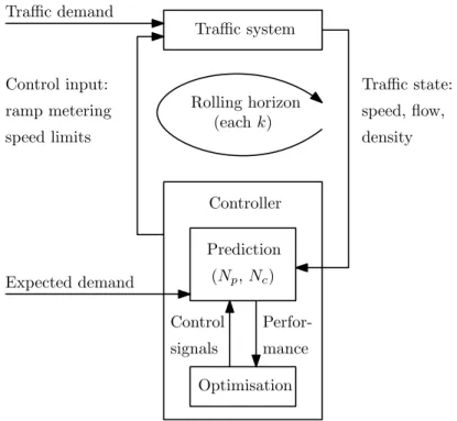
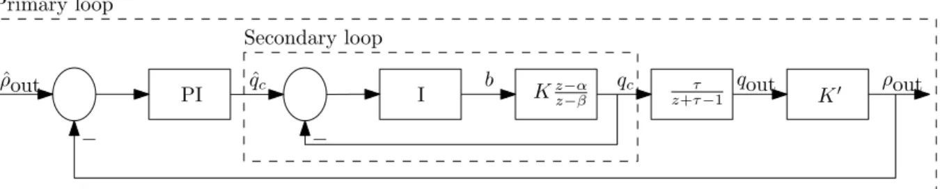
3.1 The fundamental diagrams of traffic flow . . . 40 3.2 A time-space diagram illustrating time and space headways . . . 42 3.3 Car-following theory notations and definitions . . . 43 3.4 A ramp metering comparison . . . 45 3.5 Functional structure of the demand-capacity and ALINEA algorithms . . . 47 3.6 A schematic illustration of an MPC structure . . . 50 3.7 A hierarchical MPC control structure . . . 51 3.8 The effect of VSLs on the fundamental diagram of traffic flow theory . . . 52 3.9 An MTFC feedback cascade controller . . . 55 3.10 Velocity profile of a vehicle creating a space for lane changing . . . 57 3.11 An adaptive cruise control controller architecture . . . 59 3.12 Overview of an in-car advisory system . . . 60 3.13 A hierarchical MPC control structure with autonomous vehicles . . . 62
4.1 The twelve steps in a typical simulation study . . . 73 4.2 The role of verification and validation within simulation modelling . . . 75 4.3 A comparison of macroscopic and microscopic traffic simulation . . . 79
5.1 GIS routing capabilities within AnyLogic . . . 87 5.2 The benchmark highway network considered in this study . . . 88 5.3 The on-ramp within the benchmark network . . . 88 5.4 Components of the benchmark simulation model . . . 89 5.5 An example of a simulation error . . . 92 5.6 The simulation warm-up period . . . 94 5.7 The four scenarios of varying traffic demand for the benchmark model . . . 95
6.1 The ramp metering implementation . . . 103 6.2 The ramp metering state representation . . . 103 6.3 The reward function employed for the RM agent . . . 104 6.4 The learning progression with various nearest neighbour values . . . 110 6.5 PMI results for RM in Scenario 1 . . . 112 6.6 PMI results for RM in Scenario 2 . . . 116 6.7 PMI results for RM in Scenario 3 . . . 121 6.8 PMI results for RM in Scenario 4 . . . 125 6.9 PMI results for RM with queue limits in Scenario 1 . . . 134 6.10 PMI results for RM with queue limits in Scenario 2 . . . 139 6.11 PMI results for RM with queue limits in Scenario 3 . . . 143 6.12 PMI results for RM with queue limits in Scenario 4 . . . 148
7.1 The feedback-based MTFC VSL implementation . . . 154 7.2 The VSL implementation adopted within the benchmark model . . . 155 7.3 The VSL state representation . . . 155 7.4 The reward function employed for the VSL agent . . . 156 7.5 PMI results for VSLs in Scenario 1 . . . 160 7.6 PMI results for VSLs in Scenario 2 . . . 164 7.7 PMI results for VSLs in Scenario 3 . . . 168 7.8 PMI results for VSLs in Scenario 4 . . . 172
8.1 A flow chart for hierarchical MARL . . . 182 8.2 A flow chart for maximax MARL . . . 184 8.3 The learning progression of the various MARL approaches . . . 186
8.8 PMI results for MARL with queue limits in Scenario 1 . . . 209 8.9 PMI results for MARL with queue limits in Scenario 2 . . . 214 8.10 PMI results for MARL with queue limits in Scenario 3 . . . 218 8.11 PMI results for MARL with queue limits in Scenario 4 . . . 223
9.1 The stretch of highway considered for the case study . . . 230 9.2 The case study vehicle travel logic . . . 231 9.3 The working of and data collected by WavetronixR smart sensor devices . . . . 232
9.4 Sensor locations within the case study area . . . 233 9.5 The simulation warm-up period for the case study model . . . 238
10.1 RM locations in the case study area . . . 243 10.2 TTS PMI results for RM in the case study . . . 251 10.3 TIS PMI results for RM in the case study . . . 255 10.4 TTS PMI results for RM with queue limits in the case study . . . 261 10.5 TIS PMI results for RM with queue limits in the case study . . . 265 10.6 VSL locations in the case study area . . . 269 10.7 TTS PMI results for VSLs in the case study . . . 274 10.8 TIS PMI results for VSLs in the case study . . . 279 10.9 MARL locations in the case study area . . . 282 10.10 TTS PMI results for MARL in the case study . . . 285 10.11 TIS PMI results for MARL in the case study . . . 288 10.12 TTS PMI results for MARL with queue limits in the case study . . . 293 10.13 TIS PMI results for MARL with queue limits in the case study . . . 297
11.1 A comparison between conventional RM and RM by AVs . . . 306 11.2 The RM by AVs implementation adopted within the benchmark model . . . 307 11.3 The AV ramp metering state representation . . . 308 11.4 Box plots of the ALINEA parameter evaluation results . . . 312 11.5 Q-Learning for RM by AVs with varying on-ramp lengths . . . 314 11.6 kNN-TD for RM by AVs with varying on-ramp lengths . . . 317 11.7 Q-Learning for RM by AVs with varying AV percentages in Scenario 1 . . . 319 11.8 Q-Learning for RM by AVs with varying AV percentages in Scenario 2 . . . 320
11.9 Q-Learning for RM by AVs with varying AV percentages in Scenario 3 . . . 321 11.10 Q-Learning for RM by AVs with varying AV percentages in Scenario 4 . . . 322 11.11 kNN-TD for RM by AVs with varying AV percentages in Scenario 1 . . . 327 11.12 kNN-TD for RM by AVs with varying AV percentages in Scenario 2 . . . 328 11.13 kNN-TD for RM by AVs with varying AV percentages in Scenario 3 . . . 329 11.14 kNN-TD for RM by AVs with varying AV percentages in Scenario 4 . . . 330 11.15 Comparing AV percentage and on-ramp length in Scenarios 2 and 3 . . . 336 11.16 Q-Learning for RM by AVs with varying traffic demands in Scenario 1 . . . 337 11.17 Q-Learning for RM by AVs with varying traffic demands in Scenario 3 . . . 338 11.18 Q-Learning for RM by AVs with varying traffic demands in Scenario 4 . . . 339 11.19 kNN-TD for RM by AVs with varying traffic demands in Scenario 1 . . . 342 11.20 kNN-TD for RM by AVs with varying traffic demands in Scenario 3 . . . 343 11.21 kNN-TD for RM by AVs with varying traffic demands in Scenario 4 . . . 344 11.22 PMI results for RM by AVs in Scenario 1 . . . 352 11.23 PMI results for RM by AVs in Scenario 2 . . . 356 11.24 PMI results for RM by AVs in Scenario 3 . . . 361 11.25 PMI results for RM by AVs in Scenario 4 . . . 365
12.1 RM by AVs locations in the case study . . . 372 12.2 Q-Learning for RM by AVs at on-ramps without RM . . . 379 12.3 Q-Learning for RM by AVs at on-ramps with RM . . . 380 12.4 kNN-TD for RM by AVs at on-ramps without RM . . . 383 12.5 kNN-TD for RM by AVs at on-ramps with RM . . . 384 12.6 TTS PMI results for RM by AVs in the case study . . . 390 12.7 TIS PMI results for RM by AVs in the case study . . . 393
List of Tables
1.1 Autonomous vehicle implementation prediction rates . . . 5
3.1 Optimal hysteresis control policies . . . 53
6.1 Parameter evaluation results for the ALINEA RM control policy . . . 108 6.2 Parameter evaluation results for the PI-ALINEA RM control policy . . . 108 6.3 Parameter evaluation results for the Q-Learning RM implementation . . . 109 6.4 Parameter evaluation results for the kNN-TD RM implementation . . . 109 6.5 ANOVA and Levene test results for RM in Scenario 1 . . . 111 6.6 Differences in the TTS for RM in Scenario 1 . . . 113 6.7 Differences in the TTSHW for RM in Scenario 1 . . . 114 6.8 Differences in the TTSOR for RM in Scenario 1 . . . 114 6.9 Differences in the mean TISHW for RM in Scenario 1 . . . 114 6.10 Differences in the mean TISOR for RM in Scenario 1 . . . 114 6.11 Differences in the maximum TISHW for RM in Scenario 1 . . . 115 6.12 Differences in the maximum TISOR for RM in Scenario 1 . . . 115 6.13 ANOVA and Levene test results for RM in Scenario 2 . . . 115 6.14 Differences in the TTS for RM in Scenario 2 . . . 118 6.15 Differences in the TTSHW for RM in Scenario 2 . . . 118 6.16 Differences in the TTSOR for RM in Scenario 2 . . . 118 6.17 Differences in the mean TISHW for RM in Scenario 2 . . . 118 6.18 Differences in the mean TISOR for RM in Scenario 2 . . . 119 6.19 Differences in the maximum TTSHW for RM in Scenario 2 . . . 119 6.20 Differences in the maximum TISOR for RM in Scenario 2 . . . 119 6.21 ANOVA and Levene test results for RM in Scenario 3 . . . 120 6.22 Differences in the TTS for RM in Scenario 3 . . . 122 6.23 Differences in the TTSHW for RM in Scenario 3 . . . 122 6.24 Differences in the TTSOR for RM in Scenario 3 . . . 123
6.25 Differences in the mean TISHW for RM in Scenario 3 . . . 123 6.26 Differences in the mean TISOR for RM in Scenario 3 . . . 123 6.27 Differences in the maximum TISHW for RM in Scenario 3 . . . 123 6.28 Differences in the maximum TISOR for RM in Scenario 3 . . . 124 6.29 ANOVA and Levene test results for RM in Scenario 4 . . . 124 6.30 Differences in the TTS for RM in Scenario 4 . . . 127 6.31 Differences in the TTSHW for RM in Scenario 4 . . . 127 6.32 Differences in the TTSOR for RM in Scenario 4 . . . 127 6.33 Differences in the mean TISHW for RM in Scenario 4 . . . 127 6.34 Differences in the mean TISOR for RM in Scenario 4 . . . 128 6.35 Differences in the maximum TISHW for RM in Scenario 4 . . . 128 6.36 Differences in the maximum TISOR for RM in Scenario 4 . . . 128 6.37 Queue limit effectiveness evaluation for ALINEA and PI-ALINEA . . . 131 6.38 Queue limit effectiveness evaluation for Q-Learning and kNN-TD learning . . . 132 6.39 Effect of queue limits on overall performance . . . 132 6.40 ANOVA and Levene test results for RM with queue limits in Scenario 1 . . . . 133 6.41 Differences in the TTS for RM with queue limits in Scenario 1 . . . 136 6.42 Differences in the TTSHW for RM with queue limits in Scenario 1 . . . 136 6.43 Differences in the TTSOR for RM with queue limits in Scenario 1 . . . 136 6.44 Differences in the mean TISHW for RM with queue limits in Scenario 1 . . . . 136 6.45 Differences in the mean TISOR for RM with queue limits in Scenario 1 . . . 137 6.46 Differences in the maximum TISHW for RM with queue limits in Scenario 1 . . 137 6.47 Differences in the maximum TISOR for RM with queue limits in Scenario 1 . . 137 6.48 ANOVA and Levene test results for RM with queue limits in Scenario 2 . . . . 138 6.49 Differences in the TTS for RM with queue limits in Scenario 2 . . . 140 6.50 Differences in the TTSHW for RM with queue limits in Scenario 2 . . . 140 6.51 Differences in the TTSOR for RM with queue limits in Scenario 2 . . . 141 6.52 Differences in the mean TISHW for RM with queue limits in Scenario 2 . . . . 141 6.53 Differences in the mean TISOR for RM with queue limits in Scenario 2 . . . 141 6.54 Differences in the maximum TTSHW for RM with queue limits in Scenario 2 . 141 6.55 Differences in the maximum TISOR for RM with queue limits in Scenario 2 . . 142 6.56 ANOVA and Levene test results for RM with queue limits in Scenario 3 . . . . 142 6.57 Differences in the TTS for RM with queue limits in Scenario 3 . . . 144 6.58 Differences in the TTSHW for RM with queue limits in Scenario 3 . . . 145 6.59 Differences in the TTSOR for RM with queue limits in Scenario 3 . . . 145
6.64 ANOVA and Levene test results for RM with queue limits in Scenario 4 . . . . 146 6.65 Differences in the TTS for RM with queue limits in Scenario 4 . . . 149 6.66 Differences in the TTSHW for RM with queue limits in Scenario 4 . . . 149 6.67 Differences in the TTSOR for RM with queue limits in Scenario 4 . . . 150 6.68 Differences in the mean TISHW for RM with queue limits in Scenario 4 . . . . 150 6.69 Differences in the mean TISOR for RM with queue limits in Scenario 4 . . . 150 6.70 Differences in the maximum TISHW for RM with queue limits in Scenario 4 . . 150 6.71 Differences in the maximum TISOR for RM with queue limits in Scenario 4 . . 151
7.1 Parameter evaluation results for the MTFC VSL implementation . . . 158 7.2 Parameter evaluation results for VSLs . . . 158 7.3 ANOVA and Levene test results for VSLs in Scenario 1 . . . 159 7.4 Differences in the mean TISOR for VSLs in Scenario 1 . . . 162 7.5 Differences in the maximum TISOR for VSLs in Scenario 1 . . . 162 7.6 ANOVA and Levene test results for VSLs in Scenario 2 . . . 162 7.7 Differences in the TTS for VSLs in Scenario 2 . . . 165 7.8 Differences in the TTSHW for VSLs in Scenario 2 . . . 165 7.9 Differences in the mean TISHW for VSLs in Scenario 2 . . . 165 7.10 Differences in the mean TISOR for VSLs in Scenario 2 . . . 166 7.11 Differences in the maximum TISHW for VSLs in Scenario 2 . . . 166 7.12 Differences in the maximum TISOR for VSLs in Scenario 2 . . . 166 7.13 ANOVA and Levene test results for VSLs in Scenario 3 . . . 167 7.14 Differences in the TTS for VSLs in Scenario 3 . . . 169 7.15 Differences in the TTSHW for VSLs in Scenario 3 . . . 169 7.16 Differences in the mean TISHW for VSLs in Scenario 3 . . . 169 7.17 Differences in the mean TISOR for VSLs in Scenario 3 . . . 170 7.18 Differences in the maximum TISHW for VSLs in Scenario 3 . . . 170 7.19 ANOVA and Levene test results for VSLs in Scenario 4 . . . 171 7.20 Differences in the mean TISHW for VSLs in Scenario 4 . . . 173 7.21 Differences in the mean TISOR for VSLs in Scenario 4 . . . 173 7.22 Differences in the maximum TISHW for VSLs in Scenario 4 . . . 174 7.23 Differences in the maximum TISOR for VSLs in Scenario 4 . . . 174
8.1 Parameter evaluation results for MARL . . . 185 8.2 ANOVA and Levene test results for MARL in Scenario 1 . . . 187 8.3 Differences in the TTS for MARL in Scenario 1 . . . 189 8.4 Differences in the TTSHW for MARL in Scenario 1 . . . 189 8.5 Differences in the TTSOR for MARL in Scenario 1 . . . 189 8.6 Differences in the mean TISHW for MARL in Scenario 1 . . . 189 8.7 Differences in the mean TISOR for MARL in Scenario 1 . . . 190 8.8 Differences in the maximum TISHW for MARL in Scenario 1 . . . 190 8.9 Differences in the maximum TISOR for MARL in Scenario 1 . . . 190 8.10 ANOVA and Levene test results for MARL in Scenario 2 . . . 193 8.11 Differences in the TTS for MARL in Scenario 2 . . . 194 8.12 Differences in the TTSHW for MARL in Scenario 2 . . . 194 8.13 Differences in the TTSOR for MARL in Scenario 2 . . . 194 8.14 Differences in the mean TISHW for MARL in Scenario 2 . . . 194 8.15 Differences in the mean TISOR for MARL in Scenario 2 . . . 195 8.16 Differences in the maximum TISHW for MARL in Scenario 2 . . . 195 8.17 Differences in the maximum TISOR for MARL in Scenario 2 . . . 195 8.18 ANOVA and Levene test results for MARL in Scenario 3 . . . 196 8.19 Differences in the TTS for MARL in Scenario 3 . . . 198 8.20 Differences in the TTSHW for MARL in Scenario 3 . . . 199 8.21 Differences in the TTSOR for MARL in Scenario 3 . . . 199 8.22 Differences in the mean TISHW for MARL in Scenario 3 . . . 199 8.23 Differences in the mean TISOR for MARL in Scenario 3 . . . 199 8.24 Differences in the maximum TISHW for MARL in Scenario 3 . . . 200 8.25 Differences in the maximum TISOR for MARL in Scenario 3 . . . 200 8.26 ANOVA and Levene test results for MARL in Scenario 4 . . . 202 8.27 Differences in the TTSHW for MARL in Scenario 4 . . . 203 8.28 Differences in the TTSOR for MARL in Scenario 4 . . . 203 8.29 Differences in the mean TISHW for MARL in Scenario 4 . . . 203 8.30 Differences in the mean TISOR for MARL in Scenario 4 . . . 203 8.31 Differences in the maximum TISHW for MARL in Scenario 4 . . . 204 8.32 Differences in the maximum TISOR for MARL in Scenario 4 . . . 204 8.33 Parameter evaluation results for MARL with a queue limit . . . 206 8.34 Effect of queue limits on overall performance in the MARL implementations . . 207 8.35 ANOVA and Levene test results for MARL with queue limits in Scenario 1 . . 208
8.40 Differences in the mean TISOR for MARL with queue limits in Scenario 1 . . . 212 8.41 Differences in the maximum TISHW for MARL with queue limits in Scenario 1 212 8.42 Differences in the maximum TISOR for MARL with queue limits in Scenario 1 212 8.43 ANOVA and Levene test results for MARL with queue limits in Scenario 2 . . 213 8.44 Differences in the TTS for MARL with queue limits in Scenario 2 . . . 215 8.45 Differences in the TTSHW for MARL with queue limits in Scenario 2 . . . 215 8.46 Differences in the TTSOR for MARL with queue limits in Scenario 2 . . . 216 8.47 Differences in the mean TISHW for MARL with queue limits in Scenario 2 . . 216 8.48 Differences in the mean TISOR for MARL with queue limits in Scenario 2 . . . 216 8.49 Differences in the maximum TISHW for MARL with queue limits in Scenario 2 216 8.50 Differences in the maximum TISOR for MARL with queue limits in Scenario 2 217 8.51 ANOVA and Levene test results for MARL with queue limits in Scenario 3 . . 217 8.52 Differences in the TTS for MARL with queue limits in Scenario 3 . . . 220 8.53 Differences in the TTSHW for MARL with queue limits in Scenario 3 . . . 220 8.54 Differences in the TTSOR for MARL with queue limits in Scenario 3 . . . 220 8.55 Differences in the mean TISHW for MARL with queue limits in Scenario 3 . . 221 8.56 Differences in the mean TISOR for MARL with queue limits in Scenario 3 . . . 221 8.57 Differences in the maximum TISHW for MARL with queue limits in Scenario 3 221 8.58 Differences in the maximum TISOR for MARL with queue limits in Scenario 3 221 8.59 ANOVA and Levene test results for MARL with queue limits in Scenario 4 . . 222 8.60 Differences in the TTS for MARL with queue limits in Scenario 4 . . . 225 8.61 Differences in the TTSHW for MARL with queue limits in Scenario 4 . . . 225 8.62 Differences in the TTSOR for MARL with queue limits in Scenario 4 . . . 225 8.63 Differences in the mean TISHW for MARL with queue limits in Scenario 4 . . 225 8.64 Differences in the mean TISOR for MARL with queue limits in Scenario 4 . . . 226 8.65 Differences in the maximum TISHW for MARL with queue limits in Scenario 4 226 8.66 Differences in the maximum TISOR for MARL with queue limits in Scenario 4 226
9.1 Validation of simulated traffic flow at DS VDS 117 OB . . . 235 9.2 Validation of simulated traffic flow at DS VDS 118 OB . . . 235 9.3 Validation of simulated traffic flow at Brackenfell Boulevard . . . 236 9.4 Validation of simulated traffic flow at Okavango Road off-ramp . . . 236
9.5 Validation of simulated traffic flow on the N1 after Okavango Road off-ramp . . 237 9.6 Validation of simulated traffic flow at DS VDS 121 OB . . . 237 9.7 Initial traffic flows in the case study simulation model . . . 239 9.8 Arrival rates employed as input data in the case study simulation model . . . . 239 9.9 Turning probabilities of vehicles in the case study simulation model . . . 240
10.1 Parameter evaluation results for ALINEA at the R300 . . . 244 10.2 Parameter evaluation results for ALINEA at Brackenfell Boulevard . . . 245 10.3 Parameter evaluation results for ALINEA at Okavango Road . . . 245 10.4 Parameter evaluation results for PI-ALINEA at the R300 . . . 246 10.5 Parameter evaluation results for PI-ALINEA at Brackenfell Boulevard . . . 246 10.6 Parameter evaluation results for PI-ALINEA at Okavango Road . . . 247 10.7 Parameter evaluation results for Q-Learning at the R300 . . . 247 10.8 Parameter evaluation results for Q-Learning at Brackenfell Boulevard . . . 248 10.9 Parameter evaluation results for Q-Learning at Okavango Road . . . 248 10.10 Parameter evaluation results for kNN-TD RM at the R300 . . . 249 10.11 Parameter evaluation results for kNN-TD RM at Brackenfell Boulevard . . . . 249 10.12 Parameter evaluation results for kNN-TD RM at Okavango Road . . . 250 10.13 ANOVA and Levene test results for RM in the case study . . . 250 10.14 Differences in the TTS for RM in the case study . . . 253 10.15 Differences in the TTSN1 for RM . . . 253 10.16 Differences in the TTSR300 for RM . . . 253 10.17 Differences in the TTSBB for RM . . . 253 10.18 Differences in the TTSO for RM . . . 254 10.19 Differences in the mean TISN1 for RM . . . 256 10.20 Differences in the maximum TISN1 for RM . . . 256 10.21 Differences in the mean TISR300 for RM . . . 257 10.22 Differences in the maximum TISR300 for RM . . . 257 10.23 Differences in the mean TISBB for RM . . . 257 10.24 Differences in the mean TISO for RM . . . 257 10.25 Differences in the maximum TISO for RM . . . 258 10.26 Effect of queue limits on RM overall performance in the case study . . . 259 10.27 ANOVA and Levene test results for RM with queue limits in the case study . . 260 10.28 Differences in the TTS for RM with queue limits in the case study . . . 263 10.29 Differences in the TTSN1 for RM with queue limits . . . 263 10.30 Differences in the TTSR300 for RM with queue limits . . . 263
10.35 Differences in the mean TISR300 for RM with queue limits . . . 266 10.36 Differences in the maximum TISR300 for RM with queue limits . . . 267 10.37 Differences in the mean TISBB for RM with queue limits . . . 267 10.38 Differences in the mean TISO for RM with queue limits . . . 267 10.39 Differences in the maximum TISO for RM with queue limits . . . 267 10.40 Parameter evaluation results for MTFC for VSLs at the R300 . . . 271 10.41 Parameter evaluation results for MTFC for VSLs at Brackenfell Boulevard . . . 271 10.42 Parameter evaluation results for MTFC for VSLs at Okavango Road . . . 272 10.43 Parameter evaluation results for Q-Learning for VSLs in the case study . . . . 272 10.44 Parameter evaluation results for kNN-TD for VSLs in the case study . . . 273 10.45 ANOVA and Levene test results for VSLs in the case study . . . 275 10.46 Differences in the TTSN1 for VSLs . . . 276 10.47 Differences in the TTSR300 for VSLs . . . 276 10.48 Differences in the TTSO for VSLs . . . 276 10.49 Differences in the mean TISN1 for VSLs . . . 277 10.50 Differences in the maximum TISN1 for VSLs . . . 277 10.51 Differences in the mean TISR300 for VSLs . . . 278 10.52 Differences in the mean TISO for VSLs . . . 278 10.53 Parameter evaluation results for MARL in the case study . . . 283 10.54 ANOVA and Levene test results for MARL in the case study . . . 283 10.55 Differences in the TTS for MARL in the case study . . . 284 10.56 Differences in the TTSN1 for MARL . . . 284 10.57 Differences in the TTSR300 for MARL . . . 286 10.58 Differences in the TTSBB for MARL . . . 286 10.59 Differences in the TTSO for MARL . . . 286 10.60 Differences in the mean TISN1 for MARL . . . 289 10.61 Differences in the maximum TISN1 for MARL . . . 289 10.62 Differences in the mean TISR300 for MARL . . . 289 10.63 Differences in the maximum TISR300 for MARL . . . 289 10.64 Differences in the mean TISBB for MARL . . . 290 10.65 Differences in the maximum TISBB for MARL . . . 290
10.66 Differences in the mean TISO for MARL . . . 290 10.67 Differences in the maximum TISO for MARL . . . 290 10.68 Effect of queue limits on RM overall performance in the case study . . . 292 10.69 ANOVA and Levene test results for MARL with queue limits in the case study 294 10.70 Differences in the TTS for MARL with queue limits in the case study . . . 295 10.71 Differences in the TTSN1 for MARL with queue limits . . . 295 10.72 Differences in the TTSR300 for MARL with queue limits . . . 295 10.73 Differences in the TTSBB for MARL with queue limits . . . 296 10.74 Differences in the TTSO for MARL with queue limits . . . 296 10.75 Differences in the mean TISN1 for MARL with queue limits . . . 298 10.76 Differences in the maximum TISN1 for MARL with queue limits . . . 299 10.77 Differences in the mean TISR300 for MARL with queue limits . . . 299 10.78 Differences in the maximum TISR300 for MARL with queue limits . . . 299 10.79 Differences in the mean TISBB for MARL with queue limits . . . 299 10.80 Differences in the maximum TISBB for MARL with queue limits . . . 300 10.81 Differences in the mean TISO for MARL with queue limits . . . 300 10.82 Differences in the maximum TISO for MARL with queue limits . . . 300
11.1 Target density evaluation for time-triggered Q-Learning for RM by AVs . . . . 310 11.2 Target denisty evaluation for vehicle-triggered Q-Learning for RM by AVs . . . 311 11.3 Target density evaluation for time-triggered kNN-TD for RM by AVs . . . 311 11.4 Target density evaluation for vehicle-triggeredkNN-TD for RM by AVs . . . . 312 11.5 On-ramp length evaluation for vehicle-triggered Q-Learning for RM by AVs . . 315 11.6 On-ramp length evaluation for vehicle-triggeredkNN-TD for RM by AVs . . . 316 11.7 AV percentage evaluation for Q-Learning for RM by AVs in Scenario 1 . . . 324 11.8 AV percentage evaluation for Q-Learning for RM by AVs in Scenario 2 . . . 324 11.9 AV percentage evaluation for Q-Learning for RM by AVs in Scenario 3 . . . 325 11.10 AV percentage evaluation for Q-Learning for RM by AVs in Scenario 4 . . . 325 11.11 AV percentage evaluation for kNN-TD for RM by AVs in Scenario 1 . . . 332 11.12 AV percentage evaluation for kNN-TD for RM by AVs in Scenario 2 . . . 332 11.13 AV percentage evaluation for kNN-TD for RM by AVs in Scenario 3 . . . 333 11.14 AV percentage evaluation for kNN-TD for RM by AVs in Scenario 4 . . . 333 11.15 Traffic demand evaluation for Q-Learning for RM by AVs in Scenario 1 . . . 340 11.16 Traffic demand evaluation for Q-Learning for RM by AVs in Scenario 3 . . . 340 11.17 Traffic demand evaluation for Q-Learning for RM by AVs in Scenario 4 . . . 340 11.18 Traffic demand evaluation forkNN-TD for RM by AVs in Scenario 1 . . . 345
11.23 Differences in respect of AV percentages by Q-Learning in Scenario 2 . . . 348 11.24 Differences in respect of AV percentages by Q-Learning in Scenario 4 . . . 349 11.25 Differences in respect of AV percentages bykNN-TD in Scenario 2 . . . 349 11.26 Differences in respect of AV percentages bykNN-TD in Scenario 4 . . . 350 11.27 ANOVA and Levene test results for RM by AVs in Scenario 1 . . . 351 11.28 Differences in the TTS for RM by AVs in Scenario 1 . . . 353 11.29 Differences in the TTSHW for RM by AVs in Scenario 1 . . . 353 11.30 Differences in the TTSOR for RM by AVs in Scenario 1 . . . 353 11.31 Differences in the mean TISHW for RM by AVs in Scenario 1 . . . 354 11.32 Differences in the mean TISOR for RM by AVs in Scenario 1 . . . 354 11.33 Differences in the maximum TISHW for RM by AVs in Scenario 1 . . . 354 11.34 Differences in the maximum TISOR for RM by AVs in Scenario 1 . . . 354 11.35 ANOVA and Levene test results for RM by AVs in Scenario 2 . . . 355 11.36 Differences in the TTS for RM by AVs in Scenario 2 . . . 357 11.37 Differences in the TTSHW for RM by AVs in Scenario 2 . . . 358 11.38 Differences in the TTSOR for RM by AVs in Scenario 2 . . . 358 11.39 Differences in the mean TISHW for RM by AVs in Scenario 2 . . . 358 11.40 Differences in the mean TISOR for RM by AVs in Scenario 2 . . . 358 11.41 Differences in the maximum TTSHW for RM by AVs in Scenario 2 . . . 359 11.42 Differences in the maximum TISOR for RM by AVs in Scenario 2 . . . 359 11.43 ANOVA and Levene test results for RM by AVs in Scenario 3 . . . 359 11.44 Differences in the TTS for RM by AVs in Scenario 3 . . . 362 11.45 Differences in the TTSHW for RM by AVs in Scenario 3 . . . 362 11.46 Differences in the TTSOR for RM by AVs in Scenario 3 . . . 362 11.47 Differences in the mean TISHW for RM by AVs in Scenario 3 . . . 363 11.48 Differences in the mean TISOR for RM by AVs in Scenario 3 . . . 363 11.49 Differences in the maximum TISHW for RM by AVs in Scenario 3 . . . 363 11.50 Differences in the maximum TISOR for RM by AVs in Scenario 3 . . . 363 11.51 ANOVA and Levene test results for RM by AVs in Scenario 4 . . . 364 11.52 Differences in the TTS for RM by AVs in Scenario 4 . . . 366 11.53 Differences in the TTSHW for RM by AVs in Scenario 4 . . . 367
11.54 Differences in the TTSOR for RM by AVs in Scenario 4 . . . 367 11.55 Differences in the mean TISHW for RM by AVs in Scenario 4 . . . 367 11.56 Differences in the mean TISOR for RM by AVs in Scenario 4 . . . 367 11.57 Differences in the maximum TISHW for RM by AVs in Scenario 4 . . . 368 11.58 Differences in the maximum TISOR for RM by AVs in Scenario 4 . . . 368
12.1 Target density evaluation for Q-Learning for RM by AVs at the R300 . . . 374 12.2 Target density evaluation for Q-Learning for RM by AVs at Brackenfell . . . . 374 12.3 Target density evaluation for Q-Learning for RM by AVs at Okavango Road . . 375 12.4 Target density evaluation forkNN-TD for RM by AVs at the R300 . . . 376 12.5 Target density evaluation forkNN-TD for RM by AVs at Brackenfell . . . 376 12.6 Target density evaluation forkNN-TD for RM by AVs at Okavango Road . . . 377 12.7 Traffic demand evaluation for Q-Learning for RM by AVs in the case study . . 381 12.8 Traffic demand evaluation for kNN-TD for RM by AVs in the case study . . . . 385 12.9 ANOVA and Levene test results for RM by AVs in respect of AV percentages . 386 12.10 Differences in respect of AV percentages by Q-Learning in the case study . . . . 388 12.11 Differences in respect of AV percentages bykNN-TD learning in the case study 388 12.12 ANOVA and Levene test results for RM by AVs in the case study . . . 389 12.13 Differences in the TTS for RM by AVs in the case study . . . 391 12.14 Differences in the TTSN1 for RM by AVs . . . 391 12.15 Differences in the TTSR300 for RM by AVs . . . 391 12.16 Differences in the TTSBB for RM by AVs . . . 392 12.17 Differences in the TTSO for RM by AVs . . . 392 12.18 Differences in the mean TISN1 for RM by AVs . . . 395 12.19 Differences in the maximum TISN1 for RM by AVs . . . 395 12.20 Differences in the mean TISR300 for RM by AVs . . . 395 12.21 Differences in the maximum TISR300 for RM by AVs . . . 396 12.22 Differences in the mean TISBB for RM by AVs . . . 396 12.23 Differences in the maximum TISBB for RM by AVs . . . 396 12.24 Differences in the mean TISO for RM by AVs . . . 396 12.25 Differences in the maximum TISO for RM by AVs . . . 397
List of Algorithms
2.1 The policy iteration algorithm . . . 25 2.2 The value iteration algorithm . . . 26 2.3 The Q-learning algorithm . . . 27 2.4 The SARSA reinforcement learning algorithm . . . 28 2.5 The RMART algorithm . . . 29 2.6 The kNN-TD algorithm . . . 31 2.7 The back propagation algorithm for online learning . . . 36
CHAPTER 1
Introduction
Contents1.1 Dissertation Background and Origin . . . 1 1.2 Problem Statement . . . 6 1.3 Dissertation Objectives . . . 6 1.4 Dissertation Scope . . . 8 1.5 Research Methodology . . . 9 1.6 Dissertation Organisation . . . 10
1.1 Dissertation Background and Origin
Highways were originally built to provide virtually unlimited mobility to road users. The ongoing dramatic expansion of car ownership and travel demand have, however, led to the situation where, today, traffic congestion is a significant problem in major metropolitan areas all over the world. The reason for the severe traffic congestion experienced around the world is over-utilisation of the existing road networks which potentially leads to dense, stop-and-go traffic, as may be seen in Figure 1.1. In the United States, for example, travel delays increased by a factor of five from a cumulative 1.1 billion hours in 1982 to 5.5 billion hours in 2011 [144]. According to a report compiled by the Texas A&M Transportation Institute and the traffic information company Inrix [30], it is estimated that the average American citizen spends 42 hours per year stuck in traffic. This number rises to 82 hours in urban centres, which naturally are the more congested areas.
Perhaps the worst traffic jam ever recorded occurred in August 2010 on the National Highway 110 in China, and lasted longer than ten days [12]. The traffic jam was reported to be approximately 100 kilometres in length, with several motorists stuck in traffic for up to five days. Apart from the sheer inconvenience and frustration caused on the part of road users by typical rush hour congestion, it also has significant economic implications. Congestion in the United States resulted in a waste of more than three billion gallons of fuel and an accumulated seven billion hours spent by people stuck in traffic during 2015 at an annual nationwide cost of $160 billion, or $960 per commuter [30].
Traffic congestion is not only a major problem in first-world countries such as the United States, China or Germany, but also in South Africa. According to the TomTom Traffic Index [160], a congestion ranking based on GPS data collected from individual vehicles, Cape Town is the
(a) (b)
(c) (d)
Figure 1.1: Severe traffic congestion on (a) National Highway 110, China, (b) Interstate 45, Texas,
(c) Bundesautobahn 4, Germany, and (d) N2, South Africa [36].
48th most congested city in the world, and the most congested city in Africa. In order to place these statistics into perspective, Cape Town has the same congestion ranking as New York City according to the TomTom Traffic Index published at the end of 2016, while the morning and afternoon peak congestion in Cape Town exceeds that experienced by commuters in New York City.
As may be seen in Figure 1.2, the traffic congestion levels in Cape Town have increased steadily since 2011, with a significant increase in congestion levels from 30% in 2015 to 35% in 2016. These percentages imply that a journey would take, on average, 35% longer in 2016 due to congestion than it would if free-flowing traffic conditions were to prevail. For the morning and afternoon peaks, the level of traffic congestion is naturally significantly larger than these average values suggest. During the morning peak, travellers experience a 75% increase in travel time, while during the afternoon peak commuters experience a 67% increase in travel time. The result of this level of traffic congestion is that the average Capetonian will spend an additional 42 minutes stuck in traffic per day, which accumulates to approximately 163 hours stuck in traffic congestion per year [160].
Although traffic congestion in Johannesburg is not quite as severe as it is in Cape Town, as travellers in Johannesburg experience average, morning peak and afternoon peak congestion levels of 30%, 62% and 60%, respectively, motorists in Johannesburg still spend 37 minutes per day, or a cumulative 141 hours stuck in congested traffic per year. As may be seen in Figure 1.2, congestion levels in Johannesburg temporarily decreased from 2009 until 2012. This decrease may be attributed to the Gauteng Freeway Improvement Project [160]. The aim of this project was significant highway capacity expansion through which the highways along major routes
2009 2010 2011 2012 2013 2014 2015 2016 24% 26% 28% 30% Year Congestion lev
Figure 1.2: Variation in traffic congestion levels in two major South African metropolitan areas, namely Cape Town and Johannesburg, during the period 2009–2016 [160].
within the Johannesburg, Ekurhuleni and Tshwane metropolitan boundaries were expanded to at least four lanes in each direction, while along certain sections these highways were expanded to have six lanes in each direction [138]. The subsequent rise in congestion levels from 2012–2016, visible in the figure, may be attributed to the so-calledtheory of induced travel demand, in which it is suggested that increases in highway capacity will induce additional travel demand, thus not permanently alleviating congestion as envisioned [107]. The alternative to capacity expansion in order to improve traffic flow on highways is more effective control of the existing infrastructure. This may include dynamic traffic control measures such as ramp metering, variable speed limits, dynamic lane assignment, or the use of variable message signs to convey information on the current traffic situation to motorists.
Autonomous driving has often been hailed the future of human transportation with the promise of a congestion-free future due to perfect traffic flow coordination. Recent advances in the field of autonomous driving have led to the situation where in 2018 one is already able to purchase a vehicle that is essentially able to drive entirely by itself, although humans are required to be in the driver’s seat, able to take over whenever required. Examples of such vehicles are the 2017 Mercedes-Benz E-Class [99] as well as the Tesla Model S [158]. These vehicles use a combination of cameras, ultrasonic sensors and radar to steer themselves on highways, change lanes and adjust their speeds according to traffic conditions [158].
Fully autonomous systems eliminate the driver from the control loop and may take complete control of the vehicle. Examples of commercially available vehicles capable of autonomous driving are the Tesla Model S and the Mercedes-Benz E-Class mentioned above. A possible configuration of the sensors employed in semi-autonomous and autonomous vehicles is shown in Figure 1.3.
Autonomous vehicles present a compelling case for their adoption, considering that already they are superior drivers to their human counterparts. This is due to the fact that a computer is simply better at parsing all the weather, GPS and traffic data that have to be taken into account when driving than an easily distracted human driver will ever be. A computer, for example, does not fall asleep behind the wheel, or remove its focus from driving to reply to
Figure 1.3: The configuration and detection zones of the sensors of a semi-autonomous or autonomous
vehicle [28].
an urgent text message or answer a phone call [165]. Research reports have shown that human error is the main cause of motor vehicle accidents. In the United States alone, approximately six million vehicle accidents are reported annually to law enforcement [165]. According to the World Health Organisation [176], there are about 1.25 million traffic fatalities each year. Some 94% of these traffic accidents may be attributed to driver error. Furthermore, road traffic accidents are the leading cause of death among people aged 15–29 years — a statistic that is not too surprising when taking into account that 61% of drivers with smartphones admit to texting while driving [153]. An estimate of the annual costs associated with traffic accidents in the United States of America alone amounts to a staggering $836 billion [165]. Looking ahead at the transition phase from human-driven vehicles to autonomous vehicles, a study conducted by the Eno Center for Transportation suggests that a conversion of only 10% of the current vehicles on roads in the United States of America is expected to reduce the number of accidents each year by 211 000, saving approximately 1 100 lives. Cost savings from this modest change in traffic flow composition have also been estimated at $25.5 billion. If this number were to be increased to 90% over the course of time, the number of avoided traffic accidents may rise to 4.2 million annually, saving 21 700 lives per annum [165].
Various estimates have been made as to when the driverless vehicle transition will start in earnest. Elon Musk, the founder and CEO of Tesla Motors, has predicted the revolution to start around 2023, while industry analysts expect it to be between 2035 and 2050 [165]. From a purely technological point of view these numbers may be realistic. What is certain is that this revolution, once it starts, will bring about a self-compounding effect. As the number of autonomous vehicles on the road increases, new road designs will inevitably become more and more machine-centric. This will, in turn, make it harder for humans to drive their conventional vehicles on these roads, leading to more and more people trading in their keys [165]. This compounding effect will be further strengthened by the fact that, due to fewer accidents and smoother vehicle operation, insurance and running costs are expected to be considerably cheaper for autonomous vehicles, thus providing a further incentive to make the transition to driverless vehicles. Litman [89] has made predictions of autonomous vehicle adoption rates based on
previ-in low adoption rates, with these adoption rates previ-increasprevi-ing once the autonomous vehicle can compete with human-driven alternatives on cost. The process to complete adoption (i.e.until such time that all vehicles on the roads are fully autonomous) is expected to take approximately five decades. The expected slow initial adoption rate, which should increase with time as the technology matures, is also illustrated graphically in Figure 1.4.
Table 1.1: Autonomous vehicle implementation prediciton rates [89].
Stage Decade Vehicle Sales Vehicle Fleet Vehicle Travel
Available with large premium 2020s 2–5% 1–2% 1–4%
Available with moderate premium 2030s 20–40% 10–20% 10–30% Available with minimal premium 2040s 40–60% 20–40% 30–50% Standard feature on most vehicles 2050s 80–100% 40–60% 50–80%
Saturation 2060s ? ? ?
Mandatory on all vehicles ? 100% 100% 100%
From the predictions in Table 1.1 it is clear that there will be a significant period of time during which mixed traffic flow of autonomous and human driven vehicles on the roads will prevail. The duration of the transition period seems long compared to the turnaround times of new innovations in the mobile telephone or personal computer technologies. One reason for this phenomenon is that motor vehicles typically cost fifty times as much and last ten times longer than mobile telephones or personal computers [89]. Since this transition phase is expected to take such a long time, it is important to implement traffic control measures which are not only able to take into account the mixed traffic flow of both human-driven vehicles and autonomous vehicles, but already start to exploit the expected benefits achievable through the efficient external control of autonomous vehicles, integrating these with human-driven vehicles in such a manner that every user of the system is able to experience the benefits.
Figure 1.4: Expected autonomous vehicle sales, fleet composition and travel distance projections, given
Recent advances in the field ofArtificial Intelligence (AI) have shown great promise in terms of effective pattern recognition and successful strategy identification, even in situations where the range of alternatives is very large. Board games have proven to be a major testing ground for AI, by setting benchmarks for assessing the progress of AI, since an intelligent playing strategy is typically required in order to win these games. The game of Go has long held the reputation as the most challenging of classic games for AI due to its enormous search space and the difficulty of evaluating board positions and moves [149]. TheGoogle-owned companyDeepMind, however, mastered the formidable challenge posed by Go in March 2016, when its program, AlphaGo, beat the best Go player in the world, Lee Sedol, 4–1 in a five-match series [44]. A combination of AI techniques are employed in the program, so as to learn effective strategies for playing the game, without evaluating the entire range of possible moves at each stage of the game [149]. This remarkable feat has demonstrated the ability of AI algorithms to learn new strategies successfully within a complex, dynamic, uncertain environment.
It is, however, not only within the paradigm of board games that intricate AI systems have been applied with great success. Another remarkable application of AI is the so-called MogIA
system. This system, developed by the Indian start-up company Genic.ai, took 20 million data points from public platforms such as Google, Facebook and Twitter, and, based on these data, correctly predicted Donald Trump as the winner of the 2016 United States presidential election, a result which was generally unexpected [19]. Furthermore, AI techniques have been applied to a wide variety of medical problems with great success. Esteva et al. [31] report on a deep convolutional neural network, which has been trained to identify melanoma (skin cancer) based on image classification. After training the neural network on 127 463 images, it was able to correctly classify the skin condition displayed in an image as benign or malignant in nature at a 72.1±0.9% overall accuracy. Two dermatologists, on the other hand, achieved accuracies of 65.56% and 66.0%, respectively, when they were presented a subset of the validation set presented to the neural network.
The success of AI in respect of this wide variety of problems raises the question whether it would be possible to implement suitable AI algorithms to find effective highway traffic control measures in an online manner, allowing a computer to learn which control strategies work well in a dynamic traffic control environment.
1.2 Problem Statement
The problem considered in this dissertation is to investigate to what extent suitable reinforce-ment learning algorithms are able to identify high-quality traffic control policies for a portion of highway, taking into account known and novel control measures for various scenarios of traffic flow. As a concept demonstrator testbed, the reinforcement learning algorithms are to be imple-mented in a detailed agent-based microscopic simulation model of a traffic environment under investigation.
1.3 Dissertation Objectives
The following twelve objectives are pursued in this dissertation:
I Toconduct a thorough survey of the literature related to: (a) machine learning in general,
(f) simulation principles and guidelines, with a specific focus on microscopic traffic sim-ulation modelling.
II To create a suitable microscopic agent-based simulation model for use as a benchmark for evaluating the effectiveness of highway traffic control measures within the context of a simple highway network. This model should be able to facilitate the implementation of the highway traffic control measures researched in pursuit of Objectives I(c), I(d) and I(e) and should be informed by the research conducted in pursuit of Objective I(f).
III To identify a number of reinforcement learning algorithms capable of successfully altering traffic control policies by changing the variables of various highway traffic control measures. IV To implement the reinforcement learning algorithms of Objective III in the context of the simulation model of Objective II with a view to identify high-quality highway traffic control policies, taking into account the subsequent improvements in the traffic flow along the highway made possible by changing the control policies associated with various existing highway traffic control measures.
V Todevelop andimplement a novel highway traffic control measure in the simulation model of Objective II, based on the assumption that instructions may be given by reinforcement learning agents to varying percentages of autonomous vehicles with a view to improving the traffic flow along a stretch of highway.
VI To verify and validate the model and algorithmic implementations of Objectives II–V according to generally accepted modelling guidelines.
VII To compare statistically the relative effectiveness of various reinforcement learning al-gorithms with that of existing highway traffic control strategies in the context of the benchmark model of Objective II, taking variations in traffic demand along the stretch of highway into account.
VIII Tocompare statistically the relative effectiveness of the novel highway traffic control sure of Objective V with that of the best-performing existing highway traffic control mea-sures identified in Objective VII, in the context of the benchmark model of Objective II, taking variations into account in the traffic demand along a stretch of highway.
IX To apply the concept demonstrator implementations of Objective IV and V to a special case study involving realistic traffic data for a specified stretch of a real highway.
X To evaluate the effectiveness of the associated reinforcement learning algorithms of Ob-jective III in terms of their capability of identifying high-quality highway traffic control policies in the context of the case study of Objective IX.
XI Tocompare statistically the relative effectiveness of the novel highway traffic control sure of Objective V with that of the best-performing existing highway traffic control mea-sures identified in Objective X, in the context of the case study.
XII To recommend sensible follow-up work related to the work in this dissertation which may be pursued in future.
1.4 Dissertation Scope
Due to the complexities involved in the highway traffic control problem, the scope in this dis-sertation is limited to the following control methods:
Ramp metering is the concept of controlling highway utilisation by effectively limiting the inflows of traffic onto the highway. This is achieved by changing traffic light phases at on-ramps, thereby controlling when vehicles are allowed to enter certain sections of the highway, ensuring that the highway capacity is fully utilised, preventing highway over-utilisation, and thus reducing congestion due to over-utilisation [115].
Variable speed limits are another method of controlling the flow of traffic on a certain section of highway [53]. By reducing the speed limit for a certain section of highway, the flow characteristics of that section are altered. As a result, the outflow out of that section may be reduced, thereby allowing a congested section upstream more time to resolve the congestion before further vehicles arrive. Furthermore, variable speed limits may lead to homogenisation of traffic flow, as the differences between the speeds of vehicles are reduced. This may result in a more stable traffic flow which may, in turn, lead to higher throughput and subsequently to a reduction in travel times [53].
The following traffic control measures are acknowledged, but are not implemented in this dis-sertation:
Dynamic lane assignments. In many cases, different lanes of a stretch of highway are not used effectively, resulting in over-utilisation of certain lanes, while other lanes may remain relatively under-utilised. One method of resolving this imbalance is to assign vehicles to specific lanes, thereby increasing the overall lane utilisation and hence increasing through-put on the highway. Dynamic lane assignment seems especially useful in a traffic paradigm where autonomous vehicles are present in the traffic flow, since direct and very detailed kinematic instructions may be given to such vehicles [137]. Due to the fact, however, that the focus in this dissertation is specifically on the period of mixed traffic flow with limited numbers of autonomous vehicles it is expected that dynamic lane assignments will not be effective due to the limited numbers of vehicles to which lane-changing instructions may be given. Dynamic lane assignments are therefore considered beyond the scope of this dissertation.
Variable message signs provide a manner of conveying information about upcoming traffic conditions to drivers through roadside infrastructure [164]. Due to the difficulty of mea-suring the effectiveness of these messages and their influence on driver behaviour, however, variable message signs are excluded as a control measure from the scope of this dissertation. Platooning is the result of cooperative driving in the form of automated vehicles manoeu-vring to achieve short inter-vehicle distances. Platooning may be facilitated by means of inter-vehicular communication, allowing vehicles to perform safe and efficient passing, lane changing and merging at close range. Platooning movement patterns have typically been modelled on the movement of wild geese and dolphins [68]. The benefits of platooning are, however, only expected to be fully exploitable once the traffic composition consists mainly of autonomous vehicles, and since the focus in this dissertation is on the transitional pe-riod during which limited numbers of autonomous vehicles are present in the traffic flow, platooning is beyond the scope of this dissertation.
![Figure 1.3: The configuration and detection zones of the sensors of a semi-autonomous or autonomous vehicle [28].](https://thumb-us.123doks.com/thumbv2/123dok_us/10966801.2984931/41.892.185.702.155.507/figure-configuration-detection-zones-sensors-autonomous-autonomous-vehicle.webp)

![Figure 2.6: The general architecture of a single layer perceptron. Adapted from Haykin [50].](https://thumb-us.123doks.com/thumbv2/123dok_us/10966801.2984931/70.892.157.736.141.371/figure-general-architecture-single-layer-perceptron-adapted-haykin.webp)