Abstract—In this paper we present a new approach for object classification in continuously streamed Lidar point clouds col-lected from urban areas. The input of our framework is raw 3-D point cloud sequences captured by a Velodyne HDL-64 Lidar, and we aim to extract all vehicles and pedestrians in the neighborhood of the moving sensor. We propose a complete pipeline developed especially for distinguishing outdoor 3-D urban objects. Firstly, we segment the point cloud into regions of ground, short objects (i.e. low foreground) and tall objects (high foreground). Then using our novel two-layer grid structure, we perform efficient connected component analysis on the foreground regions, for producing distinct groups of points which represent different urban objects. Next, we create depth-images from the object candidates, and apply an appearance based preliminary classi-fication by a Convolutional Neural Network (CNN). Finally we refine the classification with contextual features considering the possible expected scene topologies. We tested our algorithm in real Lidar measurements, containing 1159 objects captured from different urban scenarios.
Index Terms—Point Cloud Processing, Object Classification, Deep Learning, Lidar, Urban
I. INTRODUCTION
R
EAL time 3-D object perception and recognition is a central objective in various prominent applications, such as autonomous driving, self localization and mapping, real time environmental survey and event monitoring [1], [2]. High speed laser scanners, such as the Velodyne HDL-64 Rotating Multi-beam (RMB) Lidar system can largely support this process, since they can record accurate and high frame-rate point cloud sequences from large environment, with compact measurement size (64K points/frame) that makes possible online data transfer and processing. Object detection and recognition from dense Mobile Laser Scanning (MLS) data has already a solid methodology background in the literature, using among others shape based [3], pairwise 3D shape context based [4], or multi-scale voxel based approaches [5]. How-ever, compared to MLS-based techniques, automatic object detection and classification in RMB Lidar point clouds is highly challenging due to the low and strongly inhomogeneous measurement density, which rapidly decreases as a function of the distance from the sensor [6]. In addition, in cluttered scenesA. B¨orcs is with the Machine Perception Research Laboratory, Institute for Computer Science and Control, Hungarian Academy of Sciences (MTA SZTAKI), H-1111 Kende utca 13-17, Budapest, Hungary, and with the De-partment of Control Engineering and Information Technology (IIT), Budapest University of Technology and Economics, H-1117 Budapest, Hungary (e-mail: [email protected])
B. Nagy and C. Benedek are with the Machine Perception Research, MTA SZTAKI, H-1111 Kende u. 13-17 Budapest, Hungary, and with the P´eter P´azm´any Catholic University, H-1083, Pr´ater utca 50/A, Budapest, Hungary E-mail:[email protected]
This work was supported by the National Research, Development and Innovation Fund (NKFIA #K-120233). C. Benedek also acknowledges the support of the J´anos Bolyai Research Scholarship of the Hungarian Academy of Sciences.
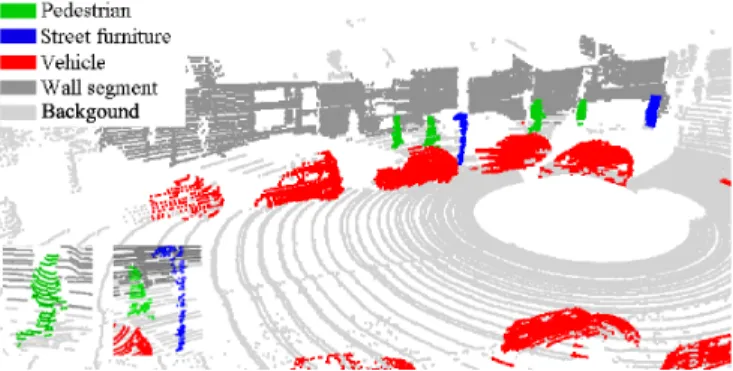
Fig. 1. Object classification result on urban point cloud using deep learning and contextual analysis. Classified objects are displayed with different colors.
the vehicles, pedestrians, trees and further street objects often occlude each other causing partially extracted object blobs in the recorded measurement streams.
A number of papers address object recognition from RMB Lidar frames. In [7] an object detection technique is intro-duced, where the classification is based on a simple shape analysis of the bounding boxes. The method of [8] uses a Sup-port Vector Machine classifier relying on a set of object level and point level features, implementing a binary vehicle/non-vehicle classification. A well-known public database is the KITTI [1], which is used by various methods [9] for quan-titative evaluation. Here a limitation is that the ground truth annotation only concerns the Field-of-View (FoV) of the forward looking cameras, which is only a segment of the 360◦ FoV of RMB Lidar scanners. If long object tracks can be extracted temporal information can be efficiently exploited in object recognition [10], but in crowded situations decision should be often made from a single time frame, immediately after a sudden appearance of an object. [11] proposed a feature learning technique for urban object recognition, and published a reference database of 588 objects from 14 different categories. However, it remains there an open issue, how the quality of the object extraction step effects the classification results, and for some object classes only a few test examples are provided. Voxel based approaches allow to perform a detailed interpretation of the scene [9], however here the computational requirements are proportional to the number of voxels and it is less straightforward to incorporate global contextual descriptors to a voxel-based local decision process. In this paper we present an end-to-end manner on object extraction and classification, where the classifier is specifically designed to efficiently process the output of our proposed fast object detector module [12]. The new algorithmic elements are evaluated step-by-step and comparison against a reference method is provided at the end.
(a) Height measurement artifact (b) 2-level grid Fig. 2. Demonstration of wall height measurement, and the hierarchical grid
II. WORKFLOW OF THE PROPOSED MODEL
The proposed approach aims to detect and localize all vehicles and pedestrians in the proximity of the mobile Lidar platform, as shown in Fig 1. The workflow consists of four consecutive steps. First, the input point cloud is segmented into four regions: ground, low foreground, high foreground and sparse areas. Low foreground is the estimated region of short street objects, such as cars, pedestrians, benches, mail boxes, billboards etc, while high foreground covers tall objects, among others building walls, trees, traffic signs and lamp posts. Following the segmentation, ground and sparse areas are removed, as they are not used by the further processing steps. Second, both the low and high foreground regions are divided into connected blobs representing individual object candidates. Third, objects extracted from the low foreground region undergo an appearance based classification, which provides evidences for discriminating vehicles and pedestrians from other street entities. In parallel, large facade segments - called as anchor facades - are detected within the high foreground’s object set. Fourth, the classification result of the previous purely appearance based step is refined with contextual information, considering the relative positions of the various sorts of short objects and anchor facades. A. Point Cloud Segmentation
Point cloud segmentation is achieved by a grid based approach [12]. We fit a regular 2-D gridSwith fixed rectangle side length onto thePz=0 plane (using the Velodyne sensor’s vertical axis as the z direction and the sensor height as a refer-ence coordinate), wheres∈Sdenotes a single cell. We assign each p∈ P point of the point cloud to the corresponding cell sp, which contains the projection of pto Pz=0. In addition, we store thezcoordinate and different height properties such as, maximum zmax(s), minimumzmin(s)and averagezˆ(s)of the elevation values within cells.
We use point height information for assigning each grid cell to the corresponding cell class. Before that, we detect and remove sparse grid cells which contains less points than a predefined threshold (used 8 points). After clutter removal all the points in a cell are classified asground, if the difference of the minimal and maximal point elevations in the cell is smaller than a threshold (used25cm), and the average elevation in the neighboring cells does not exceed an allowed height range. A cell belongs to the classhigh foreground, if either the maximal point height within the cell is larger than a predefined value (used 140cmabove the car top), or the observed point height difference is larger than a threshold (used310cm). The rest of the points in the cloud are assigned to class low foreground.
Fig. 3. The step by step demonstration of the object detection algorithm
Due to the limited vertical view angle of the Velodyne Lidar (+2◦ up to -24.8◦ down), the defined elevation criteria may fail near to the sensor position. In narrow streets where road sides located closely to the measurement position, several nearby grid cells can be misclassified regularlye.g.some parts of the walls and the building facades are classified to low foregroundcell class instead ofhigh foregroundcell class (see Fig. 2(a)). By definition, we will refer to these misclassified wall segments henceforward asshort facades, which should be detected and filtered out at a later step by the object detector. B. Object separation with fast connected component analysis After the point cloud segmentation step, our aim is to find distinct groups of points which belong to different urban ob-jects within thelowandhigh foregroundregions, respectively. For this task we use the hierarchical grid model (Fig. II-B) introduced first in [12]: On one hand, the coarse grid resolution is appropriate for a rough estimation of the 3-D blobs in the scene, in this way we can also roughly estimate the size and the location of possible object candidates. On the other hand, using a dense grid resolution beside a coarse grid level, is efficient for calculate point cloud features from a smaller subvolume of space, therefore we can refine the detection result derived from the coarse grid resolution. Although the standard 2-D grid structure from Sec. II-A could also be used for connected component extraction, that approach is not accurate enough near to the object boundaries, and does not perform well in case of nearby urban objects [12].
The following 2-level grid based connected component algorithm is separately applied for the sets of grid cells labeled as short and tall objects, respectively. First, we visit every cell of the coarse grid and for each cell s we consider the cells in its3×3 neighborhood (see Fig. 3a,3b). We visit the neighbor cells one after the other in order to calculate two different point cloud features: (i) the maximal elevation value Zmax(s) within a coarse grid cell and (ii) the point cloud
density (i.e.point cardinality) of a dense grid cell.Second, our intention is to find connected 3-D blobs within the foreground regions, by merging the coarse level grid cells together. We use an elevation-based cell merging criterion to perform this step.ψ(s, sr) =|Zmax(s)−Zmax(sr)|is a merging indicator,
which measures the difference between the maximal point elevation within cell s and its neighboring cell sr. If the ψ
indicator is smaller than a predefined value, we assume thats andsrbelong to the same 3-D object (see Fig. 3c).Third, we
perform a detection refinement step on the dense grid level. The elevation based cell merging criterion on the coarse grid level often yields that nearby and self-occluded objects are
objects, which were erroneously merged at the coarse level, could be often appropriately separated at the fine level.
C. Appearance based object recognition
Our next main goal is to identify the vehicle and pedestrian objects among the set of connected point cloud segments ex-tracted in Sec. II-B. Our general assumption is that the focused two object classes are part of the low foreground regions, therefore we start with an appearance based classification of the previously obtained short object candidates.
1) Short objects: Our labeling considers four object classes. Apart from the vehicle and pedestrian classes, we create a separate label for the short facades, which appear in the low foreground due to the limitations of the height measurement (Fig. 2a). The remaining short street objects (benches, short columns, bushes etc) are categorized as street clutter. Object recognition is performed in a supervised approach: 2D range images are derived from the object candidates, which are classified by a deep neural network. The classification output for each input point cloud sample consists of four confidence values estimating the class membership probabilities for vehi-cles, pedestrians, short facades and street clutter, respectively. To obtain the feature maps, we convert the object point clouds into regularly sampled depth images, using a similar principle to [11], but with implementing a number of differ-ences. First, we attempt to ensure side-view projections of the objects, by estimating the longitudinal cross section of the object shapes. Here using Principal Component Analysis, we calculate the two major principal vectors of the objects’ 3-D blobs, v1 and v2, which correspond to the first and second larges eigenvalues, respectively. We also use an explicit up vectorvup taken as the local ground’s normal. Thereafter, the nproj normal of the depth image’s projection plane is defined by the vector product nproj=v1×vup if the angle between v1andvupis greater than45◦ (wideobjects such as vehicles), otherwise nproj=v2×vup (thin objects like pedestrians and short poles). Second, we calculate the distance between the estimated plane and the points of the object candidate, which can be interpreted here as a depth value. In order the avoid occlusions between overlapping regionsi.e.multiple 3-D point projections into a same pixel of an image plane with different depth values, we sort the depth values in an ascending order, and we project them to the image plane starting from to closest to the farthest. As demonstrated in Fig. 4 this projection strategy ensures that object points in the front side do not become occluded by the object points in the back.
For object recognition, we trained a Convolutional Neu-ral Network (CNN) based feature learning framework called Theano firstly introduced by [13]. The CNN framework re-ceives the previously extracted depth images as an input layer scaled for the size of 96 ×96, and the outputs are four confidence values from the [0,1] range, describing the fitness
Fig. 4. Examples of depth images generated by our depth projection method.
of match to the four considered classes: vehicle, pedestrian, short facade and street clutter. In this way, we can later utilize not only the index of the winner class, but also describe how sure the CNN module was about its decision for a given test sample. After testing various different layer configurations, we experienced that four pairs of convolution-pooling layers followed by a fully connected dense layer give us the most efficient results.
2) Tall objects: The car-mounted horizontal RMB Lidar configuration is generally not well suited the recognition and analysis of tall field objects (e.g. traffic lights, high-mounted traffic signs), since their upper parts lie often out of the vertical field of view of the sensor. In this paper, we do not focus on the discrimination of these objects, but we extract the large facade segments from thehigh foregroundregions, which will be used as reference points in contextual analysis of the scene in Sec. II-D. These facade segments are typically elongated objects, thus their detection is simply based on the length measured in the principal direction of the 3-D point cloud blob. We call henceforward the wall segments extracted in this way as anchor facades, because we can roughly model the street boundaries relying on them.
D. Contextual labeling refinement
The object classification step of Sec. II-C recognizes the street entities purely based on appearance features extracted from the individual objects, without considering any other scene elements. However, since among the recognizable tar-gets we must expect the presence of occluded and only partially extracted object segments, the sample shapes from the different classes may be often confused. Most frequently, we have experienced that the CNN based classification module confuses severalvehicleswithsort facadesdue to their similar size and shape parameters. For eliminating these artifacts, we extended our approach with a contextual refinement step, exploiting topological relations between various scene objects. Typically the following three situations should be handled:
• Objects with similar shapes to vehicles or street furniture elements may appear between the building wall segments, which errors can be corrected through alignment compar-ison of theshort objectcandidates (from Sec. II-C1) and theanchor facades (from Sec. II-C2).
Fig. 5. Contextual analysis: calculating the object-anchor facade alignment distance feature
• Some objects in the middle of the road may have very similar (usually high) CNN confidence values both for the vehicle and short facade classes. This case typi-cally appears if two closely passing cars are erroneously merged by the object detector (Sec. II-B), or the vehicle’s observed shape is atypical from the Lidar’s viewpoint. • Long vehicles with large side surfaces (such as trucks
and trams) are usually classified as facades with a high confidence gap against thevehicleclass. We have experi-enced that due to the data sparsity these cases cannot be efficiently separated at object appearance level, thus we should rely here on the scene topology.
The contextual analysis module receives as input the sets of anchor facades and short object candidates, where each short object is assigned to the four class confidence values (vehicle, pedestrian, short facade and street clutter), and an initial class label corresponding to the class with the highest confidence by the CNN classifier. Beside appearance related properties, we define a topological feature, called alignment distance, between the detected short objects and anchor facades. The calculation of the dalignment distance term is demonstrated in Fig. 5, showing an anchor facadef, and two short objectso ando∗. Let us consider thed(o, f)distance first. Using PCA, we derive the main axesaf andao of the object blobsf and
o respectively. We determineP1 andP2 as the two boundary points of o along the axisao. Letd1 andd2 be the distances
of P1 andP2 from af, and taked(o, f) = d1+2d2. Similarly,
d(o∗, f) = d∗1+d∗2
2 . In this example, the alignment distance feature suggests that based on scene topology, o might be a real vehicle, and o∗ a facade segment.
The step of context based re-classification of short objects is detailed by Algorithm 1, whereIsConfident(oi) is a boolean
function returning true iff for oi the ratio of the first and
second largest CNN confidence values is larger than 0.8. III. EXPERIMENTALRESULTS ANDEVALUATION
Since our method implements an end-to-end pipeline from object perception until recognition, the public Sydney [11] and Stanford [10] databases are in themselves inappropriate for validating the proposed approach. We could neither use KITTI benchmark, since some of our examined issues, such as the short facade artifacts appear in the side view segment of the 360◦ FoV of the car-mounted Lidar, which regions are not annotated by KITTI. For this reason, we created a new hand labeled dataset, called SZTAKI Velo64Road,
Fig. 6. Comparison of the appearance based and the combined model Input:Set of pre-labeled short objectsO={o1, o2, . . . , on} Input:Set of anchor facadesF ={f1, f2, . . . , fm}
Output: Objects with modified labelsO={o1, o2, . . . , on} fori←1tondo
ifminf∈Fd(oi, f) < µ then Label(oi) ←Facade
else ifLabel(oi) = Facadethen if!IsConfident(oi)then Label(oi) ←Vehicle else Label(oi) ←LongVehicle end returnO={o1, o2, . . . , on}
Algorithm 1: Object’s class label modification according to contextual information.
based mainly on point cloud sequences recorded by our car-mounted Velodyne HDL-64 Lidar scanner in the streets of Budapest, Hungary1. First we run the segmentation (Sec. II-A) and object extraction (Sec. II-B) steps of our model on the raw data, thereafter we annotated all the automatically extracted short objects (2063 objects alltogether) without any further modification with the labelsvehicle,pedestrian,short facadeandstreet clutter. In this way the analyzed objects are represented by point cloud segments obtained by a realistic object extractor, and the distribution and characteristics of the artifacts caused by occlusion or varying data density reflect
1TheSZTAKI Velo64RoadBenchmark is available from the following url:http://web.eee.sztaki.hu/i4d/SZTAKI-Velo64Road-DB.html
levels.First, the object separation module (Sec. II-B) was eval-uated, by comparing the automatically extracted object blobs to a manually labeled ground truth configuration. As described in [12], we counted the true positives, missing objects and false objects, thereafter we calculated the F-rate of the detection as the harmonic mean of precision and recall. As reference of the proposed 2-level grid based model we used a 3-D connected component analysis (3D-CCN) method implemented in [15]. In F-rate the proposed approach outperformed 3D-CCN with 13% (84% vs. 71%), while it decreased the running speed by two orders of magnitude due to eliminating the kd-tree building step at each frame (27 fps vs. 0.30 fps in average, measured over 1800 sample frames).
At the second level, we focused on the final two steps of the workflow, evaluating the appearance based object labeling (Sec. II-C), and the context based refinement of the classifica-tion (Sec. II-D). For training the CNN classifier, we separated 904 objects from our dataset, which was completed with 434 selected samples of the Sydney Urban Object Dataset [11]. Thus the training set consists of 1338 objects in total, including 402 vehicles, 261 short facades, 467 street clutter elements and 208 pedestrians. The test data contains 1485 objects overall, including the remaining 1159 objects of theSZTAKI Velo64 dataset (588 vehicles, 72 short facades 452 street clutter samples and 77 pedestrians), and 326 objects from the Washington dataset (126 vehicles, 65 short facades, 101 street clutter samples and 34 pedestrians). During the evaluation we counted the correctly and erroneously classified objects, and based on the calculated confusion matrix we derived the precision, recall and F-rate values of the detection for each class separately and cumulatively as well. Results of the appearance based detection step and the context based refinement step can be compared in Table I. We can observe a significant improvement regarding the classification accuracy of vehicles and short facades, especially by the large decrease of the false hits instead of wall segments. As an independent reference technique, we considered here an object matching algorithm based on corresponding grouping from [15], which compares the detected 3-D object candidates to verified sample objects from the training data to decide their classes. A similar approach was followed in [4] for classifying urban objects from street scenarios from dense Mobile Laser Scanning data. As shown Table I, the object matching process [15] can also be adopted to the significantly sparser RMB Lidar point clouds, but its performance is about 15% weaker compared to our proposed method, which presents an 89% overall F-rate. Following [9], we also calculated the avg precision of the proposed model, and observed similar values to [9]:0.52 for vehicles and 0.46for pedestrians.
IV. CONCLUSION
We have proposed an end-to-end pipeline of fast object extraction and classification from sparse point clouds, for
SF 137 79 52 62 82 63 71 93 77 84
SC 553 87 93 90 91 96 93 92 97 94
P 111 66 57 61 78 75 77 78 78 78
Sum 1485 76 72 74 86 83 85 90 87 89
Notations: Object categories (OC): Vehicle (V), Short facades (SF), Street clutter (SC), Pedestrian (P), Number of objects (NO), Precision (Pr), Recall (Rc), F-rate (Fr), in %
the purpose of vehicle and pedestrian detection in urban environments, with jointly utilizing deep learning based object appearance models and contextual scene analysis. The method was validated on real measurements of a rotating multi-beam Lidar sensor, and the efficiency was compared to a baseline technique. The authors thank L. Kov´acs and D. Varga for advices in deep learning.
REFERENCES
[1] A. Geiger, P. Lenz, and R. Urtasun, “Are we ready for autonomous driving? the kitti vision benchmark suite,” inConference on Computer Vision and Pattern Recognition (CVPR), 2012.
[2] A. B¨orcs, B. Nagy, and C. Benedek, “Dynamic environment perception and 4D reconstruction using a mobile rotating multi-beam Lidar sensor,” inHandling Uncertainty and Networked Structure in Robot Control, ser. Studies in Systems, Decision and Control. Springer, 2016, pp. 153–180. [3] B. Yang and Z. Dong, “A shape-based segmentation method for mobile laser scanning point clouds,” ISPRS Journal of Photogrammetry and Remote Sensing, vol. 81, pp. 19 – 30, 2013.
[4] Y. Yu, J. Li, J. Yu, H. Guan, and C. Wang, “Pairwise three-dimensional shape context for partial object matching and retrieval on mobile laser scanning data,”IEEE Geoscience and Remote Sensing Letters, vol. 11, no. 5, pp. 1019–1023, May 2014.
[5] B. Yang, Z. Dong, G. Zhao, and W. Dai, “Hierarchical extraction of urban objects from mobile laser scanning data,”ISPRS Journal of Photogrammetry and Remote Sensing, vol. 99, pp. 45 – 57, 2015. [6] J. Behley, V. Steinhage, and A. B. Cremers, “Performance of histogram
descriptors for the classification of 3D laser range data in urban environ-ments.” inIEEE International Conference on Robotics and Automation (ICRA), St. Paul, MN, USA, 2012, pp. 4391–4398.
[7] A. Azim and O. Aycard, “Detection, classification and tracking of moving objects in a 3D environment.” in IEEE Intelligent Vehicles Symposium (IV), Alcal´a de Henares, Spain, 2012, pp. 802–807. [8] M. Himmelsbach, A. M¨uller, T. Luettel, and H.-J. Wuensche,
“LIDAR-based 3D Object Perception,” inInternational Workshop on Cognition for Technical Systems, Munich, Germany, 2008.
[9] D. Z. Wang and I. Posner, “Voting for voting in online point cloud object detection,” inProc. of Robotics: Science and Systems, Rome, Italy, 2015. [10] A. Teichman, J. Levinson, and S. Thrun, “Towards 3D object recognition via classification of arbitrary object tracks,” inInternational Conference on Robotics and Automation, 2011.
[11] M. De Deuge, A. Quadros, C. Hung, and B. Douillard, “Unsupervised feature learning for outdoor 3D scans,” Proceedings of Australasian Conference on Robotics and Automation, 2013.
[12] A. B¨orcs, B. Nagy, and C. Benedek, “Fast 3-D urban object detection on streaming point clouds,” inWorkshop on Computer Vision for Road Scene Understanding and Autonomous Driving at ECCV 2014, ser. LNCS, Z¨urich, Switzerland, 2015, vol. 8926, pp. 628–639.
[13] F. Bastien, P. Lamblin, R. Pascanu, J. Bergstra, I. J. Goodfellow, A. Bergeron, N. Bouchard, and Y. Bengio, “Theano: new features and speed improvements,” in Deep Learning and Unsupervised Feature Learning Workshop at NIPS, Lake Tahoe, USA, 2012.
[14] K. Lai and D. Fox, “Object recognition in 3D point clouds using web data and domain adaptation,”Int. J. Rob. Res., vol. 29, no. 8, pp. 1019– 1037, Jul. 2010.
[15] R. B. Rusu and S. Cousins, “3D is here: Point cloud library (PCL),” in