Research papers
Evaluation of a physically based quasi-linear and a conceptually based
nonlinear Muskingum methods
Muthiah Perumal
a, Gokmen Tayfur
b,⇑, C. Madhusudana Rao
c, Gurhan Gurarslan
d aDepartment of Hydrology, Indian Institute of Technology Roorkee, Roorkee 247667, Indiab
Department of Civil Engineering, Izmir Institute of Technology, Izmir, Turkey c
Department of Civil Engineering, National Institute of Technology Jamshedpur, Jamshedpur 831014, India d
Department of Civil Engineering, Pamukkale University, Denizli, Turkey
a r t i c l e i n f o
Article history:Received 5 August 2016
Received in revised form 22 December 2016 Accepted 15 January 2017
Available online 21 January 2017 This manuscript was handled by Corrado Corradini, Editor-in-Chief Keywords: Open channel Flood routing Conceptual Nonlinear
Variable parameter Muskingum method Artificial intelligence methods
a b s t r a c t
Two variants of the Muskingum flood routing method formulated for accounting nonlinearity of the channel routing process are investigated in this study. These variant methods are: (1) The three-parameter conceptual Nonlinear Muskingum (NLM) method advocated by Gillin 1978, and (2) The Variable Parameter McCarthy-Muskingum (VPMM) method recently proposed by Perumal and Price in 2013. The VPMM method does not require rigorous calibration and validation procedures as required in the case of NLM method due to established relationships of its parameters with flow and channel char-acteristics based on hydrodynamic principles. The parameters of the conceptual nonlinear storage equa-tion used in the NLM method were calibrated using the Artificial Intelligence Applicaequa-tion (AIA) techniques, such as the Genetic Algorithm (GA), the Differential Evolution (DE), the Particle Swarm Optimization (PSO) and the Harmony Search (HS). The calibration was carried out on a given set of hypo-thetical flood events obtained by routing a given inflow hydrograph in a set of 40 km length prismatic channel reaches using the Saint-Venant (SV) equations. The validation of the calibrated NLM method was investigated using a different set of hypothetical flood hydrographs obtained in the same set of chan-nel reaches used for calibration studies. Both the sets of solutions obtained in the calibration and valida-tion cases using the NLM method were compared with the corresponding soluvalida-tions of the VPMM method based on some pertinent evaluation measures. The results of the study reveal that the physically based VPMM method is capable of accounting for nonlinear characteristics of flood wave movement better than the conceptually based NLM method which requires the use of tedious calibration and validation procedures.
Ó2017 Elsevier B.V. All rights reserved.
1. Introduction
The objective of channel flood routing is to track the movement of flood wave while it propagates from an upstream section to a downstream section in a channel reach. Flood routing analysis is required for various purposes such as flood forecasting, design of flood protection structures and for estimation of spillway design flood. A variety of channel routing methods have been proposed in the literature (Fread, 1993) and they can be broadly classified into two major categories as (i) hydraulic routing and (ii) hydro-logic routing. The hydraulic routing methods can be further classi-fied as dynamic routing and simpliclassi-fied hydraulic routing. The
hydrologic routing method is widely used in field practices since early thirties and they have been developed essentially to over-come the tedious computations involved in the hydraulic routing methods. This method treats the channel reach as a lumped system and employs the lumped continuity equation, derived from the dis-tributed continuity equation of the Saint-Venant (SV) equations (Saint-Venant, 1871a, 1871b), and a storage equation formulated by linking the reach storage with the inflow and outflow variables of the routing reach. Among the many lumped hydrological routing
methods, the Muskingum method introduced byMcCarthy (1938)
is well known in the literature (Chow et al., 1988). McCarthy (1938)introduced this classical method as a linear storage routing method wherein the reach storage at any instant of time is linearly related to the linear weighted discharge expressed in terms of inflow and outflow involving two parameters. Recognizing the inability of the classical Muskingum method to account for
nonlin-http://dx.doi.org/10.1016/j.jhydrol.2017.01.025
0022-1694/Ó2017 Elsevier B.V. All rights reserved. ⇑ Corresponding author.
E-mail addresses:[email protected](M. Perumal),[email protected]. tr(G. Tayfur),[email protected](C.M. Rao),[email protected]. tr(G. Gurarslan).
Contents lists available atScienceDirect
Journal of Hydrology
ear characteristics of flood wave movement in channels,Gill (1978)
advocated an approach of accounting nonlinearity in the channel routing process by modifying the storage equation of the classical Muskingum method in nonlinear form by expressing the linear weighted discharge with a nonlinear exponent.Gill (1978)named this method as the Nonlinear Muskingum (NLM) method to differ-entiate it from the linear classical Muskingum method. Parallel to the development of the NLM method, an alternate approach of accounting nonlinearity by the Muskingum method was studied by Ponce and Yevjevich (1978)resulting in the development of Variable Parameter Muskingum-Cunge (VPMC) method. The VPMC method is an extension of the Muskingum-Cunge (MC) method
developed by Cunge (1969) by relating the parameters of the
Muskingum method with flow and channel characteristics using the matched diffusivity approach. Though both the NLM and VPMC methods were developed with the objective of overcoming the deficiency of the classical Muskingum method for its inability to account for nonlinearity in the channel routing process, the approach of accounting nonlinearity by these methods differ from each other. In the case of NLM method, the structure of the storage equation expressed in the nonlinear form of the linear weighted discharge is universal, but the parameters of the storage equation employed remain constant for the considered event which need to be calibrated using site specific recorded inflow and the corre-sponding outflow hydrographs. Though the NLM method charac-terized by an additional parameter has increased the flexibility of the method better than the classical Muskingum method in closely simulating the observed hydrograph of the calibration flood event, the set of parameters calibrated may not be able to simulate other flood events for lower or higher range of flow than the one used in the calibration for the same channel reach. However, the VPMM method does not exhibit such a deficiency as the parameters vary nearly in a manner consistent with the variability built-in in the
flood wave propagation process. Following the studies of Gill
(1978), andPonce and Yevjevich (1978)a number of studies have been carried out by various researchers for accounting nonlinearity in the routing process by these two variant Muskingum routing methods. Most of the studies conducted on the NLM method relate to various methods of parameter estimation based on a plethora of optimization techniques such as those proposed byTung (1985), Yoon and Padmanabhan (1993), Mohan (1997), Geem (2006a)
andKarahan et al. (2013). But none of these studies ever followed the conventional modelling protocol involving calibration and val-idation of the method. Followed by the development of VPMC method, a number of Variable Parameter Muskingum (VPM) meth-ods have been proposed in the literature. These methmeth-ods enable to relate the Muskingum parameters in a manner more consistent with the variability built-in the channel routing process better than the approach advocated byPonce and Yevjevich (1978). Fur-ther these VPM methods have been also developed with the objec-tive of overcoming the mass conservation problem associated with
the VPMC method (Perumal and Sahoo, 2008). Notable among
these methods are due to Todini (2007), Price (2009), and
Perumal and Price (2013). It may be pointed out that though a par-allel development on these two approaches of accounting nonlin-earity in the routing process by the Muskingum method have been made, no investigation has been made so far to demonstrate the comparative evaluation of the performances of the NLM method and the VPM methods. Therefore, this study is made with the following objectives: (1) to assess the performance of the NLM method first by calibrating the parameters of the method using some selected Artificial Intelligent Algorithm (AIA) techniques on the given set of flood events and subsequently validating the method by simulating the outflow hydrographs used for the cali-bration of the method, and (2) to compare the performances of the NLM and VPMM methods in reproducing the pertinent
characteristics of the benchmark hydrographs of the independent set of flood events considered as the validation events. It may be noted that the VPMM method does not require the calibration of parameters as they have established relationships with channel and flow characteristics. Further, it may also be pointed out that any of the volume conservative variable parameter Muskingum
methods, such as the method proposed byTodini (2007), Price
(2009) and Perumal and Price (2013) could have been used as the candidate method of the physically based variable parameter Muskingum method as all of these methods perform with the same level of accuracy (Price, 2009;Perumal and Price, 2013). The VPMM method is used in this study due to its familiarity with the authors. This paper is organized as follows: Section2describes the clas-sical and nonlinear Muskingum methods, and the variable param-eter Muskingum method, specifically the VPMM method. Section3
describes the calibration of the NLM method using some selected AIA techniques, such as the Genetic Algorithm (GA), the Differen-tial Evolution (DE), the Particle Swarm Optimization (PSO) and the Harmony Search (HS). Section4gives the description of hypo-thetical inflow hydrographs used for arriving at the routed hydro-graphs, which are considered as benchmark solutions, required for both calibration and validation studies in the considered channel reaches. These set of hypothetical inflow and outflow hydrographs are used for parameters calibration of the selected AIA techniques employed in the NLM method and their subsequent validation. These set of hydrographs are also employed for simulation using the VPMM method for subsequent comparative evaluation with the simulations of the NLM method. The hypothetical channel reaches characterized by different channel configurations used in the study are also described in this section. Section5gives the details of the numerical experiments conducted for the study and the strategy adopted for the comparative evaluation of the
simula-tion performances of the NLM and VPMM methods. Secsimula-tion6
pre-sents the results and discussion of the study based on the obtained simulation results, and the conclusions of the study are presented in Section7.
2. Various forms of the Muskingum method
2.1. The classical Muskingum routing method
The classical Muskingum method (McCarthy, 1938) of flood
routing derived its name after its first application to the Musk-ingum River, a tributary of the Ohio River in the USA, is a linear storage routing method and it is widely used in practice (Chow et al., 1988). This method models the flood storage of a given rout-ing reach at any instant of time of the propagation of a flood event as a combination of wedge and prism storage. This method combi-nes the lumped continuity equation
dS
dt¼IO ð1Þ
with a linear storage equation expressed as
S¼K½hIþ ð1hÞO ð2Þ
to arrive at the difference equation which on simplification leads to the Muskingum routing equation as
Ojþ1¼C1Ijþ1þC2IjþC3Oj ð3Þ
whereSis the storage volume,Iis the inflow discharge,Ois the out-flow discharge,Kis the travel time,his the weighting parameter, the suffixjdenotes the timejDt, where,Dtis the routing time step, and the routing coefficients C1, C2, and C3are expressed as C1¼
Khþ0:5t
C2¼ Khþ0:5t Kð1hÞ þ0:5t; ð4bÞ C3¼ Kð1hÞ 0:5t Kð1hÞ þ0:5t; ð4cÞ
where C1+ C2+ C3= 1 which shows the mass conserving ability of the classical Muskingum method. Given an inflow hydrograph, an initial flow condition, a chosen time stepDt, and the routing param-etersKandh, the routing coefficients can be calculated using Eq. (4) and used subsequently to arrive at the outflow hydrograph using Eq.(3). The routing parametersKandhare implicitly related to flow and channel characteristics withKbeing interpreted as the travel time of the flood wave from upstream end, where the inflow hydro-graph is applied, to the downstream end of the routing reach. The
parameter h is the weighting parameter used for weighting the
prism and wedge storages to determine the equivalent prism stor-age of the reach at any instant of time. To calculate the value ofh, the storageS is plotted against the corresponding weighted dis-charge value [hI+ (1h)O] in Eq.(2)for different trial values ofh resulting in various sizes of loops; and the value ofhwhich gives the narrowest loop of this plot is considered as the appropriate one for its use in the method. The effect of storage is to reduce the peak flow and spread the hydrograph over time and this effect introduces diffusion of the propagating flood wave resulting in peak attenuation. The successful application of the Muskingum method for real life routing problems led the hydrologists to consider that there exists some link between the parametersK andh, and the channel and flow characteristics. Subsequently several attempts have been made by various researchers (Dooge and Harley, 1967; Cunge, 1969; Dooge et al., 1982) to link the routing parametersK andhof the classical Muskingum method with the flow and channel characteristics based on the hydrodynamics principles to transform it into a physically based method. Further, various attempts have been made for the physical interpretation of the classical Musk-ingum method by several researchers likeApollov et al. (1964), Cunge (1969), Dooge (1973), Koussis (1976), Strupczewski and Kundzewicz (1980), Dooge et al. (1982), Kundzewicz (1986), Perumal (1992, 1994), andPonce and Chaganti (1994).
2.2. Nonlinear Muskingum (NLM) method
Recognizing the inability of the classical Muskingum method for modeling nonlinear behavior of flood wave movement in chan-nels,Gill (1978)advocated an alternative approach of accounting nonlinearity in the channel routing process by expressing the stor-age equation of the classical Muskingum method in nonlinear form simply by raising the weighted discharge by an exponent ‘m’ expressed in the following form:
SðtÞ ¼K½hIðtÞ þ ð1hÞOðtÞm ð
5Þ
In addition to the two parameters employed in the classical Muskingum method, Gill’s storage equation employs a third parameter in the form of nonlinear exponentm.Gill (1978)named this method as the nonlinear Muskingum (NLM) method. When m =1, the storage equation of the NLM method reduces to the stor-age equation of the classical Muskingum method.
It may be noted that an increase of one more parameter ‘m’ associated with the modified form of the storage equation of the NLM method increases the flexibility of the method in closely sim-ulating the observed outflow hydrograph of the calibration flood event. However, the close reproduction of outflow hydrograph achieved in the calibration mode does not guarantee the set of esti-mated calibration parametersK,handmto be universal or global optimal parameters for the considered channel reach for simulat-ing all the possible flood hydrographs that may be routed in that
channel reach. This is due to the reason that a set of calibrated parameters estimated using one of the recorded set of flood events in a routing reach is not only influenced by the channel character-istics, but also by the inflow hydrograph characteristics such as the shape, peak, its rate of rise and time to peak, besides the prevailing initial flow in the channel reach. If a flood event of a higher or lower magnitude with differing inflow hydrograph characteristics and with a different prevailing initial flow in the reach, other than that of the past calibrated event, is to be routed in the same chan-nel reach, then the parameters calibrated from the past event may not serve the intended purpose of successfully reproducing the observed hydrograph by routing this new inflow hydrograph.
2.3. Variable Parameter McCarthy-Muskingum (VPMM) method
Perumal and Price (2013)recently proposed a physically based variable parameter Muskingum method developed from SV equa-tions. This method was developed with the objectives of account-ing non-linearity in the routaccount-ing process and for fully conservaccount-ing mass of the routed hydrograph. The development of the method justifies the heuristic assumption used byMcCarthy (1938)in the classical Muskingum method that the reach storage consists of prism and wedge storages. In a way of recognizing the contribution ofMcCarthy (1938)for the development of the well-known
Musk-ingum method,Perumal and Price (2013)named this method as
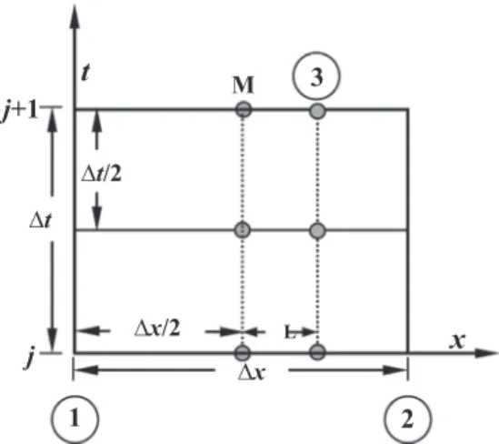
the Variable Parameter McCarthy-Muskingum (VPMM) method. The VPMM method uses the approximate form of the momen-tum equation of the SV equations in expressing discharge at the mid-section of the routing reach (seeFig. 1) as:
QM¼QoM 1 1 So @y @x 1 4 9F 2 M P B dR dy 2 M " # ( )1 2 ð6Þ wherePM,BM,FMandRM, respectively, denotes the wetted
perime-ter, top width, Froude number and hydraulic radius corresponding to the flow depthyM.
The suffix ‘M’ and the suffix ‘oM’ attached to a variable refer to that variable estimated at the mid-section of the sub-reach corre-sponding toyMand its normal discharge, respectively. Accordingly,
the notationQMis the average discharge at the mid-section of the
reach at any time (see,Fig. 1) andQoMis the normal discharge at
the midsection corresponding to flow depthyM; (@y/ox) is the
lon-gitudinal water depth gradient; andSodenotes the bed slope of the
channel or river. The Froude number FM is expressed as
FM¼
ffiffiffiffiffiffiffiffiffiffiffiffiffiffiffiffiffiffiffiffiffiffiffiffiffiffiffiffiffiffiffiffi ðQ2MBMÞ=ðgA3MÞ q
, where g denotes the acceleration due to
Δx O I 1 Q3 QM L Δx/2 yu yM y3 yd M 3 2
gravity and AM denotes the flow area of cross-section at
mid-section of the reach or subreach.
Use of the approximate expression for the normal discharge, QoM, obtained from the above equation using the binomial series
expansion and the direct use of the same in the one-dimensional continuity equation of the SVequations applied at the centre point of the box-grid scheme as shown inFig. 2results in the mass con-servative routing equation of the VPMM method expressed as (Perumal and Price, 2013):
Ojþ1¼
D
t2Kjþ1hjþ1D
tþ2Kjþ1 ð1hjþ1Þ Ijþ1þD
tþ2KjhjD
tþ2Kjþ1 ð1hjþ1Þ Ijþ Dtþ2Kj ð1hjÞD
tþ2Kjþ1 ð1hjþ1Þ Oj ð7ÞThe notationj denotes the time t=jDt and the notation Dt denotes the routing time step.
The routing parameters,Kand h at the time level (j+1) are expressed (Perumal and Price, 2013), respectively, as;
Kjþ1¼
D
x VoM;jþ1 ð8Þ hjþ1¼ 1 2 QoM;jþ1 2S0BM;jþ1coM;jþ1D
x ð9Þwhere,V =flow velocity.
The dischargeQoM,j+1is estimated as:
QoM;jþ1¼hjþ1Ijþ1þ ð1hjþ1ÞOjþ1 ð10Þ
During unsteady flow the normal discharge QoM,j+1 passes at some section located downstream of the midsection of the Musk-ingum reach and it is denoted as section-3 as shown inFig. 1. It may be noted that the VPMM method does not consider the con-cept of matching the numerical diffusion with the physical diffu-sion as in the case of the VPMC method. However, the same form of the routing equation of the classical Muskingum method is used by the VPMM method, except that the routing coefficients are esti-mated using the physically based parametersKandhwhich vary at every time step following the Eqs.(8) and (9), respectively. As the parameters remain constant over the time step Dt, but vary at every step, this method can be considered as a quasi-linear method.
Perumal and Price (2013) inferred from the development of VPMM method that it can be successfully applied for channel and river routing problems when the inflow hydrograph is charac-terized by the criterionjð1=SoÞð@y=@xÞj60:5, where Sodenotes the
channel bed slope and ð@y=@xÞ denotes the longitudinal water depth gradient.
3. Calibration of the NLM method
Ever since the introduction of the NLM method, a number of techniques for its parameter estimation have been introduced. Almost all of these parameter estimation techniques have been introduced based on the criterion of close reproduction of the observed hydrograph of the calibration event by the solution of the NLM method, though the improvement achieved in the repro-duction of the observed hydrograph of the considered calibration event by the proposed AIA technique could be considered insignif-icant over the reproductions of the same event by the methods based on the other AIA techniques. Among these techniques, the ones based on AIA techniques, such as the GA, DE, PSO and HS are considered for their application in this study. It may be noted that none of the researchers attempted to prove the claim of supe-riority of their parameter estimation technique in the validation of the calibrated model using independent set of inflow and outflow hydrographs of the same channel reach.
Depending on the type of parameter estimation technique used, such as GA, DE, PSO and HS, the parametersK,hand m of the NLM method are calibrated by minimizing the residual sum of squares between the benchmark solutions (Oobs,(t)) and the routing
solu-tionOr(t) obtained by the NLM method, expressed as:
Min SSQ¼X½OobsðtÞ OrðtÞ2 ð
11Þ
The calibration stage, in this study, involves the close reproduc-tion of the benchmark solureproduc-tion by the NLM method. The bench-mark solution (outflow hydrograph) is obtained by routing inflow hydrograph in a channel. This is achieved by the solution of St. Venant equations. During the calibration stage, while the benchmark solution is reproduced by the NLM method, the opti-mal values of the NLM method parameters (i.e.;K,handm) are obtained using the AIA methods. The validation stage, on the other hand, involves the simulation of another event by the NLM method using the parameter values obtained at the calibration stage. 3.1. Artificial Intelligence Application (AIA) techniques
3.1.1. GA method for parameter estimation
GA is an optimization algorithm which can make a nonlinear search in a solution space such that the continuity (and conse-quently the differentiability) of the underlying mathematical func-tion is not necessary. Furthermore, it makes few assumpfunc-tions and therefore it is robust and it has general applicability (Liong et al., 1995; Goldberg, 1999).
GA has four basic units:bit,gene,chromosome, andgene pool.Bit is the basic element which is represented by a 1 (or) 0 digit. The combination of bits forms agenewhich represents a model param-eter (or a decision variable). The attachment of genes forms a chro-mosomewhich stands for a possible solution.
GA algorithm have four basic operations: generating initial gene pool, obtaining fitness for each chromosome, selection of somes, cross-overing chromosomes, and ‘mutuating chromo-somes’. Uniform distribution (or a normal distribution) (Sen, 2004) can be employed to randomly generate initial chromosomes for the gene pool. Fitness of each chromosome can be evaluated in two steps: First, substituting each chromosome into objective function to find their values; and then, obtaining their fitness by Eq.(12)(Tayfur, 2012): FðCiÞ ¼PfðCiÞ fðCiÞ ð12Þ
x
M
t
∆
x
L∆
t
/2
2
1
3
∆
x
/2
j
j
+1
∆
t
Fig. 2.Numerical grid adopted for VPMM application in synchronization with
whereCiis chromosomei; f(Ci) is value of objective function for
chromosomei, andF(Ci) is fitness value for chromosomei.
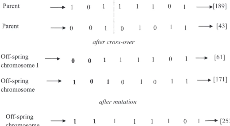
Selection of chromosomes after the evaluation of their fitness values can be performed randomly. There are methods available for the selection process such as roulette wheel (Sen, 2004) and ranking (Tayfur, 2012). After the selection process, pairs (parent chromosomes) are first formed and they are then subjected to the cross-over operation by interchanging the genes. The last oper-ation in a single iteroper-ation is the mutoper-ation by which bits are reversed (i.e.,1 to 0or0 to 1). By these operations, it is intended to search the solution space thoroughly. As an example,Fig. 3
shows mutation and single cut cross-over operations. As seen, the first two chromosomes (parent chromosomes I and II) are sub-jected to the cross-over by the single cut from the third digit, yield-ing new chromosomes (off-spryield-ings I and II) at the bottom. The value of 189 becomes 61 after cross-over and then 253 (off-spring chromosome III) after mutation, thus scanning a large por-tion of solupor-tion space. One can find more details on GA in (Goldberg, 1999; Sen, 2004; Tayfur, 2012).
This study employed Evolver (Palisade Corporation, 2013) soft-ware package for estimating the parameters (K,h,m) of the nonlin-ear Muskingum method. The parameters are first assigned random values before initiating the iterations. Note that the initial assigned values do not affect the final convergence of the results. 100 chro-mosomes in the initial gene pool, 75% cross-over rate, 5% mutation rate and 10000 iterations were employed.
The parameters were calibrated for each event in the consid-ered channel reaches whose slope varied between 0.001 and 0.0001 with the same inflow hydrograph peak rate of 800 m3/s (10 different events). The so-obtained optimal values of the param-eters are summarized inTable 1. The NLM method calibrated based on the GA technique was then verified using the independent sets of inflow and the corresponding benchmark outflow events arrived at in the respective channel systems used for calibration, but using an inflow hydrograph nearly same as the one employed in the cal-ibration exercise. The details of the inflow hydrographs used for calibration and validation studies are described later.
3.1.2. DE method for parameter estimation
DE is an evolutionary optimization method which is simple, fast, robust and powerful in finding global optimum (Storn and Price, 1997). Like GA, it is a population based and uses similar operations such as selection, crossover, and mutation. The basic difference between GA and DE is that GA relies more on crossover while DE on mutation, as a search mechanism. Selection operation in DE is employed to direct the search towards the prospective
regions in the solution space. Non-uniform crossover is used in DE algorithm, by which child vector parameters are taken more often from one parent. In DE, the population of NP solution vectors is randomly created at the beginning and successfully improved by applying mutation, crossover and selection operators (Karaboga and Okdem, 2004). Normally,NP should be about 10 times the
number of parameters in a vector (Storn and Price, 1997;
Karahan, 2011).
A mutant vector can be produced by DE/rand/1/bin strategy for each target vectorXi;j;Gas follows (Storn and Price, 1997):
Vi;j;Gþ1¼XR1;j;GþFðXR2;j;GXR3;j;GÞ: ð13Þ where j2 f1;2;. . .;Dg;i;R1;R2;R32 f1;2;. . .;NPg are randomly chosen and must be different from each other,Gis the generation number. In Eq.(13),Fis the mutation factor which has an effect on the difference vector (XR2,j,GXR3,j,G).
A trial vector can be produced by mixing the parent vector with the mutated vector as:
Ui;j;Gþ1¼
Vi;j;Gþ1; if randj6 CR or j 6j rand
Xi;j;G; if randj>CR or j–j rand
ð14Þ
where j
e
{1, 2,. . ., D};randje
[0, 1] is the random number; CRe
[0, 1] is crossover rate andjrand
e
{1, 2,. . ., D} is the randomly cho-sen index.All chromosomes in the population have the same chance for being selected as parents, irrespective of their fitness values. The child, produced after the mutation and crossover operations, is first evaluated. Then, the better one is chosen after comparing the per-formances of the child vector and its parent. If the parent is still better, it is retained in the population by the following:
Xi;j;Gþ1¼
Ui;j;Gþ1; fðUi;j;Gþ1Þ<fðXi;j;Gþ1Þ
Xi;j;G; otherwise
ð15Þ
The details of DE can be obtained from the literature (Storn and Price, 1997; Karaboga and Okdem, 2004; Karahan, 2011; Vasan and Simonovic, 2010; Gurarslan, 2011). The parameters were cali-brated by DE for each event (Table 1) and tested against other 10 events.
3.1.3. PSO method for parameter estimation
PSO method is also a population based evolutionary search opti-mization method inspired from the movement of bird flock (swarm) (Chau, 2007; Clerc and Kennedy, 2002). Although it is similar to GA with respect to fitness concept and random popula-tion initializapopula-tion, the evolupopula-tion of generapopula-tions in such a system occurs by cooperation and competition. The population responds
[189] 1 0 1 [43] [171] 1 1 1 1 0 1 [253] Parent 1 Parent Off-spring chromosome I Off-spring chromosome 1 Off-spring chromosome 1 0 1 1 1 0 0 1 0 1 0 1 0 0 1 1 1 1 0 0 0 1 1 1 0 1 1 after cross-over 1 [61] 1 after mutation
to the quality factors of the previous best individual and group val-ues. It is adaptive corresponding to the change of the best group value and fast convergent (Chau, 2007; Kumar and Reddy, 2007).
The basic idea in PSO is based on the assumption that potential solutions are flown through hyperspace with acceleration towards more optimum solutions. Each particle adjusts its flying according to the experiences of both itself and its companions. During the process; the overall best value attained by all the particles within the group and the coordinates of each element in hyperspace asso-ciated with its previous best fitness solution are recorded in the
memory (Chau, 2007; Kumar and Reddy, 2007). The important
advantage of PSO algorithm is its relatively simple coding and low computational cost (Chau, 2007).
Mathematical statement of PSO algorithm can be given as fol-lows (Kayhan et al., 2010):
Letfbe the fitness function governing the problem,NPbe the
number of particles in the swarm,Dbe the problem dimension
(e.g. number of decision variables), xi¼ ½xi1;xi2;. . .;xiDT and
v
i¼ ½v
i1;v
i2;. . .;v
iDT be the vectors for the current positions andthe velocities of the particles in each dimension, respectively, and x^i¼ ½^xi1;^xi2;. . .;x^iDT and ^g¼ ½g1;g2;. . .;gD
T
(where T is the transpose operator) be the vectors for the current and global best
positions of each particle in each dimension
(8i¼1;2;. . .; NPand8j¼1;2;. . .;D), respectively. The new velocities of the particles can be calculated as follows:
v
kþ1i ¼
x
v
k
i þc1r1ðx^ixkiÞ þc2r2ð^gxkiÞ
8
i¼1;2;. . .;NP ð16Þ wherekis iteration index,x
is inertial constant,c1andc2are accel-eration coefficients that are used to determine how much personal and the global best of a particle influence its movement, andr1andr2are uniform random numbers between 0 and 1. The values of
x
,c1andc2control the impact of previous historical values of particle velocities on its current one. A large value of
x
can lead to global exploration whereas small ones can do a fine search within the solution space. Therefore, suitable selection ofx
,c1andc2can pro-vide a balance between the local and the global search processes. c1r1ð^xixkiÞand c2r2ðg^xkiÞ in Eq. (16) are called cognition andsocial terms, respectively. The cognition term takes into account only the particle’s own experience, whereas thesocialone signifies the interaction between the particles.
Velocities of a particle in a swarm are usually bounded by a maximum velocity
v
max¼ ½v
max1 ;
v
max2 ;. . .;v
maxD T, which is calcu-lated as a fraction of the entire search space, as follows (Shi and Eberhart, 1998):
v
max¼c
ðxmaxxminÞ ð17ÞTable 1
Optimal values of the parameters obtained during the calibration of each event.
Algorithm Slope K h m DE 0.0010 0.004318 0.487796 2.165885 GA 0.004647 0.487890 2.154743 PSO 0.004318 0.487796 2.165885 HS 0.085311 0.481505 1.714803 DE 0.0009 0.004032 0.482011 2.190602 GA 0.004505 0.482154 2.173698 PSO 0.004032 0.482011 2.190602 HS 0.158553 0.472108 1.634182 DE 0.0008 0.003876 0.475115 2.212556 GA 0.004357 0.475282 2.194664 PSO 0.003876 0.475115 2.212556 HS 0.117525 0.468497 1.692981 DE 0.0007 0.003865 0.466692 2.230954 GA 0.004144 0.466793 2.220252 PSO 0.003865 0.466692 2.230954 HS 0.082987 0.462780 1.761629 DE 0.0006 0.004041 0.456075 2.244768 GA 0.004564 0.456252 2.225889 PSO 0.004041 0.456075 2.244768 HS 0.119946 0.451442 1.723416 DE 0.0005 0.004506 0.442133 2.252115 GA 0.005088 0.442299 2.233211 PSO 10.000000 0.387494 1.076287 HS 0.298910 0.431520 1.604230 DE 0.0004 0.005575 0.422769 2.248254 GA 0.005806 0.422810 2.241876 PSO 0.005575 0.422769 2.248254 HS 0.111444 0.419637 1.780662 DE 0.0003 0.008553 0.393609 2.218067 GA 0.008749 0.393615 2.214507 PSO 0.008553 0.393609 2.218067 HS 0.260847 0.387649 1.680191 DE 0.0002 0.025549 0.343669 2.094050 GA 0.025822 0.343659 2.092330 PSO 0.025549 0.343669 2.094050 HS 0.169356 0.340341 1.791981 DE 0.0001 2.934438 0.233319 1.402879 GA 2.658088 0.233634 1.418688 PSO 10.000000 0.228858 1.208638 HS 1.396758 0.235538 1.521868
where
c
is a fractionð06c
<1Þ,xmax¼ ½xmax 1 ;xmax2 ;. . .;xmaxD T and xmin¼ ½xmin 1 ;xmin2 ;. . .;xminD Tare vectors that stand for the upper and lower bounds of the search space for each dimension, respectively. After the velocity updating process is performed by Eqs.(16) and (17), the new positions of the particles are calculated as follows:
xkþ1 i ¼x k i þ
v
kþ1 i8
i¼1;2;. . .;NP ð18ÞAfter the calculation of Eq.(18), the corresponding fitness val-ues are calculated based on the new positions of the particles. Then, the values ofx^i andg^(8i¼1;2;. . .;NP) are updated. This
solution procedure is repeated until the given termination criterion has been satisfied. The details of PSO can be obtained elsewhere (Shi and Eberhart, 1998; Clerc and Kennedy, 2002; Chau, 2007; Gurarslan and Karahan, 2011; Karahan, 2012). The parameters were calibrated by PSO for each event (Table 1) and tested against other 10 events.
3.1.4. HS method for parameter estimation
HS method proposed byGeem et al. (2001)is a stochastic ran-dom search optimization algorithm, which is conceptualized as the musical process searching for perfect state of harmony. Each musi-cian, collection of notes in memories, harmonies, and improvisa-tions are analogous to decision variable, values of decision variables, optimization solution vector, and solution iterations, respectively (Geem et al., 2001). HS searches optimal solution by considering multiple solution vectors as in GA. However, reproduc-tion process in HS is different than that of GA. That is; GA generates a new offspring from two parents in the population wheras HS generates it from all of the existing vectors stored in HM.
The HS algorithm is applied to various water resources engi-neering optimization problems including river flood management (Kim et al., 2001), optimum design of water distribution network (Geem, 2006b), and aquifer parameter and zone structure
identifi-cation (Ayvaz, 2007). The algorithm has the following steps
(Karahan et al., 2013):
Step 1:Random vectorsðx1. . . .xHMSÞare generated as many as
HMS (harmony memory size), then they are stored in harmony memory (HM). The HM has the following structure:
HM¼ x1 1 x12 . . . x1N1 x1N fðx1Þ x2 1 x22 . . . x2N1 x2N fðx2Þ : : : xHMS1 1 xHMS2 1 . . . xNHMS11 xHMSN 1 fðxHMS1Þ xHMS 1 xHMS2 . . . xHMSN1 xHMSN fðxHMSÞ 2 66 66 66 66 66 64 3 77 77 77 77 77 75 : ð19Þ
Step 2:New vectorx0is generated. For each componentx0i, pick the stored value from HM,x0i¼xiintðrandð0;1ÞHMSÞþ1with
prob-abilityHMCR(harmony memory considering rate),
pick a random value within the allowed range, with probability (1-HMCR).
Step 3:If the value in Step 2 comes from HM, then changex0
iby
a small amount: x0i¼x0iþbwrandð0;1Þfor continuous variable,
with probability PAR (pitch adjusting rate) or do nothing with probability (1PAR).
Step 4:ReplacexWorstwithx0
iifx0iis better than the worst vector
xWorstin HM,
Step 5:Repeat from Step 2 to Step 4 until termination criterion (e.g. maximum iterations) is satisfied.
The details of HS can be obtained from the literature (Geem et al., 2001; Ayvaz, 2007; Karahan et al., 2013). The parameters
were calibrated by HS for each event (Table 1) and tested against other 10 events, like other soft computing methods, employed in this study.
3.1.5. Routing procedure of the NLM method
In this study, AIA techniques are used in estimating outflow hydrograph. Some of these techniques (GA, DE, PSO, and HS) need a routing procedure. The routing procedure used by these tech-niques involves the following steps (Karahan et al., 2013):
Step 1:Assign a candidate vectorðxÞto the parameters ofK,h, andm.
Step 2:The storage is calculated by Eq.(5)where the initial out-flow is the same as the initial inout-flow.
Step 3:Calculate the time rate of change of storage volume as follows: S0ðtÞ ¼ ð 1 1hÞ SðtÞ K 1=m þ ð 1 1hÞ IðtÞ ð20Þ
Step 4:Estimate the next storage as:
Sðtþ1Þ ¼SðtÞ þ
D
tS0ðtÞ ð21ÞIf the next storage has a negative value, apply to penalty factor. Step 5:Calculate the next routed outflow,Orðtþ1Þusing;
Orðtþ1Þ ¼ 1 ð1hÞ Sðtþ1Þ K 1=m h ð1hÞ Iðtþ1Þ ð22Þ
If the next routed outflow has a negative value, apply to penalty factor.
Step 6:Repeat steps 2 to 5 for all times. 4. Benchmark case study
4.1. Inflow hydrograph and benchmark solutions
In order to evaluate the efficacy of the considered two variants of the Muskingum flood routing method, a hypothetical inflow hydrograph is routed in a given channel of specified reach length using the SV equations to arrive at the benchmark solutions against which the simulated solutions of these two methods are compared. For this purpose the inflow hydrograph and the hypothetical chan-nel reaches as employed byPrice (2009)have been adopted. The inflow hydrograph is based on the form of a Pearson type-III distri-bution expressed as:
IðtÞ ¼Ibþ ðIpIbÞ t tp 1 c1 exp 1 t tp
c
1 ! ð23Þwhere the initial discharge, Ib=100 m3s1; peak discharge,
Ip=800 m3s1; time to peak, tp=24 h; and a shape factor,
c
=1.20. The inflow hydrograph with these parameters areemployed for routing in the considered hypothetical channels to arrive at the benchmark solutions required for calibration of param-eters of the NLM method.
The inflow hydrograph parameters are slightly modified with Ip= 900 m3s1; time to peak, tp=26 h; Ib=120 m3s1, and
c
=1.22 to get a new hypothetical inflow hydrograph required for routing in the same set of channel reaches of 40 km length to arrive at the outflow hydrographs required for the purpose of validation of the calibrated NLM method in the respective channel reaches.4.2. Channel reach details
The inflow hydrographs used in the calibration and validation studies required for evaluating these two considered methods are
routed in ten prismatic channel reaches as employed by Price
(2009)with each characterized by a uniform cross-section and a uniform bed gradient,So, ranging from 0.0001 to 0.001; half of this
symmetrical uniform cross-section is shown inFig. 4(see,Price, 2009 for the acronyms). This cross-section has a unique feature in that the floodplain is connected with the main channel section using a smooth transition which bears closer resemblance to a nat-ural channel section. The length of the routing reach used in each of the test runs is 40 km; each channel reach is characterized by a uniform Manning’s roughness value of n = 0.035 for the main channel and 0.075 for the floodplain channel.
5. Implementation of the method
5.1. Numerical experiments
Benchmark solutions are obtained for each of these channels by routing the given inflow hydrograph for a reach length of 40 km by numerically solving the SV equations based on the four-point implicit finite difference scheme. The normal rating curve down-stream boundary condition was assumed at a distance of 200 km downstream of the inlet section. It is assumed that this boundary condition would not impact the benchmark solution at 40 km downstream of the inlet section which corresponds to the outlet section of the routing reach considered for test runs of the numer-ical experiments employed for the evaluation of the VPMM and
NLM routing methods. The space and time steps used for solving the full SV equations are 1000 m and 300 s, respectively. The algo-rithm used for arriving at the benchmark solution was supplied by R.K. Price (Personal communication).
First set of benchmark solutions were obtained in the consid-ered ten channel types by solving the SV equations for routing the inflow hydrograph expressed by Eq.(23)with peakIp=800
-m3s1and its associated parameters as given in the previous sec-tion and these solusec-tions were used for the calibrasec-tion of the
parameters K, h and m of the NLM method. The second set of
benchmark solutions of the SV equations were obtained by routing
the inflow hydrograph given by Eq. (23), but with the inflow
peak = 900 m3s1 and its associated inflow parameters as given in the previous section, and these solutions were used for the val-idation of the NLM method. Both the sets of benchmark solutions obtained for the purpose of calibration and validation of the NLM method are also used for the evaluation of the VPMM method for the purpose of comparison with the NLM method simulations, though it does not require any parameter calibration process.
For routing these two considered inflow hydrographs in these corresponding test channel reaches of 40 km length, using the NLM and VPMM methods, a spatial step ofDx= 1000 m and a tem-poral step ofDt= 1800 s are used.
5.2. Performance evaluation measures
The routing capabilities of the NLM and VPMM methods are evaluated mainly on the basis of the estimate of SSQ as given
by Eq. (11) in Section 3. The parameters of the NLM method
were estimated using different parameter estimation techniques
Acronyms of the semi cross-section of Price’s (2009) synthetic channel reach:
y= flow depth; B = semi-width, tanh
tanh t fl fl fl B B ky B B
ky , B Bfl wheny 0;Bfl= semi-surface width of
the synthetic channel when flow depth y= 0;yfl= depth of the sy nthetic channel;
k
= parameter defining the shape of the tanh curve;Bt = semi-bed width for tan h curve when y= yfl;Bb= actual semi-bed width of the channel with Bb Bt;x
y = depth of the synthetic channel where the trapezoidal channel and tan hcurve intersect;Bx= semi-width of the channel at y yx;Bb= actual semi-bed width of the channel;Bc= semi-surface width of th e trapezoidal channel;
f
B= semi-surface width of the tanh curve synthetic channel.
considered herein on the basis of minimum SSQ as the objective function. However, this measure is simply assessed for the val-idation cases of the NLM method and the VPMM method for enabling comparative evaluations of the simulations with the
corresponding benchmark solutions. Apart from the measure of SSQ, other measures which evaluate the reproduction of certain pertinent characteristics of the benchmark solutions are also used as given below:
Table 2
Comparative evaluation of the performances of VPMM and AIA methods (calibration mode).
Channel type 1 2 3 4 5 6 7 8 9 10 Bed Slope 0.001 0.0009 0.0008 0.0007 0.0006 0.0005 0.0004 0.0003 0.0002 0.0001 (1/So)(@y/@x)max 0.00701 0.01403 0.03134 0.06813 0.08805 0.11795 0.16578 0.24739 0.39220 0.61293 VPMM qper(%) 0.31 0.32 0.32 0.33 0.28 0.18 0.14 1.12 4.26 15.16 tqper(h) 0.00 0.00 0.00 0.00 0.00 0.00 0.00 0.50 1.50 3.00 EVOL(%) 0.00 0.00 0.00 0.00 0.00 0.00 0.00 0.00 0.00 0.00 SSQ 355.94 403.06 477.85 641.79 1074.46 2317.59 6059.66 18239.19 63954.60 290606.14 GA qper(%) 1.07 1.33 1.49 1.95 2.64 3.04 3.77 4.44 5.23 6.53 tqper(h) 0.50 1.00 1.00 1.00 1.50 1.50 2.00 2.00 2.50 1.00 EVOL(%) 0.00 0.00 0.00 0.00 0.00 0.00 0.00 0.00 0.00 0.00 SSQ 27212.31 28367.83 34147.75 34806.17 40095.27 48619.06 59462.20 74383.60 94568.33 118941.60 DE qper(%) 1.08 1.32 1.66 2.05 2.57 3.15 3.78 4.42 5.05 6.50 tqper(h) 0.50 1.00 1.50 1.00 1.50 2.00 2.00 2.00 2.50 1.00 EVOL(%) 0.00 0.00 0.00 0.00 0.00 0.00 0.00 0.00 0.00 0.00 SSQ 27180.53 28118.32 30129.99 33729.22 39473.89 47905.54 59450.88 74378.83 94167.43 118903.78 PSO qper(%) 1.08 1.32 0.59 2.05 2.57 7.05 3.78 4.42 5.05 6.56 tqper(h) 0.50 1.00 0.50 1.00 1.50 1.50 2.00 2.00 2.50 0.50 EVOL(%) 0.00 0.00 0.00 0.00 0.00 0.00 0.00 0.00 0.00 0.01 SSQ 27180.53 28118.32 86815.20 33729.22 39473.89 571431.40 59450.88 74378.83 94167.43 124405.52 HS qper(%) 1.72 0.34 2.74 2.21 4.13 56.44 58.56 4.59 5.08 28.55 tqper(h) 0.50 4.00 0.50 0.50 1.00 6.00 3.00 0.50 1.50 9.50 EVOL(%) 0.00 0.00 0.00 0.00 0.00 2.26 2.90 0.00 0.00 0.00 SSQ 84410.60 1253598.65 131332.24 112047.26 203493.40 8378192.37 7077858.28 135773.62 115348.97 4350896.29 Table 3
Comparative evaluation of the performances of VPMM and AIA methods (validation mode).
Channel type 1 2 3 4 5 6 7 8 9 10 Bed Slope 0.001 0.0009 0.0008 0.0007 0.0006 0.0005 0.0004 0.0003 0.0002 0.0001 (1/So)(@y/@x)max 0.03252 0.03890 0.04736 0.05890 0.07529 0.09968 0.13835 0.20445 0.32693 0.55074 VPMM qper(%) 0.19 0.21 0.22 0.25 0.28 0.29 0.19 0.42 2.91 12.91 tqper(h) 0.00 0.00 0.00 0.00 0.00 0.00 0.00 0.50 1.00 2.00 EVOL(%) 0.00 0.00 0.00 0.00 0.00 0.00 0.00 0.00 0.00 0.00 SSQ 267.72 289.01 328.15 442.03 807.58 1976.60 5747.21 18692.33 70416.04 351854.87 GA qper(%) 1.97 2.44 3.03 3.77 4.72 5.85 7.22 8.84 10.69 11.79 tqper(h) 3.00 3.50 4.00 4.50 5.00 5.50 6.00 6.50 6.50 4.50 EVOL(%) 0.89 1.29 1.30 0.73 1.20 1.14 0.35 0.19 0.07 1.03 SSQ 136509.76 178839.57 229034.38 287023.26 365045.31 451370.40 536898.56 609242.88 603571.01 336587.62 DE qper(%) 1.96 2.42 3.01 3.75 4.68 5.82 7.21 8.85 10.68 11.61 tqper(h) 3.00 3.50 4.00 4.50 5.00 5.50 6.00 6.50 6.50 4.50 EVOL(%) 0.00 0.00 0.00 0.00 0.00 0.00 0.00 0.00 0.00 0.00 SSQ 133432.35 172876.77 222741.63 284587.67 359269.68 445397.76 535692.57 608225.39 603338.55 336298.87 PSO qper(%) 1.96 2.42 3.01 3.75 4.68 7.32 7.21 8.85 10.68 10.65 tqper(h) 3.00 3.50 4.00 4.50 5.00 0.00 6.00 6.50 6.50 3.50 EVOL(%) 0.00 0.00 0.00 0.00 0.00 0.00 0.00 0.00 0.00 0.01 SSQ 133432.35 172876.77 222741.64 284587.67 359269.69 485353.16 535692.56 608225.39 603338.54 260238.75 HS qper(%) 2.31 2.91 3.27 3.80 4.59 5.81 6.64 7.98 9.92 12.18 tqper(h) 1.50 1.50 2.00 2.50 3.00 2.50 4.00 4.00 5.00 5.00 EVOL(%) 0.00 0.00 0.00 0.00 0.00 0.00 0.00 0.00 0.00 0.01 SSQ 77187.65 105725.49 117099.06 146273.93 183694.99 228488.81 297387.34 331604.34 428813.93 392777.19
5.2.1. Error in peak reproduction
The percentage error in reproducing the peak discharge of benchmark solution,qper, is expressed as:
qper¼ Opc Opo1
100 ð24Þ
whereOpc= peak of the routed discharge-hydrograph obtained at
the outlet; andOpo= peak of the benchmark discharge-hydrograph
arrived at the outlet.
5.2.2. Error in time-to-peak reproduction
The error between the estimates of time to peak discharges of the routed hydrograph obtained by the model and that of the benchmark hydrograph,tpqer, is given as:
tpqer¼ tqpc tqpo1
ð25Þ
where tqpc= time corresponding to the routed peak of the
discharge-hydrograph at the outlet; andtqpo= time corresponding
to the peak of the benchmark discharge-hydrograph at the outlet.
5.2.3. Error in volume conservation
The percentage error in volume conservation,EVOL, is expressed as: EVOL¼ PN i¼1Oci PN i¼1Ii 1 ! X 100 ð26Þ
whereOci=ith ordinate of the routed discharge hydrograph at the
outlet of the reach; andIi= ith ordinate of the inflow discharge
hydrograph.
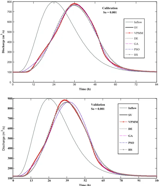
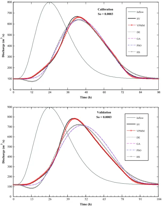
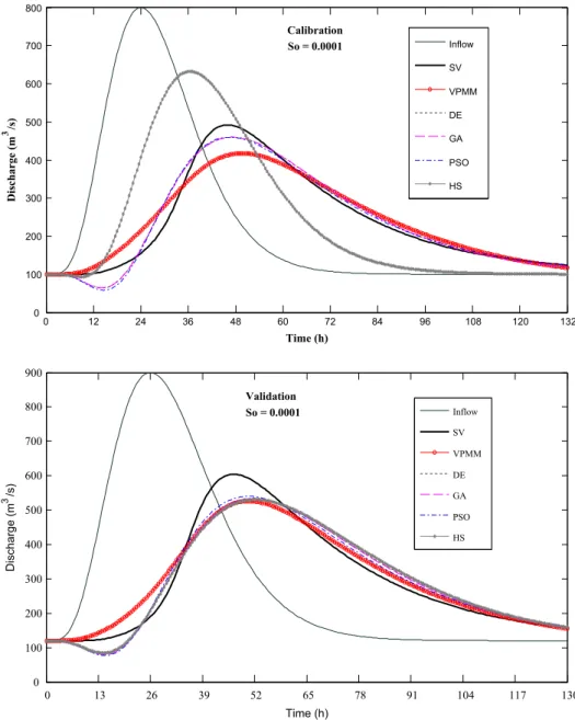
6. Results and discussion
Tables 2 and 3, respectively, show the comparative performance evaluations of the VPMM and AIA methods in reproducing the benchmark solutions corresponding to calibration and validation cases.Figs. 5–7, respectively, show the typical simulated discharge hydrographs of the VPMM and AIA methods for the calibration and validation cases of reproducing the respective benchmark solu-tions in channel reaches characterized by bed slopes So= 0.001,
0.0003 and 0.0001.
It is seen fromTables 2 and 3that the overall reproductions of the benchmark solutions by the VPMM method is more accurate
0 12 24 36 48 60 72 84 0 100 200 300 400 500 600 700 800 Time (h) Discharge (m 3 /s) Inflow SV VPMM DE GA PSO HS Calibration So = 0.001 0 13 26 39 52 65 78 91 104 100 200 300 400 500 600 700 800 900 Time (h) Discharge (m 3 /s) Inflow SV VPMM DE GA PSO HS Validation So = 0.001
than the corresponding reproductions by all the AIA methods stud-ied in the calibration cases, but much more accurate in the valida-tion cases, except for the case of routing in channel type-10 which is characterized by a very small slope ofSo= 0.0001. The water
sur-face gradient (1/So) (@y/ox)maxestimated for the inflow hydrograph at the inlet section of this channel type-10 (So= 0.0001) routing is
0.6129 which is a case beyond the applicability limit of the VPMM method specified by the criterion (1/So) (@y/ox)max60.5 (Perumal and Price, 2013). This inference is also evident from the poor repro-duction of the peak discharge of the benchmark solution of the
considered small slope channel with an error of15.16% which
is larger than that of the corresponding error estimates of the AIA methods considered in the calibration case, except for the case of the HS method, which estimated a peak discharge error of 28.55%. It is seen fromTables 2 and 3that the VPMM is a fully mass conservative for the channel types considered for routing floods using both calibration and validation cases, as demonstrated by
Perumal and Price (2013)andPerumal et al. (2013).
It may be noted that all the AIA methods also conserve mass in calibration and validation cases of simulations, except for the case of simulations using GA method in the validation case. It is seen from these tables that the error in time to peak estimates of the simulated cases using the VPMM method ranges from 0.0 h to 1.5 h for the applicable cases and this inference is consistent for both the calibration and validation cases of simulations. However, the error in time to peak of all the simulations of the AIA methods ranges from6.0 h to 6.5 h, and these estimates are not consistent even for the simulations in calibration and validation cases of the same method.
Further, it can be inferred fromFigs. 5–7, andTables 2 and 3
that the VPMM method is able to reproduce the benchmark solu-tions very closely from the perspective of overall reproduction and peak reproduction of the benchmark hydrographs, both in cal-ibration and validation cases, except for the cases of routing in channel type-10 characterized by S0= 0.0001 and this case falls
beyond the applicability limit of the VPMM method (Perumal
0 12 24 36 48 60 72 84 96 0 100 200 300 400 500 600 700 800 Time (h) Discharge (m 3 /s) Inflow SV VPMM DE GA PSO HS Calibration So = 0.0003 0 13 26 39 52 65 78 91 104 0 100 200 300 400 500 600 700 800 900 Time (h) Discharge (m 3 /s) Inflow SV VPMM DE GA PSO HS Validation So = 0.0003
and Price, 2013); whereas, all the AIA methods are almost identical in reproducing the benchmark solutions except in the case of HS method which is inconsistent in reproducing the benchmark solu-tions. PSO method and, especially, the HS method often fall in local minimum while searching the solution space and thus resulting in poor performance in producing the hydrographs. Based on the above discussion of results it is inferred that the VPMM method is performing better than all the AIA methods studied herein both in the calibration and validation cases of simulations. Unlike the NLM method, the VPMM method also enables to estimate the stage hydrograph corresponding to the routed discharge hydrograph at the outlet of the routing reach similar to that of the hydraulic rout-ing method (Perumal and Price, 2013) which is a desirable feature of a routing method required for operational purposes such as flood forecasting and the design of flood protection structures. In view of this development, it is argued that the sustained use of storage equation as envisaged byGill (1978)to model the nonlin-ear characteristics of flood wave movement can no longer be justi-fied and the methods developed so far in this context be retired from the literature of the Muskingum method.
7. Conclusions
The study was undertaken with two objectives,viz., firstly, for the inter-comparison of the efficacy of the performances of the NLM method, which use some selected AIA techniques for param-eters estimation, from the perspective of overall and specific fea-tures reproduction of the benchmark hydrographs employed for calibration and verifications of the method, and secondly for inter-comparison of the performances of the NLM method and the VPMM method from the perspective of overall and specific
fea-tures reproductions of the same benchmark hydrographs
employed in the calibration and validation studies of the NLM method.
Based on the analysis of results of this study it is inferred that the use of a physically based variable parameter Muskingum rout-ing method, such as the VPMM method which is capable of accounting for nonlinear behavior of flood wave movement pro-cess without involving calibration propro-cess is more reliable, when applied within its applicability limits for routing applications, than the conceptual NLM method which performs very poorly in 0 12 24 36 48 60 72 84 96 108 120 132 0 100 200 300 400 500 600 700 800 Time (h) Discharge (m 3 /s) Inflow SV VPMM DE GA PSO HS Calibration So = 0.0001 0 13 26 39 52 65 78 91 104 117 130 0 100 200 300 400 500 600 700 800 900 Time (h) Discharge (m 3/s) Inflow SV VPMM DE GA PSO HS Validation So = 0.0001
reproducing the benchmark hydrographs in the validation case of the routing process.
It needs to be emphasized herein that the NLM method was envisaged byGill (1978)on the premises that the linear storage weighted discharge relationship of the classical Muskingum method is inadequate to model the nonlinear behavior of flood wave propagation in rivers and channels. While this proposition to extend the capability of the linear Muskingum method to cap-ture the nonlinear behavior of the flood wave propagation could be considered appropriate at that time when it was proposed, but the same viewpoint cannot be sustained any longer as the sta-ted deficiency of the linear Muskingum storage equation has been effectively overcome by various physically based methods devel-oped from 1978 which enabled the variation of the Muskingum parameters at every routing step using the relationships estab-lished with channel and flow characteristics by various theories. These theories resulted in significant improved understanding of the variable parameter Muskingum method which enables to extend the capability of the Muskingum method to model the non-linear behavior of flood wave movement by varying the parameters of the method at every routing time step, but retaining the form of the classical Muskingum routing equation. Especially the
develop-ment of the VPMM method (Perumal and Price, 2013), which
derives the storage equation of the classical Muskingum method from the momentum equation of the SV equations, justify he sus-tained use of the form of linear storage equation of the Muskingum method to model the nonlinear behavior of the flood wave move-ment without resorting to its modification in the form of nonlinear storage equation as envisaged byGill (1978). Therefore, the sus-tained use of storage equation as envisaged byGill (1978)to model the nonlinear characteristics of flood wave movement can no longer be justified and the methods developed so far in this context be retired from the literature of the Muskingum method.
Acknowledgements
The authors thankfully acknowledge the help rendered by Pro-fessor Roland K. Price, Emeritus ProPro-fessor, UNESCO-IHE, The Netherlands for sparing his code used in the routing study based on the solution of SVequations. All data used in the study is avail-able upon request from the corresponding author.
References
Apollov, B.A., Kalinin, G.P., Komarov, V.D., 1964. Hydrological Forecasting, Translated From Russian. Israel Program for Scientific Translation, Jerusalem.
Ayvaz, M.T., 2007. Simultaneous determination of aquifer parameters and zone structures with fuzzy c-means clustering and meta-heuristic harmony search algorithm. Adv. Water Resour. 30, 2326–2338.
Chau, K.W., 2007. A split-step particle swarm optimization algorithm in river stage forecasting. J. Hydrol. 34, 131–135.
Chow, V.T., Maidment, D.R., Mays, L.W., 1988. Applied Hydrology. McGraw-Hill, New York.
Clerc, M., Kennedy, J., 2002. The particle swarm-explosion, stability, and convergence in a multidimensional complex space. IEEE Trans. Evol. Comput. 6 (1), 58–73.
Cunge, J.A., 1969. On a subject of a flood propagation method (Muskingum method). J. Hydraul. Res. IAHR7 (2), 205–230.
Dooge, J.C.I., 1973. Linear theory of hydrologic systems, USDA, Agric. Res. Serv., Tech. Bull., No. 1468.
Dooge, J.C.I., Harley, B.H., 1967. Linear routing in uniform open channel. Int. Hydrol. Symp, Fort Collins, Colorado, USA 1, 57–63.
Dooge, J.C.I., Strupczewski, W.G., Napiorkowski, J.J., 1982. Hydrodynamic derivation of storage parameters of the Muskingum model. J. Hydrol. 54 (4), 371–387.
Fread, D.L., 1993. Flow routing. In: Maidment, D.R. (Ed.), Handbook of Hydrology. McGraw Hill, New York.
Geem, Z.W., Kim, J.H., Loganathan, G.V., 2001. A new heuristic optimization algorithm: harmony search. Simulation 76 (2), 60–68.
Geem, Z.W., 2006a. Parameter estimation for the nonlinear Muskingum model using the BFGS technique. J. Irrig. Drain. Eng., ASCE 132 (5), 474–478.
Geem, Z.W., 2006b. Optimal cost design of water distribution networks using harmony search. Eng. Optimiz. 38 (3), 259–280.
Gill, M.A., 1978. Flood Routing by the Muskingum method. J. Hydrol. 36, 353–363.
Goldberg, D.E., 1999. Genetic Algorithms. Addison-Wesley, USA.
Gurarslan, G., 2011. Identification of Groundwater Contaminant Source Locations and Release Histories by Using Differential Evolution Algorithm (In Turkish). Ph. D. Thesis. Pamukkale University, Denizli, Turkey.
Gurarslan, G., Karahan, H., 2011. Parameter Estimation Technique for the Nonlinear Muskingum Flood Routing Model. In: 6thEWRA International Symposium-Water Engineering and Management in a Changing Environment,Catania, Italy.
Karaboga, D., Okdem, S., 2004. A simple and global optimization algorithm for engineering problems: differential evolution algorithm. Turk. J. Elect. Eng. 12 (1), 53–60.
Karahan, H., 2011. Obtaining Regional Rainfall-Intensity-Duration-Frequency Relationship Curves by Using Differential Evolution Algorithm. Scientific Research Project of TUBITAK (108Y299), Denizli, Turkey (In Turkish).
Karahan, H., 2012. Determining rainfall-intensity-duration-frequency relationship using Particle Swarm Optimization. KSCE J. Civil Eng. 16 (4), 667–675.
Karahan, H., Gurarslan, G., Geem, Z.W., 2013. Parameter estimation of the nonlinear Muskingum flood routing model using a hybrid harmony search algorithm. J. Hydrol. Eng. 18 (3), 352–360.
Kayhan, A.H., Ceylan, H., Ayvaz, M.T., Gurarslan, G., 2010. PSOLVER: A new hybrid particle swarm optimization algorithm for solving continuous optimization problems. Expert Syst. Appl. 37 (10), 6798–6808.
Kim, J.H., Geem, Z.W., Kim, E.S., 2001. Parameter estimation of the nonlinear Muskingum model using harmony search. J. Am. Water Resour. Assoc. 37 (5), 1131–1138.
Koussis, A.D., 1976. An approximate dynamic flood routing method, Proc. Int. Symp. On unsteady Flow in Open Channels, Paper L1, Newcastle-Upon Tyne, U.K.
Kumar, D.N., Reddy, M.J., 2007. Multipurpose reservoir operation using particle swarm optimization. J. Water Resour. Plan. Manage. ASCE 133 (3), 192–201.
Kundzewicz, Z.W., 1986. Physically based hydrologic flood routing method. Hydrol. Sci. J., IAHS 31 (2), 237–261.
Liong, S.Y., Chan, W.T., ShreeRam, J., 1995. Peak flow forecasting with genetic algorithm and SWMM. J. Hydraul. Eng. 121 (8), 613–617.
McCarthy, G.T., 1938. The unit hydrograph and flood routing. In: Conference of North Atlantic Div., U.S. Army Corps of Engineers.
Mohan, S., 1997. Parameter estimation of nonlinear Muskingum models using genetic algorithm. J. Hydraul. Eng., ASCE 123 (2), 137–142.
Perumal, M., 1992. The cause of negative initial outflow with the Muskingum method. Hydrol. Sci. J. 37 (4), 391–4401.
Perumal, M., 1994. Hydrodynamic derivation of a variable parameter Muskingum method-Part 1: Theory and solution procedure. Hydrol. Sci. J. IASH 39 (5), 431– 442.
Perumal, M., Sahoo, B., 2008. Volume conservation controversy of the variable parameter Muskingum-Cunge method. J. Hydraul. Eng., ASCE 134 (4), 475–485.
Perumal, M., Price, R.K., 2013. A fully volume conservative variable parameter McCarthy-Muskingum method: theory and Verification. J. Hydrol. 502, 89–102. Perumal, M., Naren, A., Ch. Madhusudana, R., 2013. Appraisal of two forms of non-linear Muskingum flood routing methods.6th International Perspective on Water Resources & the Environment. January 7–9, Izmir, Turkey, Proceeding paper number: IPWE2013-304.
Ponce, V.M., Yevjevich, V., 1978. Muskingum-Cunge method with variable parameters. J.Hydraul. Div., ASCE 104 (HY12), 1663–1667.
Ponce, V.M., Chaganti, P.V., 1994. Variable parameter Muskingum-Cunge method revisited. J. Hydrol. 162 (3–4), 433–439.
Price, R.K., 2009. Volume conservative, nonlinear routing. J. Hydraul. Eng., ASCE 135 (10), 838–845.http://dx.doi.org/10.1061/(ASCE)HY.1943-7900.0000088.
Saint-Venant, A.J.C., 1871a. Théorie du Mouvement Non Permanent des Eaux, avec Application aux Crues de Rivières et à l’Introduction des Marées dans leur Lit. Comptes Rendus des séances de l’Académie des Sciences, Paris, France 73 (4), 237–240 (in French).
Saint-Venant, A.J.C., 1871b. Théorie et Equations Générales du Mouvement Non Permanent des Eaux Courantes, Comptes Rendus des séances de l’Académie des Sciences, Paris, France, Séance, 73(17 July), 147–154 (in French).
Storn, R., Price, K., 1997. Differential evolution-a simple and efficient heuristic for global optimization over continuous spaces. J. Global Optim. 11, 341–359.
Strupczewski, W.G., Kundzewicz, Z.W., 1980. Muskingum method revisited. J. Hydrol. 48, 327–342.
Sen, Z., 2004. Genetic algorithm and optimization methods. Su VakfiYayinlari, Istanbul (Turkish). ISBN: 975-6455-12-8.
Shi, Y., Eberhart, R., 1998. A modified particle swarm optimizer. In: Proceedings of the IEEE International Conference on Evolutionary Computation, Anchorage, Alaska, pp. 69–73.
Tayfur, G., 2012. Soft Computing Methods in Water Resources Engineering. WIT Press, Southampton, England. 267 p..
Todini, E., 2007. A mass conservative and water storage consistent variable parameter Muskingum-Cunge approach. Hydrol. Earth Syst. Sci. 11, 1645–1659.
Tung, Y.K., 1985. Flood routing by nonlinear Muskingum method. J. Hydrol., ASCE 111 (12), 1447–1460.
Vasan, A., Simonovic, S., 2010. Optimization of water distribution network design using differential evolution. J. Water Plan. Manage. 136 (2), 279–287.
Yoon, J., Padmanabhan, G., 1993. Estimation of linear and nonlinear Muskingum models. J. Water Resource Manage. ASCE 19 (5), 600–610.